Tài liệu Fundamentals of Financial Management (2003) Chapter 6-11 doc

SOURCE: Beard, William Holbrook (1823–1900). New York Historical Society/The Bridgeman Art Library
International, Ltd.
CHAPTER
Risk and Rates
of Return
6
30
around, you’re not tied to the fickleness of a given
market, stock, or industry. . . . Correlation, in
portfolio-manager speak, helps you diversify properly
because it describes how closely two investments track
each other. If they move in tandem, they’re likely to
suffer from the same bad news. So, you should combine
assets with low correlations.”
U.S. investors tend to think of “the stock market” as
the U.S. stock market. However, U.S. stocks amount to
only 35 percent of the value of all stocks. Foreign
markets have been quite profitable, and they are not
perfectly correlated with U.S. markets. Therefore, global
diversification offers U.S. investors an opportunity to
raise returns and at the same time reduce risk. However,
foreign investing brings some risks of its own, most
notably “exchange rate risk,” which is the danger that
exchange rate shifts will decrease the number of dollars
a foreign currency will buy.
Although the central thrust of the Business Week
article was on ways to measure and then reduce risk, it
did point out that some recently created instruments
that are actually extremely risky have been marketed as
low-risk investments to naive investors. For example,

several mutual funds have advertised that their
portfolios “contain only securities backed by the U.S.
government” but then failed to highlight that the funds
themselves are using financial leverage, are investing in
f someone had invested $1,000 in a portfolio of
large-company stocks in 1925 and then reinvested
all dividends received, his or her investment would
have grown to $2,845,697 by 1999. Over the same
time period, a portfolio of small-company stocks would
have grown even more, to $6,641,505. But if instead he
or she had invested in long-term government bonds, the
$1,000 would have grown to only $40,219, and to a
measly $15,642 for short-term bonds.
Given these numbers, why would anyone invest in
bonds? The answer is, “Because bonds are less risky.”
While common stocks have over the past 74 years
produced considerably higher returns, (1) we cannot be
sure that the past is a prologue to the future, and (2)
stock values are more likely to experience sharp declines
than bonds, so one has a greater chance of losing
money on a stock investment. For example, in 1990 the
average small-company stock lost 21.6 percent of its
value, and large-company stocks also suffered losses.
Bonds, though, provided positive returns that year, as
they almost always do.
Of course, some stocks are riskier than others, and
even in years when the overall stock market goes up,
many individual stocks go down. Therefore, putting all
your money into one stock is extremely risky. According
to a Business Week article, the single best weapon

against risk is diversification: “By spreading your money
NO PAIN
NO GAIN
$
I
231
CHAPTER 6 ■ RISK AND RATES OF RETURN
232
In this chapter, we start from the basic premise that investors like returns and dis-
like risk. Therefore, people will invest in risky assets only if they expect to receive
higher returns. We define precisely what the term risk means as it relates to in-
vestments, we examine procedures managers use to measure risk, and we discuss
the relationship between risk and return. Then, in Chapters 7, 8, and 9, we extend
these relationships to show how risk and return interact to determine security
prices. Managers must understand these concepts and think about them as they
plan the actions that will shape their firms’ futures.
As you will see, risk can be measured in different ways, and different conclu-
sions about an asset’s riskiness can be reached depending on the measure used.
Risk analysis can be confusing, but it will help if you remember the following:
1. All financial assets are expected to produce cash flows, and the riskiness of
an asset is judged in terms of the riskiness of its cash flows.
2. The riskiness of an asset can be considered in two ways: (1) on a stand-
alone basis, where the asset’s cash flows are analyzed by themselves, or (2) in
a portfolio context, where the cash flows from a number of assets are com-
bined, and then the consolidated cash flows are analyzed.
1
There is an im-
portant difference between stand-alone and portfolio risk, and an asset that
has a great deal of risk if held by itself may be much less risky if it is held
as part of a larger portfolio.

3. In a portfolio context, an asset’s risk can be divided into two components:
(a) diversifiable risk, which can be diversified away and thus is of little con-
1
A portfolio is a collection of investment securities. If you owned some General Motors stock, some
Exxon Mobil stock, and some IBM stock, you would be holding a three-stock portfolio. Because di-
versification lowers risk, most stocks are held in portfolios.
SOURCES: “Figuring Risk: It’s Not So Scary,” Business Week,
November 1, 1993, 154–155; “T-Bill Trauma and the Meaning of
Risk,” The Wall Street Journal, February 12, 1993, C1; and
Stocks, Bonds, Bills, and Inflation: (Valuation Edition) 2000
Yearbook (Chicago: Ibbotson Associates, 2000).
“derivatives,” or are taking some other action that
boosts current yields but exposes investors to huge
risks.
When you finish this chapter, you should understand
what risk is, how it is measured, and what actions can
be taken to minimize it, or at least to ensure that you
are adequately compensated for bearing it. ■
233
cern to diversified investors, and (b) market risk, which reflects the risk of
a general stock market decline and which cannot be eliminated by diversifi-
cation, hence does concern investors. Only market risk is relevant — diver-
sifiable risk is irrelevant to rational investors because it can be eliminated.
4. An asset with a high degree of relevant (market) risk must provide a rela-
tively high expected rate of return to attract investors. Investors in general
are averse to risk, so they will not buy risky assets unless those assets have
high expected returns.
5. In this chapter, we focus on financial assets such as stocks and bonds, but
the concepts discussed here also apply to physical assets such as computers,
trucks, or even whole plants. ■

INVESTMENT RETURNS
With most investments, an individual or business spends money today with the
expectation of earning even more money in the future. The concept of return
provides investors with a convenient way of expressing the financial perfor-
mance of an investment. To illustrate, suppose you buy 10 shares of a stock for
$1,000. The stock pays no dividends, but at the end of one year, you sell the
stock for $1,100. What is the return on your $1,000 investment?
One way of expressing an investment return is in dollar terms. The dollar return
is simply the total dollars received from the investment less the amount invested:
Dollar return ϭ Amount received Ϫ Amount invested
ϭ $1,100 Ϫ $1,000
ϭ $100.
If at the end of the year you had sold the stock for only $900, your dollar re-
turn would have been Ϫ$100.
Although expressing returns in dollars is easy, two problems arise: (1) To
make a meaningful judgment about the return, you need to know the scale
(size) of the investment; a $100 return on a $100 investment is a good return
(assuming the investment is held for one year), but a $100 return on a $10,000
investment would be a poor return. (2) You also need to know the timing of the
return; a $100 return on a $100 investment is a very good return if it occurs
after one year, but the same dollar return after 20 years would not be very good.
The solution to the scale and timing problems is to express investment results
as rates of return, or percentage returns. For example, the rate of return on the
1-year stock investment, when $1,100 is received after one year, is 10 percent:
The rate of return calculation “standardizes” the return by considering the re-
turn per unit of investment. In this example, the return of 0.10, or 10 percent,
indicates that each dollar invested will earn 0.10($1.00) ϭ $0.10. If the rate of
ϭ 0.10 ϭ 10%.
ϭ
Dollar return

Amount invested
ϭ
$100
$1,000
Rate of return ϭ
Amount received Ϫ Amount invested
Amount invested
INVESTMENT RETURNS
CHAPTER 6 ■ RISK AND RATES OF RETURN
234
return had been negative, this would indicate that the original investment was
not even recovered. For example, selling the stock for only $900 results in a
Ϫ10 percent rate of return, which means that each dollar invested lost 10 cents.
Note also that a $10 return on a $100 investment produces a 10 percent rate of
return, while a $10 return on a $1,000 investment results in a rate of return of only
1 percent. Thus, the percentage return takes account of the size of the investment.
Expressing rates of return on an annual basis, which is typically done in
practice, solves the timing problem. A $10 return after one year on a $100 in-
vestment results in a 10 percent annual rate of return, while a $10 return after
five years yields only a 1.9 percent annual rate of return. We will discuss all this
in detail in Chapter 7, which deals with the time value of money.
Although we illustrated return concepts with one outflow and one inflow, in
later chapters we demonstrate that rate of return concepts can easily be applied
in situations where multiple cash flows occur over time. For example, when
Intel makes an investment in new chip-making technology, the investment is
made over several years and the resulting inflows occur over even more years.
For now, it is sufficient to recognize that the rate of return solves the two major
problems associated with dollar returns, size and timing. Therefore, the rate of
return is the most common measure of investment performance.
SELF-TEST QUESTIONS

Differentiate between dollar return and rate of return.
Why is the rate of return superior to the dollar return in terms of account-
ing for the size of investment and the timing of cash flows?
STAND-ALONE RISK
Risk is defined in Webster’s as “a hazard; a peril; exposure to loss or injury.”
Thus, risk refers to the chance that some unfavorable event will occur. If you
engage in skydiving, you are taking a chance with your life — skydiving is risky.
If you bet on the horses, you are risking your money. If you invest in specula-
tive stocks (or, really, any stock), you are taking a risk in the hope of making an
appreciable return.
An asset’s risk can be analyzed in two ways: (1) on a stand-alone basis, where
the asset is considered in isolation, and (2) on a portfolio basis, where the asset
is held as one of a number of assets in a portfolio. Thus, an asset’s stand-alone
risk is the risk an investor would face if he or she held only this one asset. Ob-
viously, most assets are held in portfolios, but it is necessary to understand
stand-alone risk in order to understand risk in a portfolio context.
To illustrate the riskiness of financial assets, suppose an investor buys
$100,000 of short-term Treasury bills with an expected return of 5 percent. In
this case, the rate of return on the investment, 5 percent, can be estimated quite
precisely, and the investment is defined as being essentially risk free. However,
if the $100,000 were invested in the stock of a company just being organized to
prospect for oil in the mid-Atlantic, then the investment’s return could not be
Risk
The chance that some unfavorable
event will occur.
Stand-Alone Risk
The risk an investor would face if
he or she held only one asset.
235
estimated precisely. One might analyze the situation and conclude that the ex-

pected rate of return, in a statistical sense, is 20 percent, but the investor should
also recognize that the actual rate of return could range from, say, ϩ1,000 per-
cent to Ϫ100 percent. Because there is a significant danger of actually earning
much less than the expected return, the stock would be relatively risky.
No investment will be undertaken unless the expected rate of return is high enough
to compensate the investor for the perceived risk of the investment. In our example, it
is clear that few if any investors would be willing to buy the oil company’s stock
if its expected return were the same as that of the T-bill.
Risky assets rarely produce their expected rates of return — generally, risky
assets earn either more or less than was originally expected. Indeed, if assets al-
ways produced their expected returns, they would not be risky. Investment risk,
then, is related to the probability of actually earning a low or negative return —
the greater the chance of a low or negative return, the riskier the investment.
However, risk can be defined more precisely, and we do so in the next section.
PROBABILITY DISTRIBUTIONS
An event’s probability is defined as the chance that the event will occur. For ex-
ample, a weather forecaster might state, “There is a 40 percent chance of rain
today and a 60 percent chance that it will not rain.” If all possible events, or
outcomes, are listed, and if a probability is assigned to each event, the listing is
called a probability distribution. For our weather forecast, we could set up the
following probability distribution:
OUTCOME PROBABILITY
(1) (2)
Rain 0.4 ϭ 40%
No rain 0.6 ϭ 60%
1.0 ϭ 100%
The possible outcomes are listed in Column 1, while the probabilities of these
outcomes, expressed both as decimals and as percentages, are given in Col-
umn 2. Notice that the probabilities must sum to 1.0, or 100 percent.
Probabilities can also be assigned to the possible outcomes (or returns) from

an investment. If you buy a bond, you expect to receive interest on the bond
plus a return of your original investment, and those payments will provide you
with a rate of return on your investment. The possible outcomes from this in-
vestment are (1) that the issuer will make the required payments or (2) that the
issuer will default on the payments. The higher the probability of default, the
riskier the bond, and the higher the risk, the higher the required rate of return.
If you invest in a stock instead of buying a bond, you will again expect to earn
a return on your money. A stock’s return will come from dividends plus capital
gains. Again, the riskier the stock — which means the higher the probability
that the firm will fail to perform as you expected — the higher the expected re-
turn must be to induce you to invest in the stock.
With this in mind, consider the possible rates of return (dividend yield plus
capital gain or loss) that you might earn next year on a $10,000 investment in
the stock of either Martin Products Inc. or U.S. Water Company. Martin man-
STAND-ALONE RISK
Probability Distribution
A listing of all possible outcomes,
or events, with a probability
(chance of occurrence) assigned to
each outcome.
CHAPTER 6 ■ RISK AND RATES OF RETURN
236
ufactures and distributes computer terminals and equipment for the rapidly
growing data transmission industry. Because it faces intense competition, its
new products may or may not be competitive in the marketplace, so its future
earnings cannot be predicted very well. Indeed, some new company could de-
velop better products and literally bankrupt Martin. U.S. Water, on the other
hand, supplies an essential service, and because it has city franchises that pro-
tect it from competition, its sales and profits are relatively stable and pre-
dictable.

The rate-of-return probability distributions for the two companies are
shown in Table 6-1. There is a 30 percent chance of strong demand, in which
case both companies will have high earnings, pay high dividends, and enjoy
capital gains. There is a 40 percent probability of normal demand and moder-
ate returns, and there is a 30 percent probability of weak demand, which will
mean low earnings and dividends as well as capital losses. Notice, however, that
Martin Products’ rate of return could vary far more widely than that of U.S.
Water. There is a fairly high probability that the value of Martin’s stock will
drop substantially, resulting in a 70 percent loss, while there is no chance of a
loss for U.S. Water.
2
E
XPECTED RATE OF
RETURN
If we multiply each possible outcome by its probability of occurrence and then
sum these products, as in Table 6-2, we have a weighted average of outcomes.
The weights are the probabilities, and the weighted average is the expected
rate of return, k
ˆ
, called “k-hat.”
3
The expected rates of return for both Mar-
tin Products and U.S. Water are shown in Table 6-2 to be 15 percent. This type
of table is known as a payoff matrix.
TABLE 6-1
RATE OF RETURN ON STOCK
IF THIS DEMAND OCCURS
DEMAND FOR THE PROBABILITY OF THIS
COMPANY’S PRODUCTS DEMAND OCCURRING MARTIN PRODUCTS U.S. WATER
Strong 0.3 100% 20%

Normal 0.4 15 15
Weak 0.3 (70) 10
1.0
Probability Distributions for Martin Products and U.S. Water
2
It is, of course, completely unrealistic to think that any stock has no chance of a loss. Only in hy-
pothetical examples could this occur. To illustrate, the price of Columbia Gas’s stock dropped from
$34.50 to $20.00 in just three hours a few years ago. All investors were reminded that any stock is
exposed to some risk of loss, and those investors who bought Columbia Gas learned that lesson the
hard way.
3
In Chapters 8 and 9, we will use k
d
and k
s
to signify the returns on bonds and stocks, respectively.
However, this distinction is unnecessary in this chapter, so we just use the general term, k, to sig-
nify the expected return on an investment.
Expected Rate of Return, k
ˆ
The rate of return expected to be
realized from an investment; the
weighted average of the
probability distribution of possible
results.
237
The expected rate of return calculation can also be expressed as an equation
that does the same thing as the payoff matrix table:
4
Expected rate of return ϭ k

ˆ
ϭ P
1
k
1
ϩ P
2
k
2
ϩиииϩP
n
k
n
. (6-1)
Here k
i
is the ith possible outcome, P
i
is the probability of the ith outcome, and
n is the number of possible outcomes. Thus, k
ˆ
is a weighted average of the pos-
sible outcomes (the k
i
values), with each outcome’s weight being its probability
of occurrence. Using the data for Martin Products, we obtain its expected rate
of return as follows:
k
ˆ
ϭ P

1
(k
1
) ϩ P
2
(k
2
) ϩ P
3
(k
3
)
ϭ 0.3(100%) ϩ 0.4(15%) ϩ 0.3(Ϫ70%)
ϭ 15%.
U.S. Water’s expected rate of return is also 15 percent:
k
ˆ
ϭ 0.3(20%) ϩ 0.4(15%) ϩ 0.3(10%)
ϭ 15%.
We can graph the rates of return to obtain a picture of the variability of pos-
sible outcomes; this is shown in the Figure 6-1 bar charts. The height of each
bar signifies the probability that a given outcome will occur. The range of
probable returns for Martin Products is from Ϫ70 to ϩ100 percent, with an ex-
pected return of 15 percent. The expected return for U.S. Water is also 15 per-
cent, but its range is much narrower.
Thus far, we have assumed that only three situations can exist: strong, nor-
mal, and weak demand. Actually, of course, demand could range from a deep de-
pression to a fantastic boom, and there are an unlimited number of possibilities
ϭ
a

n
iϭ1
P
i
k
i
STAND-ALONE RISK
TABLE 6-2
MARTIN PRODUCTS U.S. WATER
DEMAND FOR PROBABILITY RATE OF RETURN RATE OF RETURN
THE COMPANY’S OF THIS DEMAND IF THIS DEMAND PRODUCT: IF THIS DEMAND PRODUCT:
PRODUCTS OCCURRING OCCURS (2) ؋ (3) OCCURS (2) ؋ (5)
(1) (2) (3) ؍ (4) (5) ؍ (6)
Strong 0.3 100% 30% 20% 6%
Normal 0.4 15 6 15 6
Weak 0.3 (70) (21)1 10 13%
1.0 k
ˆ
ϭ 15% k
ˆ
ϭ 15%
Calculation of Expected Rates of Return: Payoff Matrix
4
The second form of the equation is simply a shorthand expression in which sigma (⌺) means
“sum up,” or add the values of n factors. If i ϭ 1, then P
i
k
i
ϭ P
1

k
1
;ifiϭ 2, then P
i
k
i
ϭ P
2
k
2
; and so
on until i ϭ n, the last possible outcome. The symbol simply says, “Go through the following
process: First, let i ϭ 1 and find the first product; then let i ϭ 2 and find the second product; then
continue until each individual product up to i ϭ n has been found, and then add these individual
products to find the expected rate of return.”
a
n
iϭ1
CHAPTER 6 ■ RISK AND RATES OF RETURN
238
in between. Suppose we had the time and patience to assign a probability to
each possible level of demand (with the sum of the probabilities still equaling
1.0) and to assign a rate of return to each stock for each level of demand. We
would have a table similar to Table 6-1, except that it would have many more
entries in each column. This table could be used to calculate expected rates of
return as shown previously, and the probabilities and outcomes could be ap-
proximated by continuous curves such as those presented in Figure 6-2. Here
we have changed the assumptions so that there is essentially a zero probability
that Martin Products’ return will be less than Ϫ70 percent or more than 100
percent, or that U.S. Water’s return will be less than 10 percent or more than

20 percent, but virtually any return within these limits is possible.
The tighter, or more peaked, the probability distribution, the more likely it is that
the actual outcome will be close to the expected value, and, consequently, the less likely
it is that the actual return will end up far below the expected return. Thus, the tighter
the probability distribution, the lower the risk assigned to a stock. Since U.S. Water
has a relatively tight probability distribution, its actual return is likely to be
closer to its 15 percent expected return than is that of Martin Products.
MEASURING STAND-ALONE RISK:
T
HE STANDARD DEVIATION
Risk is a difficult concept to grasp, and a great deal of controversy has sur-
rounded attempts to define and measure it. However, a common definition, and
one that is satisfactory for many purposes, is stated in terms of probability distri-
FIGURE 6-1
Probability Distributions of Martin Products’
and U.S. Water’s Rates of Return
Probability of
Occurrence
a. Martin Products
Rate of Return
(%)
100150–70
0.4
0.3
0.2
0.1
Expected Rate
of Return
Probability of
Occurrence

b. U.S. Water
Rate of Return
(%)
2015010
0.4
0.3
0.2
0.1
Expected Rate
of Return
239
butions such as those presented in Figure 6-2: The tighter the probability distribu-
tion of expected future returns, the smaller the risk of a given investment. According to
this definition, U.S. Water is less risky than Martin Products because there is a
smaller chance that its actual return will end up far below its expected return.
To be most useful, any measure of risk should have a definite value — we
need a measure of the tightness of the probability distribution. One such mea-
sure is the standard deviation, the symbol for which is ␴, pronounced “sigma.”
The smaller the standard deviation, the tighter the probability distribution,
and, accordingly, the lower the riskiness of the stock. To calculate the standard
deviation, we proceed as shown in Table 6-3, taking the following steps:
1. Calculate the expected rate of return:
For Martin, we previously found k
ˆ
ϭ 15%.
2. Subtract the expected rate of return (k
ˆ
) from each possible outcome (k
i
)

to obtain a set of deviations about k
ˆ
as shown in Column 1 of Table 6-3:
Deviation
i
ϭ k
i
Ϫ k
ˆ
.
Expected rate of return ϭ
ˆ
k ϭ
a
n
iϭ1
P
i
k
i
.
STAND-ALONE RISK
FIGURE 6-2
Continuous Probability Distributions of Martin Products’
and U.S. Water’s Rates of Return
Probability Density
U.S. Water
Martin Products
100150–70
Expected

Rate of Return
Rate of Return
(%)
NOTE: The assumptions regarding the probabilities of various outcomes have been changed from those
in Figure 6-1. There the probability of obtaining exactly 15 percent was 40 percent; here it is much
smaller because there are many possible outcomes instead of just three. With continuous distributions,
it is more appropriate to ask what the probability is of obtaining at least some specified rate of return
than to ask what the probability is of obtaining exactly that rate. This topic is covered in detail in
statistics courses.
Standard Deviation, ␴
A statistical measure of the
variability of a set of observations.
CHAPTER 6 ■ RISK AND RATES OF RETURN
240
3. Square each deviation, then multiply the result by the probability of oc-
currence for its related outcome, and then sum these products to obtain
the variance of the probability distribution as shown in Columns 2 and 3
of the table:
(6-2)
4. Finally, find the square root of the variance to obtain the standard devia-
tion:
(6-3)
Thus, the standard deviation is essentially a weighted average of the deviations
from the expected value, and it provides an idea of how far above or below the
expected value the actual value is likely to be. Martin’s standard deviation is
seen in Table 6-3 to be ␴ ϭ 65.84%. Using these same procedures, we find
U.S. Water’s standard deviation to be 3.87 percent. Martin Products has the
larger standard deviation, which indicates a greater variation of returns and
thus a greater chance that the expected return will not be realized. Therefore,
Martin Products is a riskier investment than U.S. Water when held alone.

If a probability distribution is normal, the actual return will be within Ϯ1
standard deviation of the expected return 68.26 percent of the time. Figure 6-3
illustrates this point, and it also shows the situation for Ϯ2␴ and Ϯ3␴. For
Martin Products, k
ˆ
ϭ 15% and ␴ ϭ 65.84%, whereas k
ˆ
ϭ 15% and ␴ ϭ 3.87%
for U.S. Water. Thus, if the two distributions were normal, there would be a
68.26 percent probability that Martin’s actual return would be in the range of
15 Ϯ 65.84 percent, or from Ϫ50.84 to 80.84 percent. For U.S. Water, the
68.26 percent range is 15 Ϯ 3.87 percent, or from 11.13 to 18.87 percent. With
such a small ␴, there is only a small probability that U.S. Water’s return would
be significantly less than expected, so the stock is not very risky. For the aver-
age firm listed on the New York Stock Exchange, ␴ has generally been in the
range of 35 to 40 percent in recent years.
5
Standard deviation ϭ ␴ ϭ
B
a
n
iϭ1
(k
i
Ϫ
ˆ
k)
2
P
i

.
Variance ϭ ␴
2
ϭ
a
n
iϭ1
(k
i
Ϫ
ˆ
k)
2
P
i
.
TABLE 6-3
k
i
؊ k
ˆ
(k
i
؊ k
ˆ
)
2
(k
i
؊ k

ˆ
)
2
P
i
(1) (2) (3)
100 Ϫ 15 ϭ 85 7,225 (7,225)(0.3) ϭ 2,167.5
15 Ϫ 15 ϭ 0 0 (0)(0.4) ϭ 0.0
Ϫ70 Ϫ 15 ϭϪ85 7,225 (7,225)(0.3) ϭ 2,167.5
Variance ϭ ␴
2
ϭ 4,335.0
Standard deviation ϭ ␴ ϭ ͙␴
ෆ
2
ෆ
ϭ ͙4
ෆ
,3
ෆ
3
ෆ
5
ෆ
ϭ 65.84%.
Calculating Martin Products’ Standard Deviation
Variance, ␴
2
The square of the standard
deviation.

Wilshire Associates
provides a download site
for various returns series
for indexes such as the
Wilshire 5000 and the
Wilshire 4500 at http://
www.wilshire.com/indexes/wilshire_
indexes.htm in Microsoft Excel
TM
format.
5
In the example, we described the procedure for finding the mean and standard deviation when the
data are in the form of a known probability distribution. If only sample returns data over some past
period are available, the standard deviation of returns can be estimated using this formula:
(footnote continues)
241
STAND-ALONE RISK
FIGURE 6-3
Probability Ranges for a Normal Distribution
+3σ+2σ+1σ–1σ k–2σ–3σ
ˆ
68.26%
95.46%
99.74%
NOTES:
a. The area under the normal curve always equals 1.0, or 100 percent. Thus, the areas under any pair of
normal curves drawn on the same scale, whether they are peaked or flat, must be equal.
b. Half of the area under a normal curve is to the left of the mean, indicating that there is a 50
percent probability that the actual outcome will be less than the mean, and half is to the right of
k, indicating a 50 percent probability that it will be greater than the mean.

c. Of the area under the curve, 68.26 percent is within Ϯ1␴ of the mean, indicating that the
probability is 68.26 percent that the actual outcome will be within the range k Ϫ 1␴ to k ϩ 1␴.
d. Procedures exist for finding the probability of other ranges. These procedures are covered in
statistics courses.
e. For a normal distribution, the larger the value of ␴, the greater the probability that the actual
outcome will vary widely from, and hence perhaps be far below, the expected, or most likely,
outcome. Since the probability of having the actual result turn out to be far below the expected result
is one definition of risk, and since ␴ measures this probability, we can use ␴ as a measure of risk.
This definition may not be a good one, however, if we are dealing with an asset held in a diversified
portfolio. This point is covered later in the chapter.
(6-3a)
Here k
ෆ
t
(“k bar t”) denotes the past realized rate of return in Period t, and k
ෆ
Avg
is the average an-
nual return earned during the last n years. Here is an example:
YEAR k
—
t
1999 15%
2000 Ϫ5
2001 20
ϭ
B
350
2
ϭ 13.2%.

Estimated ␴ (or S) ϭ
C
(15 Ϫ 10)
2
ϩ (Ϫ5 Ϫ 10)
2
ϩ (20 Ϫ 10)
2
3 Ϫ 1
k
Avg
ϭ
(15 Ϫ 5 ϩ 20)
3
ϭ 10.0%.
Estimated ␴ ϭ S ϭ
R
a
n
tϭ1
(k
t
Ϫ k
Avg
)
2
n Ϫ 1
.
(footnote continues)
(Footnote 5 continued)

CHAPTER 6 ■ RISK AND RATES OF RETURN
242
MEASURING STAND-ALONE RISK:
T
HE COEFFICIENT OF VARIATION
If a choice has to be made between two investments that have the same expected
returns but different standard deviations, most people would choose the one
with the lower standard deviation and, therefore, the lower risk. Similarly, given
a choice between two investments with the same risk (standard deviation) but
different expected returns, investors would generally prefer the investment with
the higher expected return. To most people, this is common sense — return is
“good,” risk is “bad,” and, consequently, investors want as much return and as
little risk as possible. But how do we choose between two investments if one has
the higher expected return but the other the lower standard deviation? To help
answer this question, we use another measure of risk, the coefficient of varia-
tion (CV), which is the standard deviation divided by the expected return:
(6-4)
The coefficient of variation shows the risk per unit of return, and it provides a more
meaningful basis for comparison when the expected returns on two alternatives are not
the same. Since U.S. Water and Martin Products have the same expected return,
the coefficient of variation is not necessary in this case. The firm with the larger
standard deviation, Martin, must have the larger coefficient of variation when
the means are equal. In fact, the coefficient of variation for Martin is 65.84/15
ϭ 4.39 and that for U.S. Water is 3.87/15 ϭ 0.26. Thus, Martin is almost 17
times riskier than U.S. Water on the basis of this criterion.
For a case where the coefficient of variation is necessary, consider Projects X
and Y in Figure 6-4. These projects have different expected rates of return and
different standard deviations. Project X has a 60 percent expected rate of return
and a 15 percent standard deviation, while Project Y has an 8 percent expected
return but only a 3 percent standard deviation. Is Project X riskier, on a rela-

tive basis, because it has the larger standard deviation? If we calculate the coef-
ficients of variation for these two projects, we find that Project X has a coeffi-
cient of variation of 15/60 ϭ 0.25, and Project Y has a coefficient of variation
of 3/8 ϭ 0.375. Thus, we see that Project Y actually has more risk per unit of
return than Project X, in spite of the fact that X’s standard deviation is larger.
Therefore, even though Project Y has the lower standard deviation, according
to the coefficient of variation it is riskier than Project X.
Project Y has the smaller standard deviation, hence the more peaked proba-
bility distribution, but it is clear from the graph that the chances of a really low
Coefficient of variation ϭ CV ϭ
␴
ˆ
k
.
Coefficient of Variation (CV)
Standardized measure of the risk
per unit of return; calculated as
the standard deviation divided by
the expected return.
The historical ␴ is often used as an estimate of the future ␴. Much less often, and generally incor-
rectly, k
ෆ
Avg
for some past period is used as an estimate of k, the expected future return. Because past
variability is likely to be repeated, ␴ may be a good estimate of future risk, but it is much less rea-
sonable to expect that the past level of return (which could have been as high as ϩ100% or as low
as Ϫ50%) is the best expectation of what investors think will happen in the future.
Equation 6-3a is built into all financial calculators, and it is very easy to use. We simply enter
the rates of return and press the key marked S (or S
x

) to get the standard deviation. Note, though,
that calculators have no built-in formula for finding ␴ where probabilistic data are involved; there
you must go through the process outlined in Table 6-3 and Equation 6-3. The same situation holds
for computer spreadsheet programs.
(Footnote 5 continued)
243
return are higher for Y than for X because X’s expected return is so high. Be-
cause the coefficient of variation captures the effects of both risk and return, it
is a better measure for evaluating risk in situations where investments have sub-
stantially different expected returns.
RISK AVERSION AND REQUIRED RETURNS
Suppose you have worked hard and saved $1 million, which you now plan to in-
vest. You can buy a 5 percent U.S. Treasury note, and at the end of one year you
will have a sure $1.05 million, which is your original investment plus $50,000 in
interest. Alternatively, you can buy stock in R&D Enterprises. If R&D’s research
programs are successful, your stock will increase in value to $2.1 million. How-
ever, if the research is a failure, the value of your stock will go to zero, and you
will be penniless. You regard R&D’s chances of success or failure as being 50-50,
so the expected value of the stock investment is 0.5($0) ϩ 0.5($2,100,000) ϭ
$1,050,000. Subtracting the $1 million cost of the stock leaves an expected profit
of $50,000, or an expected (but risky) 5 percent rate of return:
Thus, you have a choice between a sure $50,000 profit (representing a 5 per-
cent rate of return) on the Treasury note and a risky expected $50,000 profit
(also representing a 5 percent expected rate of return) on the R&D Enterprises
stock. Which one would you choose? If you choose the less risky investment, you are
ϭ
$50,000
$1,000,000
ϭ 5%.
ϭ

$1,050,000 Ϫ $1,000,000
$1,000,000
Expected rate of return ϭ
Expected ending value Ϫ Cost
Cost
STAND-ALONE RISK
FIGURE 6-4
Comparison of Probability Distributions and Rates of Return
for Projects X and Y
08 60
Probability
Density
Project Y
Project X
Expected Rate
of Return (%)
THE TRADE-OFF BETWEEN RISK AND RETURN
CHAPTER 6 ■ RISK AND RATES OF RETURN
244
risk averse. Most investors are indeed risk averse, and certainly the average investor is
risk averse with regard to his or her “serious money.” Because this is a well-documented
fact, we shall assume risk aversion throughout the remainder of the book.
What are the implications of risk aversion for security prices and rates of re-
turn? The answer is that, other things held constant, the higher a security’s risk,
the lower its price and the higher its required return. To see how risk aversion af-
fects security prices, look back at Figure 6-2 and consider again U.S. Water and
T
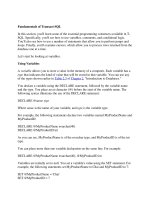
he table accompanying this box summarizes the historical
trade-off between risk and return for different classes of in-
vestments from 1926 through 1999. As the table shows, those

assets that produced the highest average returns also had the
highest standard deviations and the widest ranges of returns.
For example, small-company stocks had the highest average an-
nual return, 17.6 percent, but their standard deviation of re-
turns, 33.6 percent, was also the highest. By contrast, U.S.
Treasury bills had the lowest standard deviation, 3.2 percent,
but they also had the lowest average return, 3.8 percent.
When deciding among alternative investments, one needs to
be aware of the trade-off between risk and return. While there
is certainly no guarantee that history will repeat itself, returns
observed in the past are a good starting point for estimating
investments’ returns in the future. Likewise, the standard devi-
ations of past returns provide useful insights into the risks of
different investments. For T-bills, however, the standard devia-
tion needs to be interpreted carefully. Note that the table
shows that Treasury bills have a positive standard deviation,
which indicates some risk. However, if you invested in a one-
year Treasury bill and held it for the full year, your realized re-
turn would be the same regardless of what happened to the
economy that year, and thus the standard deviation of your re-
turn would be zero. So, why does the table show a 3.2 percent
standard deviation for T-bills, which indicates some risk? In
fact, a T-bill is riskless if you hold it for one year, but if you in-
vest in a rolling portfolio of one-year T-bills and hold the port-
folio for a number of years, your investment income will vary
depending on what happens to the level of interest rates in
each year. So, while you can be sure of the return you will earn
on a T-bill in a given year, you cannot be sure of the return you
will earn on a portfolio of T-bills over a period of time.
Risk Aversion

Risk-averse investors dislike risk
and require higher rates of return
as an inducement to buy riskier
securities.
Selected Realized Returns, 1926–1999
AVERAGE RETURN STANDARD DEVIATION
Small-company
stocks 17.6% 33.6%
Large-company
stocks 13.3 20.1
Long-term
corporate bonds 5.9 8.7
Long-term
goverment bonds 5.5 9.3
U.S. Treasury bills 3.8 3.2
Source: Based on Stocks, Bonds, Bills, and Inflation: (Valuation Edition) 2000 Yearbook (Chicago:
Ibbotson Associates, 2000), 14.
245
Martin Products stocks. Suppose each stock sold for $100 per share and each had
an expected rate of return of 15 percent. Investors are averse to risk, so under
these conditions there would be a general preference for U.S. Water. People
with money to invest would bid for U.S. Water rather than Martin stock, and
Martin’s stockholders would start selling their stock and using the money to buy
U.S. Water. Buying pressure would drive up U.S. Water’s stock, and selling pres-
sure would simultaneously cause Martin’s price to decline.
These price changes, in turn, would cause changes in the expected rates of re-
turn on the two securities. Suppose, for example, that U.S. Water’s stock price was
bid up from $100 to $150, whereas Martin’sstockpricedeclinedfrom$100to$75.
This would cause U.S. Water’s expected return to fall to 10 percent, while Mar-
tin’s expected return would rise to 20 percent. The difference in returns, 20% Ϫ

10% ϭ 10%,isarisk premium, RP, which represents the additional compensa-
tion investors require for assuming the additional risk of Martin stock.
This example demonstrates a very important principle: In a market dominated
by risk-averse investors, riskier securities must have higher expected returns, as esti-
mated by the marginal investor, than less risky securities. If this situation does not exist,
buying and selling in the market will force it to occur. We will consider the question
of how much higher the returns on risky securities must be later in the chapter,
after we see how diversification affects the way risk should be measured. Then,
in Chapters 8 and 9, we will see how risk-adjusted rates of return affect the
prices investors are willing to pay for different securities.
STAND-ALONE RISK
Risk Premium, RP
The difference between the
expected rate of return on a given
risky asset and that on a less risky
asset.
SELF-TEST QUESTIONS
What does “investment risk” mean?
Set up an illustrative probability distribution for an investment.
What is a payoff matrix?
Which of the two stocks graphed in Figure 6-2 is less risky? Why?
How does one calculate the standard deviation?
Which is a better measure of risk if assets have different expected returns:
(1) the standard deviation or (2) the coefficient of variation? Why?
Explain the following statement: “Most investors are risk averse.”
How does risk aversion affect rates of return?
RISK IN A PORTFOLIO CONTEXT
In the preceding section, we considered the riskiness of assets held in isolation.
Now we analyze the riskiness of assets held in portfolios. As we shall see, an
asset held as part of a portfolio is less risky than the same asset held in isolation.

Accordingly, most financial assets are held as parts of portfolios. Banks, pension
funds, insurance companies, mutual funds, and other financial institutions are
CHAPTER 6 ■ RISK AND RATES OF RETURN
246
required by law to hold diversified portfolios. Even individual investors — at
least those whose security holdings constitute a significant part of their total
wealth — generally hold portfolios, not the stock of only one firm. This being
the case, from an investor’s standpoint the fact that a particular stock goes up
or down is not very important; what is important is the return on his or her port-
folio, and the portfolio’s risk. Logically, then, the risk and return of an individual se-
curity should be analyzed in terms of how that security affects the risk and return of
the portfolio in which it is held.
To illustrate, Pay Up Inc. is a collection agency company that operates na-
tionwide through 37 offices. The company is not well known, its stock is not
very liquid, its earnings have fluctuated quite a bit in the past, and it doesn’t pay
a dividend. All this suggests that Pay Up is risky and that its required rate of re-
turn, k, should be relatively high. However, Pay Up’s required rate of return in
2001, and all other years, was quite low in comparison to those of most other
companies. This indicates that investors regard Pay Up as being a low-risk
company in spite of its uncertain profits. The reason for this counterintuitive
fact has to do with diversification and its effect on risk. Pay Up’s earnings rise
during recessions, whereas most other companies’ earnings tend to decline
when the economy slumps. It’s like fire insurance — it pays off when other
things go bad. Therefore, adding Pay Up to a portfolio of “normal” stocks
tends to stabilize returns on the entire portfolio, thus making the portfolio less
risky.
P
ORTFOLIO RETURNS
The expected return on a portfolio, k
ˆ

p
, is simply the weighted average of the
expected returns on the individual assets in the portfolio, with the weights
being the fraction of the total portfolio invested in each asset:
k
ˆ
p
ϭ w
1
k
ˆ
1
ϩ w
2
k
ˆ
2
ϩиииϩw
n
k
ˆ
n
(6-5)
Here the k
ˆ
i
’s are the expected returns on the individual stocks, the w
i
’s are the
weights, and there are n stocks in the portfolio. Note (1) that w

i
is the fraction
of the portfolio’s dollar value invested in Stock i (that is, the value of the in-
vestment in Stock i divided by the total value of the portfolio) and (2) that the
w
i
’s must sum to 1.0.
Assume that in August 2001, a security analyst estimated that the following
returns could be expected on the stocks of four large companies:
EXPECTED RETURN, k
ˆ
Microsoft 12.0%
General Electric 11.5
Pfizer 10.0
Coca-Cola 9.5
If we formed a $100,000 portfolio, investing $25,000 in each stock, the ex-
pected portfolio return would be 10.75%:
ϭ
a
n
iϭ1
w
i
ˆ
k
i
.
Expected Return on a
Portfolio,
ˆ

k
p
The weighted average of the
expected returns on the assets held
in the portfolio.
247
k
ˆ
p
ϭ w
1
k
ˆ
1
ϩ w
2
k
ˆ
2
ϩ w
3
k
ˆ
3
ϩ w
4
k
ˆ
4
ϭ 0.25(12%) ϩ 0.25(11.5%) ϩ 0.25(10%) ϩ 0.25(9.5%)

ϭ 10.75%.
Of course, after the fact and a year later, the actual realized rates of return, k
ෆ
,
on the individual stocks — the k
ෆ
i
, or “k-bar,” values — will almost certainly be
different from their expected values, so k
ෆ
p
will be different from k
ˆ
p
ϭ 10.75%.
For example, Coca-Cola stock might double in price and provide a return of
ϩ100%, whereas Microsoft stock might have a terrible year, fall sharply, and
have a return of Ϫ75%. Note, though, that those two events would be some-
what offsetting, so the portfolio’s return might still be close to its expected re-
turn, even though the individual stocks’ actual returns were far from their ex-
pected returns.
PORTFOLIO RISK
As we just saw, the expected return on a portfolio is simply the weighted aver-
age of the expected returns on the individual assets in the portfolio. However,
unlike returns, the riskiness of a portfolio, ␴
p
, is generally not the weighted
average of the standard deviations of the individual assets in the portfolio; the
portfolio’s risk will be smaller than the weighted average of the assets’ ␴’s. In
fact, it is theoretically possible to combine stocks that are individually quite

risky as measured by their standard deviations and to form a portfolio that is
completely riskless, with ␴
p
ϭ 0.
To illustrate the effect of combining assets, consider the situation in Figure
6-5. The bottom section gives data on rates of return for Stocks W and M in-
dividually, and also for a portfolio invested 50 percent in each stock. The three
top graphs show plots of the data in a time series format, and the lower graphs
show the probability distributions of returns, assuming that the future is ex-
pected to be like the past. The two stocks would be quite risky if they were held
in isolation, but when they are combined to form Portfolio WM, they are not
risky at all. (Note: These stocks are called W and M because the graphs of their
returns in Figure 6-5 resemble a W and an M.)
The reason Stocks W and M can be combined to form a riskless portfolio is
that their returns move countercyclically to each other — when W’s returns
fall, those of M rise, and vice versa. The tendency of two variables to move to-
gether is called correlation, and the correlation coefficient, r, measures this
tendency.
6
In statistical terms, we say that the returns on Stocks W and M are
perfectly negatively correlated, with r ϭϪ1.0.
The opposite of perfect negative correlation, with r ϭϪ1.0, is perfect positive
correlation, with r ϭϩ1.0. Returns on two perfectly positively correlated stocks
RISK IN A PORTFOLIO CONTEXT
Realized Rate of Return, k
ෆ
The return that was actually
earned during some past period.
The actual return (k
ෆ

) usually turns
out to be different from the
expected return (k
ˆ
) except for
riskless assets.
Correlation
The tendency of two variables to
move together.
Correlation Coefficient, r
A measure of the degree of
relationship between two
variables.
6
The correlation coefficient, r, can range from ϩ1.0, denoting that the two variables move up and
down in perfect synchronization, to Ϫ1.0, denoting that the variables always move in exactly op-
posite directions. A correlation coefficient of zero indicates that the two variables are not related to
each other — that is, changes in one variable are independent of changes in the other.
It is easy to calculate correlation coefficients with a financial calculator. Simply enter the returns
on the two stocks and then press a key labeled “r.” For W and M, r ϭϪ1.0.
CHAPTER 6 ■ RISK AND RATES OF RETURN
248
FIGURE 6-5
Rate of Return Distributions for Two Perfectly Negatively Correlated
Stocks (r ؍ ؊1.0) and for Portfolio WM
k (%)
W
_
a. Rates of Return
Stock W

2001
25
0
–10
15
k (%)
M
_
Stock M
2001
25
0
–10
15
k (%)
p
_
Portfolio WM
2001
25
0
–10
15
Percent150
(= k )
W
Probability
Density
Stock W
b. Probability Distributions of Returns

Percent150
Probability
Density
Stock M
Percent150
Probability
Density
Portfolio WM
(= k )
M
(= k )
p
ˆˆˆ
STOCK W STOCK M PORTFOLIO WM
YEAR (k
ෆ
W
)(k
ෆ
M
)(k
ෆ
p
)
1997 40.0% (10.0%) 15.0%
1998 (10.0) 40.0 15.0
1999 35.0 (5.0) 15.0
2000 (5.0) 35.0 15.0
2001 15.0% 15.0% 15.0%
Average return 15.0% 15.0% 15.0%

Standard deviation 22.6% 22.6% 0.0%
249
(M and MЈ) would move up and down together, and a portfolio consisting of
two such stocks would be exactly as risky as the individual stocks. This point is
illustrated in Figure 6-6, where we see that the portfolio’s standard deviation is
equal to that of the individual stocks. Thus, diversification does nothing to reduce
risk if the portfolio consists of perfectly positively correlated stocks.
Figures 6-5 and 6-6 demonstrate that when stocks are perfectly negatively
correlated (r ϭϪ1.0), all risk can be diversified away, but when stocks are per-
fectly positively correlated (r ϭϩ1.0), diversification does no good whatsoever.
In reality, most stocks are positively correlated, but not perfectly so. On aver-
age, the correlation coefficient for the returns on two randomly selected stocks
would be about ϩ0.6, and for most pairs of stocks, r would lie in the range of
ϩ0.5 to ϩ0.7. Under such conditions, combining stocks into portfolios reduces risk but
does not eliminate it completely. Figure 6-7 illustrates this point with two stocks
whose correlation coefficient is r ϭϩ0.67. The portfolio’s average return is 15
percent, which is exactly the same as the average return for each of the two
stocks, but its standard deviation is 20.6 percent, which is less than the standard
deviation of either stock. Thus, the portfolio’s risk is not an average of the risks
of its individual stocks — diversification has reduced, but not eliminated, risk.
From these two-stock portfolio examples, we have seen that in one extreme
case (r ϭϪ1.0), risk can be completely eliminated, while in the other extreme
case (r ϭϩ1.0), diversification does nothing to limit risk. The real world lies
between these extremes, so in general combining two stocks into a portfolio re-
duces, but does not eliminate, the riskiness inherent in the individual stocks.
What would happen if we included more than two stocks in the portfolio?
As a rule, the riskiness of a portfolio will decline as the number of stocks in the portfo-
lio increases. If we added enough partially correlated stocks, could we completely
eliminate risk? In general, the answer is no, but the extent to which adding
stocks to a portfolio reduces its risk depends on the degree of correlation among

the stocks: The smaller the positive correlation coefficients, the lower the risk
in a large portfolio. If we could find a set of stocks whose correlations were zero
or negative, all risk could be eliminated. In the real world, where the correlations
among the individual stocks are generally positive but less than ϩ1.0, some, but not all,
risk can be eliminated.
To test your understanding, would you expect to find higher correlations be-
tween the returns on two companies in the same or in different industries? For
example, would the correlation of returns on Ford’s and General Motors’ stocks
be higher, or would the correlation coefficient be higher between either Ford
or GM and AT&T, and how would those correlations affect the risk of portfo-
lios containing them?
Answer: Ford’s and GM’s returns have a correlation coefficient of about 0.9
with one another because both are affected by auto sales, but their correlation
is only about 0.6 with AT&T.
Implications: A two-stock portfolio consisting of Ford and GM would be less
well diversified than a two-stock portfolio consisting of Ford or GM, plus
AT&T. Thus, to minimize risk, portfolios should be diversified across industries.
Before leaving this section we should issue a warning — in the real world, it
is impossible to find stocks like W and M, whose returns are expected to be per-
fectly negatively correlated. Therefore, it is impossible to form completely riskless
stock portfolios. Diversification can reduce risk, but it cannot eliminate it. The
real world is closer to the situation depicted in Figure 6-7.
RISK IN A PORTFOLIO CONTEXT
STOCK M STOCK MЈ PORTFOLIO MMЈ
YEAR (k
ෆ
M
)(k
ෆ
M

Ј)(k
ෆ
p
)
1997 (10.0%) (10.0%) (10.0%)
1998 40.0 40.0 40.0
1999 (5.0) (5.0) (5.0)
2000 35.0 35.0 35.0
2001 15.0% 15.0% 15.0%
Average return 15.0% 15.0% 15.0%
Standard deviation 22.6% 22.6% 22.6%
CHAPTER 6 ■ RISK AND RATES OF RETURN
250
FIGURE 6-6
Rate of Return Distributions for Two Perfectly Positively Correlated
Stocks (r ؍ ؉1.0) and for Portfolio MMЈ
k (%)
M
_
a. Rates of Return
Stock M
2001
25
0
–10
15
k (%)
_
Stock M´
2001

25
0
–10
15
k (%)
p
_
Portfolio MM´
2001
25
0
–10
15
Percent150
(= k )
M
Probability
Density
b. Probability Distributions of Returns
Percent150
Probability
Density
Percent150
Probability
Density
(= k )
M
(= k )
p
ˆˆ ˆ

M
STOCK W STOCK Y PORTFOLIO WY
YEAR (k
ෆ
W
)(k
ෆ
Y
)(k
ෆ
p
)
1997 40.0% 28.0% 34.0%
1998 (10.0) 20.0 5.0
1999 35.0 41.0 38.0
2000 (5.0) (17.0) (11.0)
2001 15.0% 3.0% 9.0%
Average return 15.0% 15.0% 15.0%
Standard deviation 22.6% 22.6% 20.6%
251
RISK IN A PORTFOLIO CONTEXT
k (%)
W
_
a. Rates of Return
Stock W
2001
25
0
–15

15
k (%)
Y
_
Stock Y
2001
25
0
–15
15
k (%)
p
_
Portfolio WY
2001
25
0
–15
15
b. Probability Distributions of Returns
Percent150
Probability
Density
(= k )
p
ˆ
Portfolio WY
Stocks W and Y
FIGURE 6-7
Rate of Return Distributions for Two Partially Correlated Stocks

(r ؍ ؉0.67) and for Portfolio WY
CHAPTER 6 ■ RISK AND RATES OF RETURN
252
DIVERSIFIABLE RISK VERSUS MARKET RISK
As noted above, it is difficult if not impossible to find stocks whose expected re-
turns are negatively correlated — most stocks tend to do well when the national
economy is strong and badly when it is weak.
7
Thus, even very large portfolios
end up with a substantial amount of risk, but not as much risk as if all the
money were invested in only one stock.
To see more precisely how portfolio size affects portfolio risk, consider Fig-
ure 6-8, which shows how portfolio risk is affected by forming larger and larger
portfolios of randomly selected New York Stock Exchange (NYSE) stocks.
Standard deviations are plotted for an average one-stock portfolio, a two-stock
portfolio, and so on, up to a portfolio consisting of all 2,000-plus common
stocks that were listed on the NYSE at the time the data were graphed. The
graph illustrates that, in general, the riskiness of a portfolio consisting of large-
company stocks tends to decline and to approach some limit as the size of the
portfolio increases. According to data accumulated in recent years, ␴
1
, the stan-
dard deviation of a one-stock portfolio (or an average stock), is approximately
35 percent. A portfolio consisting of all stocks, which is called the market
portfolio, would have a standard deviation, ␴
M
, of about 20.4 percent, which is
shown as the horizontal dashed line in Figure 6-8.
Thus, almost half of the riskiness inherent in an average individual stock can be
eliminated if the stock is held in a reasonably well-diversified portfolio, which is one

containing 40 or more stocks. Some risk always remains, however, so it is virtually
impossible to diversify away the effects of broad stock market movements that
affect almost all stocks.
The part of a stock’s risk that can be eliminated is called diversifiable risk,
while the part that cannot be eliminated is called market risk.
8
The fact that a
large part of the riskiness of any individual stock can be eliminated is vitally
important, because rational investors will eliminate it and thus render it irrel-
evant.
Diversifiable risk is caused by such random events as lawsuits, strikes, suc-
cessful and unsuccessful marketing programs, winning or losing a major con-
tract, and other events that are unique to a particular firm. Since these events
are random, their effects on a portfolio can be eliminated by diversification —
bad events in one firm will be offset by good events in another. Market risk,
on the other hand, stems from factors that systematically affect most firms: war,
inflation, recessions, and high interest rates. Since most stocks are negatively
affected by these factors, market risk cannot be eliminated by diversification.
We know that investors demand a premium for bearing risk; that is, the
higher the riskiness of a security, the higher its expected return must be to in-
duce investors to buy (or to hold) it. However, if investors are primarily con-
cerned with the riskiness of their portfolios rather than the riskiness of the indi-
7
It is not too hard to find a few stocks that happened to have risen because of a particular set of
circumstances in the past while most other stocks were declining, but it is much harder to find
stocks that could logically be expected to go up in the future when other stocks are falling.
8
Diversifiable risk is also known as company-specific, or unsystematic, risk. Market risk is also known
as nondiversifiable, or systematic, or beta, risk; it is the risk that remains after diversification.
Market Portfolio

A portfolio consisting of all stocks.
Diversifiable Risk
That part of a security’s risk
associated with random events; it
can be eliminated by proper
diversification.
Market Risk
That part of a security’s risk that
cannot be eliminated by
diversification.
253
vidual securities in the portfolio, how should the riskiness of an individual stock
be measured? One answer is provided by the Capital Asset Pricing Model
(CAPM), an important tool used to analyze the relationship between risk and
rates of return.
9
The primary conclusion of the CAPM is this: The relevant risk-
iness of an individual stock is its contribution to the riskiness of a well-diversified port-
folio. In other words, the riskiness of General Electric’s stock to a doctor who
RISK IN A PORTFOLIO CONTEXT
FIGURE 6-8
Effects of Portfolio Size on Portfolio Risk for Average Stocks
35
30
25
15
10
5
0
= 20.4

101 20 30 40 2,000+
Number of Stocks
in the Portfolio
σ
M
Portfolio's
Stand-
Alone
Risk:
Declines
as Stocks
Are Added
Portfolio's
Market Risk:
Remains Constant
Diversifiable Risk
Portfolio Risk, σ
p
(%)
Minimum Attainable Risk in a
Portfolio of Average Stocks
Capital Asset Pricing Model
(CAPM)
A model based on the proposition
that any stock’s required rate of
return is equal to the risk-free rate
of return plus a risk premium that
reflects only the risk remaining
after diversification.
9

Indeed, the 1990 Nobel Prize was awarded to the developers of the CAPM, Professors Harry
Markowitz and William F. Sharpe. The CAPM is a relatively complex subject, and only its basic el-
ements are presented in this text. For a more detailed discussion, see any standard investments text-
book.
The basic concepts of the CAPM were developed specifically for common stocks, and, there-
fore, the theory is examined first in this context. However, it has become common practice to ex-
tend CAPM concepts to capital budgeting and to speak of firms having “portfolios of tangible as-
sets and projects.” Capital budgeting is discussed in Chapters 11 and 12.