Tài liệu Independent component analysis P7 docx

Part II
BASIC INDEPENDENT
COMPONENT ANALYSIS
Independent Component Analysis. Aapo Hyv
¨
arinen, Juha Karhunen, Erkki Oja
Copyright
 2001 John Wiley & Sons, Inc.
ISBNs: 0-471-40540-X (Hardback); 0-471-22131-7 (Electronic)
7
What is Independent
Component Analysis?
In this chapter, the basic concepts of independent component analysis (ICA) are
defined. We start by discussing a couple of practical applications. These serve as
motivation for the mathematical formulation of ICA, which is given in the form of a
statistical estimation problem. Then we consider under what conditions this model
can be estimated, and what exactly can be estimated.
After these basic definitions, we go on to discuss the connection between ICA
and well-known methods that are somewhat similar, namely principal component
analysis (PCA), decorrelation, whitening, and sphering. We show that these methods
do something that is weaker than ICA: they estimate essentially one half of the model.
We show that because of this, ICA is not possible for gaussian variables, since little
can be done in addition to decorrelation for gaussian variables. On the positive side,
we show that whitening is a useful thing to do before performing ICA, because it
does solve one-half of the problem and it is very easy to do.
In this chapter we do not yet considerhow the ICA model can actually be estimated.
This is the subject of the next chapters, and in fact the rest of Part II.
7.1 MOTIVATION
Imagine that you are in a room where three people are speaking simultaneously. (The
number three is completely arbitrary, it could be anything larger than one.) You also
have three microphones, which you hold in different locations. The microphones give

you three recorded time signals, which we could denote by and ,
with and the amplitudes, and the time index. Each of these recorded
147
Independent Component Analysis. Aapo Hyv
¨
arinen, Juha Karhunen, Erkki Oja
Copyright
 2001 John Wiley & Sons, Inc.
ISBNs: 0-471-40540-X (Hardback); 0-471-22131-7 (Electronic)
148
WHAT IS INDEPENDENT COMPONENT ANALYSIS?
0 500 1000 1500 2000 2500 3000
0.5
0
0
.5
0 500 1000 1500 2000 2500 3000
−1
0
1
0 500 1000 1500 2000 2500 3000
−1
0
1
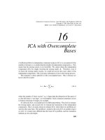
Fig. 7.1
The original audio signals.
signals is a weighted sum of the speech signals emitted by the three speakers, which
we denote by ,and . We could express this as a linear equation:
(7.1)
(7.2)

(7.3)
where the with are some parameters that depend on the distances
of the microphones from the speakers. It would be very useful if you could now
estimate the original speech signals ,and , using only the recorded
signals . This is called the cocktail-party problem. For the time being, we omit
any time delays or other extra factors from our simplified mixing model. A more
detailed discussion of the cocktail-party problem can be found later in Section 24.2.
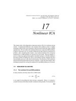
As an illustration, consider the waveforms in Fig. 7.1 and Fig. 7.2. The original
speech signals could look something like those in Fig. 7.1, and the mixed signals
could look like those in Fig. 7.2. The problem is to recover the “source” signals in
Fig. 7.1 using only the data in Fig. 7.2.
Actually, if we knew the mixing parameters , we could solve the linear equation
in (7.1) simply by inverting the linear system. The point is, however, that here we
know neither the nor the , so the problem is considerably more difficult.
One approach to solving this problem would be to use some information on
the statistical properties of the signals to estimate both the and the .
Actually, and perhaps surprisingly, it turns out that it is enough to assume that
MOTIVATION
149
0 500 1000 1500 2000 2500 3000
−1
0
1
0 500 1000 1500 2000 2500 3000
−2
0
2
0 500 1000 1500 2000 2500 3000
−1
0

1
2
Fig. 7.2
The observed mixtures of the original signals in Fig. 7.1.
0 500 1000 1500 2000 2500 3000
−5
0
5
10
0 500 1000 1500 2000 2500 3000
−5
0
5
0 500 1000 1500 2000 2500 3000
−5
0
5
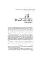
Fig. 7.3
The estimates of the original signals, obtained using only the observed signals in
Fig. 7.2. The original signals were very accurately estimated, up to multiplicative signs.
150
WHAT IS INDEPENDENT COMPONENT ANALYSIS?
,and are, at each time instant , statistically independent.This
is not an unrealistic assumption in many cases, and it need not be exactly true in
practice. Independent component analysis can be used to estimate the based on
the information of their independence, and this allows us to separate the three original
signals, , ,and , from their mixtures, , ,and .
Figure 7.3 gives the three signals estimated by the ICA methods discussed in the
next chapters. As can be seen, these are very close to the original source signals
(the signs of some of the signals are reversed, but this has no significance.) These

signals were estimated using only the mixtures in Fig. 7.2, together with the very
weak assumption of the independence of the source signals.
Independent component analysis was originally developed to deal with problems
that are closely related to the cocktail-party problem. Since the recent increase of
interest in ICA, it has become clear that this principle has a lot of other interesting
applications as well, several of which are reviewed in Part IV of this book.
Consider, for example, electrical recordings of brain activity as given by an
electroencephalogram (EEG). The EEG data consists of recordings of electrical
potentials in many different locations on the scalp. These potentials are presumably
generated by mixing some underlying components of brain and muscle activity.
This situation is quite similar to the cocktail-party problem: we would like to find
the original components of brain activity, but we can only observe mixtures of the
components. ICA can reveal interesting information on brain activity by giving
access to its independent components. Such applications will be treated in detail in
Chapter 22. Furthermore, finding underlying independent causes is a central concern
in the social sciences, for example, econometrics. ICA can be used as an econometric
tool as well; see Section 24.1.
Another, very different application of ICA is feature extraction. A fundamental
problem in signal processing is to find suitable representations for image, audio or
other kind of data for tasks like compression and denoising. Data representations
are often based on (discrete) linear transformations. Standard linear transformations
widely used in image processing are, for example, the Fourier, Haar, and cosine
transforms. Each of them has its own favorable properties.
It would be most useful to estimate the linear transformation from the data itself,
in which case the transform could be ideally adapted to the kind of data that is
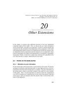
being processed. Figure 7.4 shows the basis functions obtained by ICA from patches
of natural images. Each image window in the set of training images would be
a superposition of these windows so that the coefficient in the superposition are
independent, at least approximately. Feature extraction by ICA will be explained in
more detail in Chapter 21.

All of the applications just described can actually be formulated in a unified
mathematical framework, that of ICA. This framework will be defined in the next
section.
DEFINITION OF INDEPENDENT COMPONENT ANALYSIS
151
Fig. 7.4
Basis functions in ICA of natural images. These basis functions can be considered
as the independent features of images. Every image window is a linear sum of these windows.
7.2 DEFINITION OF INDEPENDENT COMPONENT ANALYSIS
7.2.1 ICA as estimation of a generative model
To rigorously define ICA, we can use a statistical “latent variables” model. We
observe random variables , which are modeled as linear combinations of
random variables :
for all (7.4)
where the are some real coefficients. By definition, the are
statistically mutually independent.
This is the basic ICA model. The ICA model is a generative model, which means
that it describes how the observed data are generated by a process of mixing the
components . The independent components (often abbreviated as ICs) are latent
variables, meaning that they cannot be directly observed. Also the mixing coefficients
are assumed to be unknown. All we observe are the random variables ,andwe
must estimate both the mixing coefficients and the ICs using the . This must
be done under as general assumptions as possible.
Note that we have here dropped the time index that was used in the previous
section. This is because in this basic ICA model, we assume that each mixture as
well as each independent component is a random variable, instead of a proper time
signal or time series. The observed values , e.g., the microphone signals in the
152
WHAT IS INDEPENDENT COMPONENT ANALYSIS?
cocktail party problem, are then a sample of this random variable. We also neglect

any time delays that may occur in the mixing, which is why this basic model is often
called the instantaneous mixing model.
ICA is very closely related to the method called blind source separation (BSS) or
blind signal separation. A “source” means here an original signal, i.e., independent
component, like the speaker in the cocktail-party problem. “Blind” means that we
know very little, if anything, of the mixing matrix, and make very weak assumptions
on the source signals. ICA is one method, perhaps the most widely used, for
performing blind source separation.
It is usually more convenient to use vector-matrix notation instead of the sums
as in the previous equation. Let us denote by the random vector whose elements
are the mixtures , and likewise by the random vector with elements
. Let us denote by the matrix with elements . (Generally, bold
lowercase letters indicate vectors and bold uppercase letters denote matrices.) All
vectors are understood as column vectors; thus , or the transpose of ,isarow
vector. Using this vector-matrix notation, the mixing model is written as
(7.5)
Sometimes we need the columns of matrix
; if we denote them by the model
can also be written as
(7.6)
The definition given here is the most basic one, and in Part II of this book,
we will essentially concentrate on this basic definition. Some generalizations and
modifications of the definition will be given later (especially in Part III), however.
For example, in many applications, it would be more realistic to assume that there
is some noise in the measurements, which would mean adding a noise term in the
model (see Chapter 15). For simplicity, we omit any noise terms in the basic model,
since the estimation of the noise-free model is difficult enough in itself, and seems to
be sufficient for many applications. Likewise, in many cases the number of ICs and
observed mixtures may not be equal, which is treated in Section 13.2 and Chapter 16,
and the mixing might be nonlinear, which is considered in Chapter 17. Furthermore,

let us note that an alternative definition of ICA that does not use a generative model
will be given in Chapter 10.
7.2.2 Restrictions in ICA
To make sure that the basic ICA model just given can be estimated, we have to make
certain assumptions and restrictions.
1. The independent components are assumed statistically independent.
This is the principle on which ICA rests. Surprisingly, not much more than this
assumption is needed to ascertain that the model can be estimated. This is why ICA
is such a powerful method with applications in many different areas.
DEFINITION OF INDEPENDENT COMPONENT ANALYSIS
153
Basically, random variables are said to be independent if information
on the value of does not give any information on the value of for .
Technically, independence can be defined by the probability densities. Let us denote
by the joint probability density function (pdf) of the , and by
the marginal pdf of , i.e., the pdf of when it is considered alone. Then we say
that the are independent if and only if the joint pdf is factorizable in the following
way:
(7.7)
For more details, see Section 2.3.
2. The independent components must have nongaussian distributions.
Intuitively, one can say that the gaussian distributions are “too simple”. The higher-
order cumulants are zero for gaussian distributions, but such higher-order information
is essential for estimation of the ICA model, as will be seen in Section 7.4.2. Thus,
ICA is essentially impossible if the observed variables have gaussian distributions.
The case of gaussian components is treated in more detail in Section 7.5 below.
Note that in the basic model we do not assume that we know what the nongaussian
distributions of the ICs look like; if they are known, the problem will be considerably
simplified. Also, note that a completely different class of ICA methods, in which the
assumption of nongaussianity is replaced by some assumptions on the time structure

of the signals, will be considered later in Chapter 18.
3. For simplicity, we assume that the unknown mixing matrix is square.
In other words, the number of independent components is equal to the number of
observed mixtures. This assumption can sometimes be relaxed, as explained in
Chapters 13 and 16. We make it here because it simplifies the estimation very much.
Then, after estimating the matrix
, we can compute its inverse, say , and obtain
the independent components simply by
(7.8)
It is also assumed here that the mixing matrix is invertible. If this is not the case,
there are redundant mixtures that could be omitted, in which case the matrix would
not be square; then we find again the case where the number of mixtures is not equal
to the number of ICs.
Thus, under the preceding three assumptions (or at the minimum, the two first
ones), the ICA model is identifiable, meaning that the mixing matrix and the ICs
can be estimated up to some trivial indeterminacies that will be discussed next. We
will not prove the identifiability of the ICA model here, since the proof is quite
complicated; see the end of the chapter for references. On the other hand, in the next
chapter we develop estimation methods, and the developments there give a kind of a
nonrigorous, constructive proof of the identifiability.
154
WHAT IS INDEPENDENT COMPONENT ANALYSIS?
7.2.3 Ambiguities of ICA
In the ICA model in Eq. (7.5), it is easy to see that the following ambiguities or
indeterminacies will necessarily hold:
1. We cannot determine the variances (energies) of the independent components.
The reason is that, both and being unknown, any scalar multiplier in one of the
sources could always be canceled by dividing the corresponding column of
by the same scalar, say :
(7.9)

As a consequence, we may quite as well fix the magnitudes of the independent
components. Since they are random variables, the most natural way to do this is to
assume that each has unit variance: . Then the matrix will be adapted
in the ICA solution methods to take into account this restriction. Note that this still
leaves the ambiguity of the sign: we could multiply an independent component by
without affecting the model. This ambiguity is, fortunately, insignificant in most
applications.
2. We cannot determine the order of the independent components.
The reason is that, again both and being unknown, we can freely change the
order of the terms in the sum in (7.6), and call any of the independent components
the first one. Formally, a permutation matrix and its inverse can be substituted in
the model to give . The elements of are the original independent
variables
, but in another order. The matrix is just a new unknown mixing
matrix, to be solved by the ICA algorithms.
7.2.4 Centering the variables
Without loss of generality, we can assume that both the mixture variables and the
independent components have zero mean. This assumption simplifies the theory and
algorithms quite a lot; it is made in the rest of this book.
If the assumption of zero mean is not true, we can do some preprocessing to make
it hold. This is possible by centering the observable variables, i.e., subtracting their
sample mean. This means that the original mixtures, say
are preprocessed by
(7.10)
before doing ICA. Thus the independent components are made zero mean as well,
since
(7.11)
The mixing matrix, on the other hand, remains the same after this preprocessing, so
we can always do this without affecting the estimation of the mixing matrix. After
ILLUSTRATION OF ICA

155
Fig. 7.5
The joint distribution of the independent components and with uniform
distributions. Horizontal axis:
, vertical axis: .
estimating the mixing matrix and the independent components for the zero-mean
data, the subtracted mean can be simply reconstructed by adding to the
zero-mean independent components.
7.3 ILLUSTRATION OF ICA
To illustrate the ICA model in statistical terms, consider two independent components
that have the following uniform distributions:
if
otherwise
(7.12)
The range of values for this uniform distribution were chosen so as to make the
mean zero and the variance equal to one, as was agreed in the previous section. The
joint density of and is then uniform on a square. This follows from the basic
definition that the joint density of two independent variables is just the product of
their marginal densities (see Eq. (7.7)): we simply need to compute the product. The
joint density is illustrated in Fig. 7.5 by showing data points randomly drawn from
this distribution.
Now let us mix these two independent components. Let us take the following
mixing matrix:
(7.13)
156
WHAT IS INDEPENDENT COMPONENT ANALYSIS?
Fig. 7.6
The joint distribution of the observed mixtures and . Horizontal axis: ,
vertical axis:
. (Not in the same scale as Fig. 7.5.)

This gives us two mixed variables, and . It is easily computed that the mixed
data has a uniform distribution on a parallelogram, as shown in Fig. 7.6. Note that
the random variables and are not independent anymore; an easy way to see this
is to consider whether it is possible to predict the value of one of them, say , from
the value of the other. Clearly, if attains one of its maximum or minimum values,
then this completely determines the value of . They are therefore not independent.
(For variables and the situation is different: from Fig. 7.5 it can be seen that
knowing the value of does not in any way help in guessing the value of .)
The problem of estimating the data model of ICA is now to estimate the mixing
matrix using only information contained in the mixtures and . Actually, from
Fig. 7.6 you can see an intuitive way of estimating :Theedges of the parallelogram
are in the directions of the columns of . This means that we could, in principle,
estimate the ICA model by first estimating the joint density of and ,andthen
locating the edges. So, the problem seems to have a solution.
On the other hand, consider a mixture of ICs with a different type of distribution,
called supergaussian (see Section 2.7.1). Supergaussian random variables typically
have a pdf with a peak a zero. The marginal distribution of such an IC is given in
Fig. 7.7. The joint distribution of the original independent components is given in
Fig. 7.8, and the mixtures are shown in Fig. 7.9. Here, we see some kind of edges,
but in very different places this time.
In practice, however, locating the edges would be a very poor method because it
only works with variables that have very special distributions. For most distributions,
such edges cannot be found; we use only for illustration purposes distributions that
visually show edges. Moreover, methods based on finding edges, or other similar
heuristic methods, tend to be computationally quite complicated, and unreliable.
ILLUSTRATION OF ICA
157
Fig. 7.7
The density of one supergaussian independent component. The gaussian density i
give by the dashed line for comparison.

Fig. 7.8
The joint distribution of the independent components and with supergaussian
distributions. Horizontal axis:
, vertical axis: .
s
n
158
WHAT IS INDEPENDENT COMPONENT ANALYSIS?
Fig. 7.9
The joint distribution of the observed mixtures and , obtained from super-
gaussian independent components. Horizontal axis:
, vertical axis: .
What we need is a method that works for any distributions of the independent
components, and works fast and reliably. Such methods are the main subject of this
book, and will be presented in Chapters 8–12. In the rest of this chapter, however,
we discuss the connection between ICA and whitening.
7.4 ICA IS STRONGER THAT WHITENING
Given some random variables, it is straightforward to linearly transform them into
uncorrelated variables. Therefore, it would be tempting to try to estimate the indepen-
dent components by such a method, which is typically called whitening or sphering,
and often implemented by principal componentanalysis. In this section, we show that
this is not possible, and discuss the relation between ICA and decorrelation methods.
It will be seen that whitening is, nevertheless, a useful preprocessing technique for
ICA.
7.4.1 Uncorrelatedness and whitening
A weaker form of independence is uncorrelatedness. Here we review briefly the
relevant definitions that were already encountered in Chapter 2.
Two random variables and are said to be uncorrelated, if their covariance is
zero:
cov (7.14)

ICA IS STRONGER THAT WHITENING
159
In this book, all random variables are assumed to have zero mean, unless otherwise
mentioned. Thus, covariance is equal to correlation corr ,and
uncorrelatedness is the same thing as zero correlation (see Section 2.2).
1
If random variables are independent, they are uncorrelated. This is because if the
and are independent, then for any two functions, and ,wehave
(7.15)
see Section 2.3. Taking and , we see that this implies
uncorrelatedness.
On the other hand, uncorrelatedness does not imply independence. For example,
assume that are discrete valued and follow such a distribution that the pair
are with probability equal to any of the following values:
and .Then and are uncorrelated, as can be simply calculated. On the
other hand,
(7.16)
so the condition in Eq. (7.15) is violated, and the variables cannot be independent.
A slightly stronger property than uncorrelatedness is whiteness. Whiteness of a
zero-mean random vector, say , means that its components are uncorrelated and
their variances equal unity. In other words, the covariance matrix (as well as the
correlation matrix) of equals the identity matrix:
(7.17)
Consequently, whitening means that we linearly transform the observed data vector
by linearly multiplying it with some matrix
(7.18)
so that we obtain a new vector that is white. Whitening is sometimes called
sphering.
A whitening transformation is always possible. Some methods were reviewed in
Chapter 6. One popular method for whitening is to use the eigenvalue decomposition

(EVD) of the covariance matrix
(7.19)
where is the orthogonal matrix of eigenvectors of and is the diagonal
matrix of its eigenvalues, diag . Whitening can now be done by the
whitening matrix
(7.20)
1
In statistical literature, correlation is often defined as a normalized version of covariance. Here, we
use this simpler definition that is more widely spread in signal processing. In any case, the concept of
uncorrelatedness is the same.
160
WHAT IS INDEPENDENT COMPONENT ANALYSIS?
where the matrix is computed by a simple componentwise operation as
diag . A whitening matrix computed this way is denoted
by
or . Alternatively, whitening can be performed in connection
with principal component analysis, which gives a related whitening matrix. For
details, see Chapter 6.
7.4.2 Whitening is only half ICA
Now, suppose that the data in the ICA model is whitened, for example, by the matrix
given in (7.20). Whitening transforms the mixing matrix into a new one, .Wehave
from (7.5) and (7.18)
(7.21)
One could hope that whitening solves the ICA problem, since whiteness or uncor-
relatedness is related to independence. This is, however, not so. Uncorrelatedness
is weaker than independence, and is not in itself sufficient for estimation of the ICA
model. To see this, consider an orthogonal transformation of :
(7.22)
Due to the orthogonality of ,wehave
(7.23)

In other words, is white as well. Thus, we cannot tell if the independent components
are given by or using the whiteness property alone. Since could be any
orthogonal transformation of , whitening gives the ICs only up to an orthogonal
transformation. This is not sufficient in most applications.
On the other hand, whitening is useful as a preprocessing step in ICA. The utility
of whitening resides in the fact that the new mixing matrix is orthogonal.
This can be seen from
(7.24)
This means that we can restrict our search for the mixing matrix to the space of
orthogonal matrices. Instead of having to estimate the parameters that are the
elements of the original matrix , we only need to estimate an orthogonal mixing
matrix . An orthogonal matrix contains degrees of freedom. For
example, in two dimensions, an orthogonal transformation is determined by a single
angle parameter. In larger dimensions, an orthogonal matrix contains only about half
of the number of parameters of an arbitrary matrix.
Thus one can say that whitening solves half of the problem of ICA. Because
whitening is a very simple and standard procedure, much simpler than any ICA
algorithms, it is a good idea to reduce the complexity of the problem this way. The
remaining half of the parameters has to be estimated by some other method; several
will be introduced in the next chapters.
WHY GAUSSIAN VARIABLES ARE FORBIDDEN
161
Fig. 7.10
The joint distribution of the whitened mixtures of uniformly distributed indepen-
dent components.
A graphical illustration of the effect of whitening can be seen in Fig. 7.10, in
which the data in Fig. 7.6 has been whitened. The square defining the distribution is
now clearly a rotated version of the original square in Fig. 7.10. All that is left is the
estimation of a single angle that gives the rotation.
In many chapters of this book, we assume that the data has been preprocessed by

whitening, in which case we denote the data by . Even in cases where whitening
is not explicitly required, it is recommended, since it reduces the number of free
parameters and considerably increases the performance of the methods, especially
with high-dimensional data.
7.5 WHY GAUSSIAN VARIABLES ARE FORBIDDEN
Whitening also helps us understand why gaussian variables are forbidden in ICA.
Assume that the joint distribution of two ICs, and , is gaussian. This means that
their joint pdf is given by
(7.25)
(For more information on the gaussian distribution, see Section 2.5.) Now, assume
that the mixing matrix is orthogonal. For example, we could assume that this is
so because the data has been whitened. Using the classic formula of transforming
pdf’s in (2.82), and noting that for an orthogonal matrix holds, we get
162
WHAT IS INDEPENDENT COMPONENT ANALYSIS?
Fig. 7.11
The multivariate distribution of two independent gaussian variables.
the joint density of the mixtures and as density is given by
(7.26)
Due to the orthogonality of ,wehave and ; note that
if is orthogonal, so is . Thus we have
(7.27)
and we see that the orthogonal mixing matrix does not change the pdf, since it does
not appear in this pdf at all. The original and mixed distributions are identical.
Therefore, there is no way how we could infer the mixing matrix from the mixtures.
The phenomenon that the orthogonal mixing matrix cannot be estimated for gaus-
sian variables is related to the property that uncorrelated jointly gaussian variables are
necessarily independent(see Section 2.5). Thus, the information on the independence
of the components does not get us any further than whitening.
Graphically, we can see this phenomenon by plotting the distribution of the or-

thogonal mixtures, which is in fact the same as the distribution of the ICs. This
distribution is illustrated in Fig. 7.11. The figure shows that the density is rotation-
ally symmetric. Therefore, it does not contain any information on the directions of
the columns of the mixing matrix . This is why cannot be estimated.
Thus, in the case of gaussian independent components, we can only estimate the
ICA model up to an orthogonal transformation. In other words, the matrix is not
identifiable for gaussian independent components. With gaussian variables, all we
can do is whiten the data. There is some choice in the whitening procedure, however;
PCA is the classic choice.
CONCLUDING REMARKS AND REFERENCES
163
What happens if we try to estimate the ICA model and some of the components
are gaussian, some nongaussian? In this case, we can estimate all the nongaussian
components, but the gaussian components cannot be separated from each other. In
other words, some of the estimated components will be arbitrary linear combinations
of the gaussian components. Actually, this means that in the case of just one gaussian
component, we can estimate the model, because the single gaussian component does
not have any other gaussian components that it could be mixed with.
7.6 CONCLUDING REMARKS AND REFERENCES
ICA is a very general-purpose statistical technique in which observed random data are
expressed as a linear transform of components that are statistically independent from
each other. In this chapter, we formulated ICA as the estimation of a generative model,
with independent latent variables. Such a decomposition is identifiable, i.e., well
defined, if the independent components are nongaussian (except for perhaps one). To
simplify the estimation problem, we can begin by whitening the data. This estimates
part of the parameters, but leaves an orthogonal transformation unspecified. Using
the higher-order information contained in nongaussian variables, we can estimate
this orthogonal transformation as well.
Practical methods for estimating the ICA model will be treated in the rest of Part II.
A simple approach based on finding the maxima of nongaussianity is presented first

in Chapter 8. Next, the classic maximum likelihood estimation method is applied on
ICA in Chapter 9. An information-theoretic framework that also shows a connection
between the previous two is given by mutual information in Chapter 10. Some
further methods are considered in Chapters 11 and 12. Practical considerations on
the application of ICA methods, in particular on the preprocessing of the data, are
treated in Chapter 13. The different ICA methods are compared with each other, and
the choice of the “best” method is considered in Chapter 14, which concludes Part II.
The material that we treated in this chapter can be considered classic. The ICA
model was first defined as herein in [228]; somewhat related developments were given
in [24]. The identifiability is treated in [89, 423]. Whitening was proposed in [61] as
well. In addition to this research in signal processing, a parallel neuroscientific line
of research developed ICA independently. This was started by [26, 27, 28], being
more qualitative in nature. The first quantitative results in this area were proposed
in [131], and in [335], a model that is essentially equivalent to the noisy version
of the ICA model (see Chapter 15) was proposed. More on the history of ICA
can be found in Chapter 1, as well as in [227]. For recent reviews on ICA, see
[10, 65, 201, 267, 269, 149]. A shorter tutorial text is in [212].
164
Problems
matrix for , given by (7.20).
7.2 Show that two (zero-mean) random variables that have a jointly gaussian dis-
tribution are independent if and only if they are uncorrelated. (Hint: The pdf can
be found in (2.68). Uncorrelatedness means that the covariance matrix is diagonal.
Show that this implies that the joint pdf can be factorized.)
7.3 If both and could be observed, how would you estimate the ICA model?
(Assume there is some noise in the data as well.)
7.4 Assume that the data is multiplied by a matrix . Does this change the
independent components?
7.5 In our definition, the signs of the independent components are left undeter-
mined. How could you complement the definition so that they are determined as

well?
7.6 Assume that there are more independent components than observed mixtures.
Assume further that we have been able to estimate the mixing matrix. Can we recover
the values of the independent components? What if there are more observed mixtures
than ICs?
Computer assignments
7.1 Generate samples of two independent components that follow a Laplacian
distribution (see Eq. 2.96). Mix them with three different random mixing matrices.
in
the plots? Do the same for ICs that are obtained by taking absolute values of gaussian
random variables.
7.2 Generate samples of two independent gaussian random variables. Mix them
with a random mixing matrix. Compute a whitening matrix. Compute the product
of the whitening matrix and the mixing matrix. Show that this is almost orthogonal.
Why is it not exactly orthogonal?

Plot the distributions of the observed mixtures. Can you see the matrix
WHAT IS INDEPENDENT COMPONENT ANALYSIS?
7.1 Show that given a random vector , there is only one symmetric positive
semidefinite whitening