Tài liệu Independent component analysis P12 pdf

12
ICA by Nonlinear
Decorrelation and
Nonlinear PCA
This chapter starts by reviewing some of the early research efforts in independent
component analysis (ICA), especially the technique based on nonlinear decorrelation,
that was successfully used by Jutten, H
´
erault, and Ans to solve the first ICA problems.
Today, this work is mainly of historical interest, because there exist several more
efficient algorithms for ICA.
Nonlinear decorrelation can be seen as an extension of second-order methods
such as whitening and principal component analysis (PCA). These methods give
components that are uncorrelated linear combinations of input variables, as explained
in Chapter 6. We will show that independent components can in some cases be found
as nonlinearly uncorrelated linear combinations. The nonlinear functions used in
this approach introduce higher order statistics into the solution method, making ICA
possible.
We then show how the work on nonlinear decorrelation eventually lead to the
Cichocki-Unbehauen algorithm, which is essentially the same as the algorithm that
we derived in Chapter 9 using the natural gradient. Next, the criterion of nonlinear
decorrelation is extended and formalized to the theory of estimating functions, and
the closely related EASI algorithm is reviewed.
Another approach to ICA that is related to PCA is the so-called nonlinear PCA.
A nonlinear representation is sought for the input data that minimizes a least mean-
square error criterion. For the linear case, it was shown in Chapter 6 that principal
components are obtained. It turns out that in some cases the nonlinear PCA approach
gives independent components instead. We review the nonlinear PCA criterion and
show its equivalence to other criteria like maximum likelihood (ML). Then, two
typical learning rules introduced by the authors are reviewed, of which the first one
239

Independent Component Analysis. Aapo Hyv
¨
arinen, Juha Karhunen, Erkki Oja
Copyright
 2001 John Wiley & Sons, Inc.
ISBNs: 0-471-40540-X (Hardback); 0-471-22131-7 (Electronic)
240
ICA BY NONLINEAR DECORRELATION AND NONLINEAR PCA
is a stochastic gradient algorithm and the other one a recursive least mean-square
algorithm.
12.1 NONLINEAR CORRELATIONS AND INDEPENDENCE
The correlation between two random variables and was discussed in detail in
Chapter 2. Here we consider zero-mean variables only, so correlation and covariance
are equal. Correlation is related to independence in such a way that independent
variables are always uncorrelated. The opposite is not true, however: the variables
can be uncorrelated, yet dependent. An example is a uniform density in a rotated
square centered at the origin of the space, see e.g. Fig. 8.3. Both and
are zero mean and uncorrelated, no matter what the orientation of the square, but
they are independent only if the square is aligned with the coordinate axes. In some
cases uncorrelatedness does imply independence, though; the best example is the
case when the density of is constrained to be jointly gaussian.
Extending the concept of correlation, we here define the nonlinear correlation of
the random variables and as E . Here, and are two
functions, of which at least one is nonlinear. Typical examples might be polynomials
of degree higher than 1, or more complex functions like the hyperbolic tangent. This
means that one or both of the random variables are first transformed nonlinearly to
new variables and then the usual linear correlation between these new
variables is considered.
The question now is: Assuming that and are nonlinearly decorrelated in the
sense

E (12.1)
can we say something about their independence? We would hope that by making
this kind of nonlinear correlation zero, independence would be obtained under some
additional conditions to be specified.
There is a general theorem (see, e.g., [129]) stating that and are independent
if and only if
E E E (12.2)
for all continuous functions and that are zero outside a finite interval. Based
on this, it seems very difficult to approach independence rigorously, because the
functions and are almost arbitrary. Some kind of approximations are needed.
This problem was considered by Jutten and H
´
erault [228]. Let us assume that
and are smooth functions that have derivatives of all orders in a neighborhood
NONLINEAR CORRELATIONS AND INDEPENDENCE
241
of the origin. They can be expanded in Taylor series:
where is shorthand for the coefficients of the th powers in the series.
The product of the functions is then
(12.3)
and condition (12.1) is equivalent to
E E (12.4)
Obviously, a sufficient condition for this equation to hold is
E (12.5)
for all indices appearing in the series expansion (12.4). There may be other
solutions in which the higher order correlations are not zero, but the coefficients
happen to be just suitable to cancel the terms and make the sum in (12.4) exactly
equal to zero. For nonpolynomial functions that have infinite Taylor expansions, such
spurious solutions can be considered unlikely (we will see later that such spurious
solutions do exist but they can be avoided by the theory of ML estimation).

Again, a sufficient condition for (12.5) to hold is that the variables and are
independent and one of E E is zero. Let us require that E for all
powers appearing in its series expansion. But this is only possible if is an odd
function; then the Taylor series contains only odd powers , and the powers
in Eq. (12.5) will also be odd. Otherwise, we have the case that even moments of
like the variance are zero, which is impossible unless is constant.
To conclude, a sufficient (but not necessary) condition for the nonlinear uncorre-
latedness (12.1) to hold is that and are independent, and for one of them, say
, the nonlinearity is an odd function such that has zero mean.
The preceding discussion is informal but should make it credible that nonlinear
correlations are useful as a possible general criterion for independence. Several things
have to be decided in practice: the first one is how to actually choose the functions
. Is there some natural optimality criterion that can tell us that some functions
242
ICA BY NONLINEAR DECORRELATION AND NONLINEAR PCA
yx
1
21
12
-m
-m
2
1
2
x y
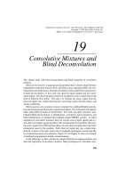
Fig. 12.1
The basic feedback circuit for the H
´
erault-Jutten algorithm. The element marked
with

is a summation
are better than some other ones? This will be answered in Sections 12.3 and 12.4.
The second problem is how we could solve Eq. (12.1), or nonlinearly decorrelate two
variables . This is the topic of the next section.
12.2 THE H
´
ERAULT-JUTTEN ALGORITHM
Consider the ICA model . Let us first look at a case, which was
considered by H
´
erault, Jutten and Ans [178, 179, 226] in connection with the blind
separation of two signals from two linear mixtures. The model is then
H
´
erault and Jutten proposed the feedback circuit shown in Fig. 12.1 to solve the prob-
lem. The initial outputs are fed back to the system, and the outputs are recomputed
until an equilibrium is reached.
From Fig. 12.1 we have directly
(12.6)
(12.7)
Before inputting the mixture signals to the network, they were normalized to
zero mean, which means that the outputs also will have zero means. Defining a
matrix with off-diagonal elements and diagonal elements equal to zero,
these equations can be compactly written as
Thus the input-output mapping of the network is
(12.8)
THE CICHOCKI-UNBEHAUEN ALGORITHM
243
Note that from the original ICA model we have , provided that is
invertible. If ,then becomes equal to . However, the problem in blind

separation is that the matrix is unknown.
The solution that Jutten and H
´
erault introduced was to adapt the two feedback
coefficients so that the outputs of the network become independent.
Then the matrix has been implicitly inverted and the original sources have been
found. For independence, they used the criterion of nonlinear correlations. They
proposed the following learning rules:
(12.9)
(12.10)
with
the learning rate. Both functions are odd functions; typically, the
functions
were used, although the method also seems to work for or sign .
Now, if the learning converges, then the right-hand sides must be zero on average,
implying
E E
Thus independence has hopefully been attained for the outputs . A stability
analysis for the H
´
erault-Jutten algorithm was presented by [408].
In the numerical computation of the matrix according to algorithm (12.9,12.10),
the outputs on the right-hand side must also be updated at each step of the
iteration. By Eq. (12.8), they too depend on , and solving them requires the
inversion of matrix . As noted by Cichocki and Unbehauen [84], this matrix
inversion may be computationally heavy, especially if this approach is extended to
more than two sources and mixtures. One way to circumvent this problem is to make
a rough approximation
that seems to work in practice.
Although the H

´
erault-Jutten algorithm was a very elegant pioneering solution to
the ICA problem, we know now that it has some drawbacks in practice. The algorithm
may work poorly or even fail to separate the sources altogether if the signals are badly
scaled or the mixing matrix is ill-conditioned. The number of sources that the method
can separate is severely limited. Also, although the local stability was shown in [408],
good global convergence behavior is not guaranteed.
12.3 THE CICHOCKI-UNBEHAUEN ALGORITHM
Starting from the H
´
erault-Jutten algorithm Cichocki, Unbehauen, and coworkers [82,
85, 84] derived an extension that has a much enhanced performance and reliability.
Instead of a feedback circuit like the H
´
erault-Jutten network in Fig. 12.1, Cichocki
244
ICA BY NONLINEAR DECORRELATION AND NONLINEAR PCA
and Unbehauen proposed a feedforward network with weight matrix , with the
mixture vector for input and with output . Now the dimensionality of the
problem can be higher than 2. The goal is to adapt the matrix so that the
elements of become independent. The learning algorithm for is as follows:
(12.11)
where
is the learning rate, is a diagonal matrix whose elements determine the
amplitude scaling for the elements of (typically, could be chosen as the unit
matrix ), and and are two nonlinear scalar functions; the authors proposed a
polynomial and a hyperbolic tangent. The notation means a column vector with
elements .
The argumentation showing that this algorithm will give independent components,
too, is based on nonlinear decorrelations. Consider the stationary solution of this

learning rule defined as the matrix for which E , with the expectation
taken over the density of the mixtures . For this matrix, the update is on the average
zero. Because this is a stochastic-approximation-typealgorithm(see Chapter 3), such
stationarity is a necessary condition for convergence. Excluding the trivial solution
,wemusthave
E
Especially, for the off-diagonal elements, this implies
E
(12.12)
which is exactly our definition of nonlinear decorrelation in Eq. (12.1) extended to
output signals . The diagonal elements satisfy
E
showing that the diagonal elements of matrix only control the amplitude scaling
of the outputs.
The conclusion is that if the learning rule converges to a nonzero matrix ,then
the outputs of the network must become nonlinearly decorrelated, and hopefully
independent. The convergence analysis has been performed in [84]; for general
principles of analyzing stochastic iteration algorithms like (12.11), see Chapter 3.
The justification for the Cichocki-Unbehauen algorithm (12.11) in the original
articles was based on nonlinear decorrelations, not on any rigorous cost functions
that would be minimized by the algorithm. However, it is interesting to note that
this algorithm, first appearing in the early 1990’s, is in fact the same as the popular
natural gradient algorithm introduced later by Amari, Cichocki, and Young [12] as
an extension to the original Bell-Sejnowski algorithm [36]. All we have to do is
choose as the unit matrix, the function as the linear function ,
and the function as a sigmoidal related to the true density of the sources. The
Amari-Cichocki-Young algorithm and the Bell-Sejnowski algorithm were reviewed
in Chapter 9 and it was shown how the algorithms are derived from the rigorous
maximum likelihood criterion. The maximum likelihood approach also tells us what
kind of nonlinearities should be used, as discussed in Chapter 9.

THE ESTIMATING FUNCTIONS APPROACH *
245
12.4 THE ESTIMATING FUNCTIONS APPR OACH *
Consider the criterion of nonlinear decorrelations being zero, generalized to
random
variables , shown in Eq. (12.12). Among the possible roots of
these equations are the source signals . When solving these in an algorithm
like the H
´
erault-Jutten algorithm or the Cichocki-Unbehauen algorithm, one in fact
solves the separating matrix
.
This notion was generalized and formalized by Amari and Cardoso [8] to the case
of estimating functions. Again, consider the basic ICA model ,
where is a true separating matrix (we use this special notation here to avoid any
confusion). An estimation function is a matrix-valued function such that
E (12.13)
This means that, taking the expectation with respect to the density of ,thetrue
separating matrices are roots of the equation. Once these are solved from Eq. (12.13),
the independent components are directly obtained.
Example 12.1 Given a set of nonlinear functions , with ,
and defining a vector function , a suitable estimating
function for ICA is
(12.14)
because obviously E
becomes diagonal when is a true separating matrix
and are independent and zero mean. Then the off-diagonal elements
become E E E . The diagonal matrix determines the
scales of the separated sources. Another estimating function is the right-hand side of
the learning rule (12.11),

There is a fundamental difference in the estimating function approach compared to
most of the other approaches to ICA: the usual starting point in ICA is a cost function
that somehow measures how independent or nongaussian the outputs are, and the
independent components are solved by minimizing the cost function. In contrast,
there is no such cost function here. The estimation function need not be the gradient
of any other function. In this sense, the theory of estimating functions is very general
and potentially useful for finding ICA algorithms. For a discussion of this approach
in connection with neural networks, see [328].
It is not a trivial question how to design in practice an estimation function so that
we can solve the ICA model. Even if we have two estimating functions that both
have been shaped in such a way that separating matrices are their roots, what is a
relevant measure to compare them? Statistical considerations are helpful here. Note
that in practice, the densities of the sources and the mixtures are unknown in
246
ICA BY NONLINEAR DECORRELATION AND NONLINEAR PCA
the ICA model. It is impossible in practice to solve Eq. (12.13) as such, because the
expectation cannot be formed. Instead, it has to be estimated using a finite sample of
. Denoting this sample by , we use the sample function
E
Its root is then an estimator for the true separating matrix. Obviously (see Chapter
4), the root is a function of the training sample, and it is
meaningful to consider its statistical properties like bias and variance. This gives a
measure of goodness for the comparison of different estimation functions. The best
estimating function is one that gives the smallest error between the true separating
matrix and the estimate .
A particularly relevant measure is (Fisher) efficiency or asymptotic variance, as
the size of the sample grows large (see Chapter 4). The goal is
to design an estimating function that gives the smallest variance, given the set of
observations . Then the optimal amount of information is extracted from the
training set.

The general result provided by Amari and Cardoso [8] is that estimating functions
of the form (12.14) are optimal in the sense that, given any estimating function ,
one can always find a better or at least equally good estimating function (in the sense
of efficiency) having the form
(12.15)
(12.16)
where is a diagonal matrix. Actually, the diagonal matrix has no effect on the
off-diagonal elements of which are the ones determining the independence
between ; the diagonal elements are simply scaling factors.
The result shows that it is unnecessary to use a nonlinear function instead of
as the other one of the two functions in nonlinear decorrelation. Only one nonlinear
function , combined with , is sufficient. It is interesting that functions of exactly
the type naturally emerge as gradients of cost functions such as likelihood;
the question of how to choose the nonlinearity is also answered in that case. A
further example is given in the following section.
The preceding analysis is not related in any way to the practical methods for finding
the roots of estimating functions. Due to the nonlinearities, closed-form solutions do
not exist and numerical algorithms have to be used. The simplest iterative stochastic
approximation algorithm for solving the roots of has the form
(12.17)
with an appropriate learning rate. In fact, we now discover that the learning rules
(12.9), (12.10) and (12.11) are examples of this more general framework.
EQUIVARIANT ADAPTIVE SEPARATION VIA INDEPENDENCE
247
12.5 EQUIVARIANT ADAPTIVE SEPARATION VIA INDEPENDENCE
In most of the proposed approaches to ICA, the learning rules are gradient descent
algorithms of cost (or contrast) functions. Many cases have been covered in previous
chapters. Typically, the cost function has the form
E , with
some scalar function, and usually some additional constraints are used. Here again

, and the form of the function and the probability density of determine
the shape of the contrast function .
It is easy to show (see the definition of matrix and vector gradients in Chapter 3)
that
E E (12.18)
where is the gradient of .If is square and invertible, then
and we have
E (12.19)
For appropriate nonlinearities , these gradients are estimating functions in
the sense that the elements of must be statistically independent when the gradient
becomes zero. Note also that in the form E , the first factor
has the shape of an optimal estimating function (except for the diagonal
elements); see eq. (12.15). Now we also know how the nonlinear function
can be determined: it is directly the gradient of the function appearing in the
original cost function.
Unfortunately, the matrix inversion in (12.19) is cumbersome. Matrix
inversion can be avoided by using the so-called natural gradient introduced by Amari
[4]. This is covered in Chapter 3. The natural gradient is obtained in this case by
multiplying the usual matrix gradient (12.19) from the right by matrix ,which
gives E . The ensuing stochastic gradient algorithm to minimize the cost
function is then
(12.20)
This learning rule again has the form of nonlinear decorrelations. Omitting the
diagonal elements in matrix in , the off-diagonal elements have the same
form as in the Cichocki-Unbehauen algorithm (12.11), with the two functions now
given by the linear function and the gradient .
This gradient algorithm can also be derived using the relative gradient introduced
by Cardoso and Hvam Laheld [71]. This approach is also reviewed in Chapter
3. Based on this, the authors developed their equivariant adaptive separation via
independence (EASI) learning algorithm. To proceed from (12.20) to the EASI

learning rule, an extra step must be taken. In EASI, as in many other learning
rules for ICA, a whitening preprocessing is considered for the mixture vectors
(see Chapter 6). We first transform linearly to whose elements have
248
ICA BY NONLINEAR DECORRELATION AND NONLINEAR PCA
unit variances and zero covariances: E . As also shown in Chapter 6, an
appropriate adaptation rule for whitening is
(12.21)
The ICA model using these whitened vectors instead of the original ones becomes
, and it is easily seen that the matrix is an orthogonal matrix (a rotation).
Thus its inverse which gives the separating matrix is also orthogonal. As in earlier
chapters, let us denote the orthogonal separating matrix by .
Basically, the learning rule for would be the same as (12.20). However, as
noted by [71], certain constraints must hold in any updating of if the orthogonality
is to be preserved at each iteration step. Let us denote the serial update for using
the learning rule (12.20), briefly, as , where now .
The orthogonality condition for the updated matrix becomes
where has been substituted. Assuming small, the first-order approxi-
mation gives the condition that ,or must be skew-symmetric. Applying
this condition to the relative gradient learning rule (12.20) for ,wehave
(12.22)
where now . Contrary to the learning rule (12.20), this learning rule also
takes care of the diagonal elements of in a natural way, without imposing
any conditions on them.
What is left now is to combine the two learning rules (12.21) and (12.22) into
just one learning rule for the global system separation matrix. Because
, this global separation matrix is . Assuming the same learning rates
for the two algorithms, a first order approximation gives
(12.23)
This is the EASI algorithm. It has the nice feature of combining both whitening

and separation into a single algorithm. A convergence analysis as well as some
experimental results are given in [71]. One can easily see the close connection to the
nonlinear decorrelation algorithm introduced earlier.
The concept of equivariance that forms part of the name of the EASI algorithm
is a general concept in statistical estimation; see, e.g., [395]. Equivariance of an
estimator means, roughly, that its performance does not depend on the actual value of
the parameter. In the context of the basic ICA model, this means that the ICs can be
estimated with the same performance what ever the mixing matrix may be. EASI was
one of the first ICA algorithms which was explicitly shown to be equivariant. In fact,
most estimators of the basic ICA model are equivariant. For a detailed discussion,
see [69].
NONLINEAR PRINCIPAL COMPONENTS
249
12.6 NONLINEAR PRINCIPAL COMPONENTS
One of the basic definitions of PCA was optimal least mean-square error compres-
sion, as explained in more detail in Chapter 6. Assuming a random
-dimensional
zero-mean vector , we search for a lower dimensional subspace such that the
residual error between and its orthogonal projection on the subspace is minimal,
averaged over the probability density of
. Denoting an orthonormal basis of this
subspace by , the projection of on the subspace spanned by the ba-
sis is .Now is the dimension of the subspace. The minimum
mean-square criterion for PCA is
minimize E (12.24)
A solution (although not the unique one) of this optimization problem is given by the
eigenvectors of the data covariance matrix E . Then the linear
factors in the sum become the principal components .
For instance, if is two-dimensional with a gaussian density, and we seek for a
one-dimensional subspace (a straight line passing through the center of the density),

then the solution is given by the principal axis of the elliptical density.
We now pose the question how this criterion and its solution are changed if a
nonlinearity is included in the criterion. Perhaps the simplest nontrivial nonlinear
extension is provided as follows. Assuming a set of scalar functions,
as yet unspecified, let us look at a modified criterion to be minimized with respect to
the basis vectors [232]:
E (12.25)
This criterion was first considered by Xu [461] who called it the “least mean-square
error reconstruction” (LMSER) criterion.
The only change with respect to (12.24) is that instead of the linear factors ,we
now have nonlinear functions of them in the expansion that gives the approximation
to . In the optimal solution that minimizes the criterion ,such
factors might be termed nonlinear principal components. Therefore, the technique of
finding the basis vectors is here called “nonlinear principal component analysis”
(NLPCA).
It should be emphasized that practically always when a well-defined linear problem
is extended into a nonlinear one, many ambiguities and alternative definitions arise.
This is the case here, too. The term “nonlinear PCA” is by no means unique.
There are several other techniques, like the method of principal curves [167, 264]
or the nonlinear autoassociators [252, 325] that also give “nonlinear PCA”. In these
methods, the approximating subspace is a curved manifold, while the solution to the
problem posed earlier is still a linear subspace. Only the coefficients corresponding
to the principal components are nonlinear functions of . It should be noted that
250
ICA BY NONLINEAR DECORRELATION AND NONLINEAR PCA
minimizing the criterion (12.25) does not give a smaller least mean square error than
standard PCA. Instead, the virtue of this criterion is that it introduces higher-order
statistics in a simple manner via the nonlinearities .
Before going into any deeper analysis of (12.25), it may be instructive to see in
a simple special case how it differs from linear PCA and how it is in fact related to

ICA.
If the functions were linear, as in the standard PCA technique, and the number
of terms in the sum were equal to or the dimension of , then the representation
error always would be zero, as long as the weight vectors are chosen orthonormal.
For nonlinear functions , however, this is usually not true. Instead, in some
cases, at least, it turns out that the optimal basis vectors minimizing (12.25) will
be aligned with the independent components of the input vectors.
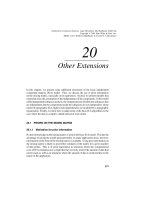
Example 12.2 Assume that is a two-dimensional random vector that has a uniform
density in a unit square that is not aligned with the coordinate axes , according to
Fig. 12.2. Then it is easily shown that the elements are uncorrelated and have
equal variances (equal to 1/3), and the covariance matrix of is therefore equal to
. Thus, except for the scaling by , vector is whitened (sphered). However,
the elements are not independent. The problem is to find a rotation of
such that the elements of the rotated vector are statistically independent. It is
obvious from Fig. 12.2 that the elements of must be aligned with the orientation of
the square, because then and only then the joint density is separable into the product
of the two marginal uniform densities.
Because of the whitening, we know that the rows of the separating matrix must
be orthogonal. This is seen by writing
E E (12.26)
Because the elements and are uncorrelated, it must hold that =0.
The solution minimizing the criterion (12.25), with orthogonal two-
dimensional vectors and a suitable nonlinearity, provides now
a rotation into independent components. This can be seen as follows. Assume that
is a very sharp sigmoid, e.g., , which is approximately the sign
function. The term in criterion (12.25) becomes
sign sign
Thus according to (12.25), each should be optimally represented by one of the four
possible points , with the signs depending on the angles between and
the basis vectors. Each choice of the two orthogonal basis vectors divides the square

of Fig. 12.2 into four quadrants, and by criterion (12.25), all the points in a given
quadrant must be represented in the least mean square sense by just one point; e.g.,
in the first quadrant where the angles between and the basis vectors are positive,
by the point . From Fig. 12.2, it can be seen that the optimal fit is obtained
THE NONLINEAR PCA CRITERION AND ICA
251
w
w
x
x
s
2
2
2
1
1
1
s
Fig. 12.2
A rotated uniform density
when the basis vectors are aligned with the axes , and the point is the
center of the smaller square bordered by the positive axes.
For further confirmation, it is easy to compute the theoretical value of the cost
function of Eq. (12.25) when the basis vectors and are arbitrary
orthogonal vectors [327]. Denoting the angle between and the axis in Fig.
12.2 by , we then have the minimal value of for the rotation ,and
then the lengths of the orthogonal vectors are equal to 0.5. These are the vectors
shown in Fig. 12.2.
In the preceding example, it was assumed that the density of is uniform. For
some other densities, the same effect of rotation into independent directions would

not be achieved. Certainly, this would not take place for gaussian densities with
equal variances, for which the criterion would be independent of
the orientation. Whether the criterion results in independent components, depends
strongly on the nonlinearities . A more detailed analysis of the criterion (12.25)
and its relation to ICA is given in the next section.
12.7 THE NONLINEAR PCA CRITERION AND ICA
Interestingly, for prewhitened data, it can be shown [236] that the original nonlinear
PCA criterion of Eq. (12.25) has an exact relationship with other contrast func-
252
ICA BY NONLINEAR DECORRELATION AND NONLINEAR PCA
tions like kurtosis maximization/minimization, maximum likelihood, or the so-called
Bussgang criteria. In the prewhitened case, we use instead of to denote the input
vector. Also, assume that in whitening, the dimension of has been reduced to that
of . We denote this dimension by . In this case, it has been shown before (see
Chapter 13) that matrix is and orthogonal: it holds .
First, it is convenient to change to matrix formulation. Denoting by
the matrix that has the basis vectors as rows, criterion (12.25) be-
comes
E (12.27)
The function
is a column vector with elements .We
can write now [236]
with . Therefore the criterion becomes
E (12.28)
This formulation of the NLPCA criterion can now be related to several other contrast
functions.
As the first case, choose as the odd quadratic function (the same for all )
if
if
Then the criterion (12.28) becomes

kurt
E E (12.29)
This statistic was discussed in Chapter 8. Note that because the input data has been
whitened, the variance E E , so in the kurtosis
kurt E E the second term is a constant and can be dropped
in kurtosis maximization/minimization. What remains is criterion (12.29). For this
function, minimizing the NLPCA criterion is exactly equivalent to minimizing the
sum of the kurtoses of .
As a second case, consider the maximum likelihood solution of the ICA model.
The maximum likelihood solution starts from the assumption that the density of ,
THE NONLINEAR PCA CRITERION AND ICA
253
due to independence, is factorizable: . Suppose we
have a large sample of input vectors available. It was shown in
Chapter 9 that the log-likelihood becomes
(12.30)
where the vectors
are the rows of matrix . In the case of a whitened
sample , the separating matrix will be orthogonal. Let us denote it
again by .Wehave
(12.31)
The second term in (12.30) is zero, because the determinant of the orthogonal matrix
is equal to one.
Because this is a maximization problem, we can multiply the cost function (12.31)
by the constant .Forlarge , this function tends to
E (12.32)
with .
From this, we can easily derive the connection between the NLPCA criterion
(12.28) and the ML criterion (12.32). In minimizing the sum (12.28), an arbi-
trary additive constant and a positive multiplicative constant can be trivially added.

Therefore, in the equivalence between the two criteria, we can consider the relation
(dropping the subscript from for convenience)
(12.33)
where and are some constants, yielding
(12.34)
This shows how to choose the function for any given density .
As the third case, the form of (12.28) is quite similar to the so-called Bussgang
cost function used in blind equalization (see [170, 171]). We use Lambert’s notation
and approach [256]. He chooses only one nonlinearity :
E
(12.35)
The function is the density of and its derivative. Lambert [256] also gives
several algorithms for minimizing this cost function. Note that now in the whitened
254
ICA BY NONLINEAR DECORRELATION AND NONLINEAR PCA
data case the variance of is equal to one and the function (12.35) is simply the score
function
Due to the equivalence of the maximum likelihood criterion to several other criteria
like infomax or entropic criteria, further equivalences of the NLPCA criterion with
these can be established. More details are given in [236] and Chapter 14.
12.8 LEARNING RULES FOR THE NONLINEAR PCA CRITERION
Once the nonlinearities
have been chosen, it remains to actually solve the
minimization problem in the nonlinear PCA criterion. Here we present the simplest
learning algorithms for minimizing either the original NLPCA criterion (12.25) or
the prewhitened criterion (12.28). The first algorithm, the nonlinear subspace rule, is
of the stochastic gradient descent type; this means that the expectation in the criterion
is dropped and the gradient of the sample function that only depends on the present
sample of the input vector ( or , respectively) is taken. This allows on-line learning
in which each input vector is used when it comes available and then discarded;

see Chapter 3 for more details. This algorithm is a nonlinear generalization of the
subspace rule for PCA, covered in Chapter 6. The second algorithm reviewed in this
section, the recursive least-squares learning rule,islikewise a nonlinear generalization
of the PAST algorithm for PCA covered in Chapter 6.
12.8.1 The nonlinear subspace rule
Let us first consider a stochastic gradient algorithm for the original cost function
(12.25), which in matrix form can be written as E .
This problem was considered by one of the authors [232, 233] as well as by Xu [461].
It was shown that the stochastic gradient algorithm is
(12.36)
where
(12.37)
is the residual error term and
diag (12.38)
There denotes the derivative of the function . We have made the simplifying
assumption here that all the functions are equal; a generalization to the
case of different functions would be straightforward but the notation would become
more cumbersome.
As motivated in more detail in [232], writing the update rule (12.36) for an
individual weight vector shows that the first term in the brackets on the right-hand
LEARNING RULES FOR THE NONLINEAR PCA CRITERION
255
side of (12.36) affects the update of weight vectors much less than the second term,
if the error is relatively small in norm compared to the input vector .Ifthefirst
term is omitted, then we obtain the following learning rule:
(12.39)
with the vector
(12.40)
Comparing this learning rule to the subspace rule for ordinary PCA, eq. (6.19)
in Chapter 6, we see that the algorithms are formally similar and become the same

if is a linear function. Both rules can be easily implemented in the one-layer PCA
network shown in Fig. 6.2 of Chapter 6; the linear outputs must only be
changed to nonlinear versions . This was the way the nonlinear
PCA learning rule was first introduced in [332] as one of the extensions to numerical
on-line PCA computation.
Originally, in [232] the criterion (12.25) and the learning scheme (12.39) were
suggested for signal separation, but the exact relation to ICA was not clear. Even
without prewhitening of the inputs , the method can separate signals to a certain
degree. However, if the inputs are whitened first, the separation performance is
greatly improved. The reason is that for whitened inputs, the criterion (12.25) and the
consequent learning rule are closely connected to well-known ICA objective (cost)
functions, as was shown in Section 12.7.
12.8.2 Convergence of the nonlinear subspace rule *
Let us consider the convergence and behavior of the learning rule in the case that the
ICA model holds for the data. This is a very specialized section that may be skipped.
The prewhitened form of the learning rule is
(12.41)
with now the vector
(12.42)
and white, thus E . We also have to assume that the ICA model holds,
i.e., there exists an orthogonal separating matrix such that
(12.43)
where the elements of are statistically independent. With whitening, the dimension
of has been reduced to that of ; thus both and are matrices.
To make further analysis easier, we proceed by making a linear transformation to
the learning rule (12.41): we multiply both sides by the orthogonal separating matrix
,giving
(12.44)
256
ICA BY NONLINEAR DECORRELATION AND NONLINEAR PCA

where we have used the fact that . Denoting for the moment
and using (12.43), we have
(12.45)
This equation has exactly the same form as the original one (12.41). Geometrically
the transformation by the orthogonal matrix simply means a coordinate change
to a new set of coordinates such that the elements of the input vector expressed in
these coordinates are statistically independent.
The goal in analyzing the learning rule (12.41) is to show that, starting from some
initial value, the matrix
will tend to the separating matrix . For the transformed
weight matrix in (12.45), this translates into the requirement that
should tend to the unit matrix or a permutation matrix. Then also would
tend to the vector , or a permuted version, with independent components.
However, it turns out that in the learning rule (12.45), the unit matrix or a per-
mutation matrix generally cannot be the asymptotic or steady state solution. This
is due to the scaling given by the nonlinearity . Instead, we can make the more
general requirement that tends to a diagonal matrix or a diagonal matrix times a
permutation matrix. In this case the elements of will become the elements
of the original source vector , in some order, multiplied by some numbers. In view
of the original problem, in which the amplitudes of the signals remain unknown,
this is actually no restriction, as independence is again attained.
To proceed, the difference equation (12.45) can be further analyzed by writing
down the corresponding averaged differential equation; for a discussion of the tech-
nique, see Chapter 3. The limit of convergence of (12.45) is among the asymptotically
stable solutions of the averaged differential equation. In practice, this also requires
that the learning rate is decreasing to zero at a suitable rate.
Now taking averages in (12.45) and also using the same symbol for
the continuous-time counterpart of the transformed weight matrix , we obtain
E E (12.46)
The expectations are over the (unknown) density of vector . Wearereadytostate

the main result of this section:
Theorem 12.1 In the matrix differential equation (12.46), assume the f ollowing:
1. The random vector has a symmetric density with E ;
2. The elements o f , denoted , are statistically independent;
3. The function is odd, i.e., for all , and at least twice
differentiable everywhere;
4. The function and the density of are such that the following conditions
hold for all :
E E E
(12.47)
LEARNING RULES FOR THE NONLINEAR PCA CRITERION
257
where the are scalars satisfying
E E (12.48)
5. Denoting
E (12.49)
E (12.50)
E (12.51)
E (12.52)
both eigenvalues of the matrix
(12.53)
have strictly negative real parts for all .
Then the matrix
(12.54)
is an asymptotically stable stationary point of (12.46), where satisfies Eq. (12.48).
The proof, as well as explanations of the rather technical conditions of the theorem,
are given in [327]. The main point is that the algorithm indeed converges to a diagonal
matrix, if the initial value is not too far from it. Transformingback to the original
learning rule (12.41) for , it follows that converges to a separating matrix.
Some special cases were given in [327]. For example, if the nonlinearity is chosen

as the simple odd polynomial
(12.55)
then all the relevant variables in the conditions of the theorem, for any probability
density, will become moments of . It can be shown (see exercises) that the stability
condition becomes
E E E (12.56)
Based on this, it can be shown that the linear function never gives asymptotic
stability, while the cubic function leads to asymptotic stability provided
that the density of satisfies
E E (12.57)
This expression is exactly the kurtosis or the fourth order cumulant of [319]. If
and only if the density is positively kurtotic (supergaussian), the stability condition
is satisfied for the cubic polynomial .
258
ICA BY NONLINEAR DECORRELATION AND NONLINEAR PCA
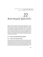
S1 S2 S3
S4 S5 S6
S7 S8 S9
Fig. 12.3
The original images.
Example 12.3 The learning rule was applied to a signal separation problem in [235].
Consider the 9 digital images shown in Fig. 12.3. They were linearly mixed with a
randomly chosen mixing matrix into 9 mixture images, shown in Fig. 12.4.
Whitening, shown in Fig. 12.5, is not able to separate the images. When the
learning rule (12.41) was applied to the mixtures with a nonlinearity and the
matrix was allowed to converge, it was able to separate the images as shown in
Fig. 12.6. In the figure, the images have been scaled to fit the gray levels in use; in
some cases, the sign has also been reversed to avoid image negatives.
12.8.3 The nonlinear recursive least-squares learning rule
It is also possible to effectively minimize the prewhitened NLPCA criterion (12.27)

using approximative recursive least-squares (RLS) techniques. Generally, RLS algo-
rithms converge clearly faster than their stochastic gradient counterparts, and achieve
a good final accuracy at the expense of a somewhat higher computational load. These
LEARNING RULES FOR THE NONLINEAR PCA CRITERION
259
M1 M2 M3
M4 M5 M6
M7 M8 M9
Fig. 12.4
The mixed images.
advantages are the result of the automatic determination of the learning rate parameter
from the input data, so that it becomes roughly optimal.
The basic symmetric algorithm for the prewhitened problem was derived by one of
the authors [347]. This is a nonlinear modification of the PAST algorithm introduced
by Yang for the standard linear PCA [466, 467]; the PAST algorithm is covered in
Chapter 6. Using index to denote the iteration step, the algorithm is
(12.58)
(12.59)
(12.60)
Tri (12.61)
(12.62)
(12.63)
The vector variables ,and and the matrix variable are
auxiliary variables, internal to the algorithm. As before, is the whitened input
260
ICA BY NONLINEAR DECORRELATION AND NONLINEAR PCA
W1 W2 −W3
−W4 W5 W6
−W7 −W8 −W9
Fig. 12.5

The whitened images.
vector, is the output vector, is the weight matrix, and is the nonlinearity
in the NLPCA criterion. The parameter is a kind of “forgetting constant” that
should be close to unity. The notation Tri means that only the upper triangular part
of the matrix is computed and its transpose is copied to the lower triangular part,
making the resulting matrix symmetric. The initial values and can be
chosen as identity matrices.
This algorithm updates the whole weight matrix simultaneously, treating
all the rows of in a symmetric way. Alternatively, it is possible to compute
the weight vectors in a sequential manner using a deflation technique. The
sequential algorithm is presented in [236]. The authors show there experimentally
that the recursive least-squares algorithms perform better and have faster convergence
than stochastic gradient algorithms like the nonlinear subspace learning rule. Yet, the
recursive algorithms are adaptive and can be used for tracking if the statistics of the
data or the mixing model are slowly varying. They seem to be robust to initial values
and have relatively low computational load. Also batch versions of the recursive
algorithm are derived in [236].
CONCLUDING REMARKS AND REFERENCES
261
W+NPCA2−(W+NPCA1) −(W+NPCA3)
−(W+NPCA4) W+NPCA5 W+NPCA6
W+NPCA7 W+NPCA8 W+NPCA9
Fig. 12.6
The separated images using the nonlinear PCA criterion and learning rule.
12.9 CONCLUDING REMARKS AND REFERENCES
The first part of this chapter reviewed some of the early research efforts in ICA,
especially the technique based on nonlinear decorrelations. It was based on the
work of Jutten, H
´
erault, and Ans [178, 179, 16]. A good overview is [227]. The

exact relation between the nonlinear decorrelation criterion and independence was
analyzed in the series of papers [228, 93, 408]. The Cichocki-Unbehauen algorithm
was introduced in [82, 85, 84]; see also [83]. For estimating functions, the reference is
[8]. The EASI algorithm was derived in [71]. The efficiency of estimating functions
can in fact be extended to the notion of superefficiency [7].
Somewhat related methods specialized for discrete-valued ICs were proposed in
[286, 379].
The review of nonlinear PCA is based on the authors’ original works [332, 232,
233, 450, 235, 331, 327, 328, 347, 236]. A good review is also [149]. Nonlinear
PCA is a versatile and useful starting point for blind signal processing. It has close
connections to other well-known ICA approaches, as was shown in this chapter; see
[236, 329]. It is unique in the sense that it is based on a least mean-square error
262
ICA BY NONLINEAR DECORRELATION AND NONLINEAR PCA
formulation of the ICA problem. Due to this, recursive least mean-square algorithms
can be derived; several versions like the symmetric, sequential, and batch algorithms
are given in [236].
Problems
12.1 In the H
´
erault-Jutten algorithm (12.9,12.10), let
and .
Write the update equations so that only
,and appear on
the
right-hand
side.
12.2 Consider the cost function (12.29). Assuming , compute the matrix
gradient of this cost function with respect to . Show that, except for the diagonal
elements, the matrix gradient is an estimating function, i.e., its off-diagonal elements

become zero when is a true separating matrix for which .Whatarethe
diagonal elements?
12.3 Repeat the previous problem for the maximum likelihood cost function
(12.32).
12.4 Consider the stationary points of (12.46). Show that the diagonal matrix
(12.54) is a stationary point if (12.48) holds.
12.5 * In Theorem 12.1, let the nonlinearity be a simple polynomial:
with an odd positive integer. Assume for simplicity that all the sources have the
same density, so the subscript can be dropped in the Theorem.
12.5.1. Solve from Eq. (12.48).
12.5.2. Show that the stability conditions reduce to Eq. (12.56).
12.5.3. Show that the linear function does not fulfill the stability
condition.
12.6 Consider the nonlinear subspace learning rule for whitened inputs,Eq. (12.41).
Let us combine this rule with the whitening rule (12.21) in the same way as was done to
derive the EASI algorithm (12.23): writing and .
Like in the EASI derivation, assume that is approximately orthogonal. Show that
we get the new learning rule