Tài liệu Advanced DSP and Noise reduction P9 pdf
Bạn đang xem bản rút gọn của tài liệu. Xem và tải ngay bản đầy đủ của tài liệu tại đây (227.31 KB, 34 trang )
9
POWER SPECTRUM AND CORRELATION
9.1 Power Spectrum and Correlation
9.2 Fourier Series: Representation of Periodic Signals
9.3 Fourier Transform: Representation of Aperiodic Signals
9.4 Non-Parametric Power Spectral Estimation
9.5 Model-Based Power Spectral Estimation
9.6 High Resolution Spectral Estimation Based on Subspace Eigen-Analysis
9.7 Summary
he power spectrum reveals the existence, or the absence, of repetitive
patterns and correlation structures in a signal process. These
structural patterns are important in a wide range of applications such
as data forecasting, signal coding, signal detection, radar, pattern
recognition, and decision-making systems. The most common method of
spectral estimation is based on the fast Fourier transform (FFT). For many
applications, FFT-based methods produce sufficiently good results.
However, more advanced methods of spectral estimation can offer better
frequency resolution, and less variance. This chapter begins with an
introduction to the Fourier series and transform and the basic principles of
spectral estimation. The classical methods for power spectrum estimation
are based on periodograms. Various methods of averaging periodograms,
and their effects on the variance of spectral estimates, are considered. We
then study the maximum entropy and the model-based spectral estimation
methods. We also consider several high-resolution spectral estimation
methods, based on eigen-analysis, for the estimation of sinusoids observed
in additive white noise.
e
j
k
ω
0
t
k
ω
0
t
T
Advanced Digital Signal Processing and Noise Reduction, Second Edition.
Saeed V. Vaseghi
Copyright © 2000 John Wiley & Sons Ltd
ISBNs: 0-471-62692-9 (Hardback): 0-470-84162-1 (Electronic)
Power Spectrum and Correlation
264
9.1 Power Spectrum and Correlation
The power spectrum of a signal gives the distribution of the signal power
among various frequencies. The power spectrum is the Fourier transform of
the correlation function, and reveals information on the correlation structure
of the signal. The strength of the Fourier transform in signal analysis and
pattern recognition is its ability to reveal spectral structures that may be used
to characterise a signal. This is illustrated in Figure 9.1 for the two extreme
cases of a sine wave and a purely random signal. For a periodic signal, the
power is concentrated in extremely narrow bands of frequencies, indicating
the existence of structure and the predictable character of the signal. In the
case of a pure sine wave as shown in Figure 9.1(a) the signal power is
concentrated in one frequency. For a purely random signal as shown in
Figure 9.1(b) the signal power is spread equally in the frequency domain,
indicating the lack of structure in the signal.
In general, the more correlated or predictable a signal, the more
concentrated its power spectrum, and conversely the more random or
unpredictable a signal, the more spread its power spectrum. Therefore the
power spectrum of a signal can be used to deduce the existence of repetitive
structures or correlated patterns in the signal process. Such information is
crucial in detection, decision making and estimation problems, and in
systems analysis.
t
f
x
(
t
)
P
XX
(
f
)
t
f
(a)
x
(
t
)
(b)
P
XX
(
f
)
Figure 9.1
The concentration/spread of power in frequency indicates the
correlated or random character of a signal: (a) a predictable signal, (b) a
random signal.
Fourier Series: Representation of Periodic Signals
265
9.2 Fourier Series: Representation of Periodic Signals
The following three sinusoidal functions form the basis functions for the
Fourier analysis:
ttx
01
cos)(
ω
=
(9.1)
ttx
02
sin)(
ω
=
(9.2)
tj
etjttx
0
sincos)(
003
ω
ωω
=+=
(9.3)
Figure 9.2(a) shows the cosine and the sine components of the complex
exponential (cisoidal) signal of Equation (9.3), and Figure 9.2(b) shows a
vector representation of the complex exponential in a complex plane with
real (Re) and imaginary (Im) dimensions. The Fourier basis functions are
periodic with an angular frequency of
ω
0
(rad/s) and a period of
T
0
=2
π
/
ω
0
=1/F
0
, where F
0
is the frequency (Hz). The following properties
make the sinusoids the ideal choice as the elementary building block basis
functions for signal analysis and synthesis:
(i) Orthogonality: two sinusoidal functions of different frequencies
have the following orthogonal property:
e
j
k
ω
0
t
K
ω
0
t
t
sin(
k
ω
0
t
)
cos(
k
ω
0
t
)
T
0
(a) (b)
Figure 9.2
Fourier basis functions: (a) real and imaginary parts of a complex
sinusoid, (b) vector representation of a complex exponential.
Power Spectrum and Correlation
266
0)cos(
2
1
)cos(
2
1
)sin()sin(
212121
=−++=
∫∫∫
∞
∞−
∞
∞−
∞
∞−
dtdtdttt
ωωωωωω
(9.4)
For harmonically related sinusoids, the integration can be taken
over one period. Similar equations can be derived for the product of
cosines, or sine and cosine, of different frequencies. Orthogonality
implies that the sinusoidal basis functions are independent and can
be processed independently. For example, in a graphic equaliser,
we can change the relative amplitudes of one set of frequencies,
such as the bass, without affecting other frequencies, and in sub-
band coding different frequency bands are coded independently and
allocated different numbers of bits.
(ii) Sinusoidal functions are infinitely differentiable. This is important,
as most signal analysis, synthesis and manipulation methods
require the signals to be differentiable.
(iii) Sine and cosine signals of the same frequency have only a phase
difference of π/2 or equivalently a relative time delay of a quarter
of one period i.e.
T
0
/4.
Associated with the complex exponential function
tj
e
0
ω
is a set of
harmonically related complex exponentials of the form
],,,,1[
000
32
tjtjtj
eee
ωωω
±±±
(9.5)
The set of exponential signals in Equation (9.5) are periodic with a
fundamental frequency
ω
0
=2π/
T
0
=2π
F
0
, where
T
0
is the period and
F
0
is the
fundamental frequency. These signals form the set of
basis
functions
for the
Fourier analysis. Any linear combination of these signals of the form
∑
∞
−∞=
ω
k
tjk
k
ec
0
(9.6)
is also periodic with a period
T
0
. Conversely any periodic signal
x
(
t
) can be
synthesised from a linear combination of harmonically related exponentials.
The Fourier series representation of a periodic signal is given by the
following synthesis and analysis equations:
Fourier Transform: Representation of Aperiodic Signals
267
,1,0,1)(
0
−==
∑
∞
−∞=
kectx
k
tjk
k
ω
(synthesis equation) (9.7)
,1,0,1)(
1
2/
2/
0
0
0
0
−==
∫
−
−
kdtetx
T
c
T
T
tjk
k
ω
(analysis equation) (9.8)
The complex-valued coefficient
c
k
conveys the amplitude (a measure of the
strength) and the phase of the frequency content of the signal at
k
ω
0
(Hz).
Note from Equation (9.8) that the coefficient
c
k
may be interpreted as a
measure of the correlation of the signal x
(
t
)
and the complex exponential
tjk
e
0
ω
−
.
9.3 Fourier Transform: Representation of Aperiodic Signals
The Fourier series representation of periodic signals consist of harmonically
related spectral lines spaced at integer multiples of the fundamental
frequency. The Fourier representation of aperiodic signals can be developed
by regarding an aperiodic signal as a special case of a periodic signal with
an infinite period. If the period of a signal is infinite then the signal does not
repeat itself, and is aperiodic.
Now consider the discrete spectra of a periodic signal with a period of
T
0
, as shown in Figure 9.3(a). As the period
T
0
is increased, the fundamental
frequency
F
0
=1/
T
0
decreases, and successive spectral lines become more
closely spaced. In the limit as the period tends to infinity (i.e. as the signal
becomes aperiodic), the discrete spectral lines merge and form a continuous
spectrum. Therefore the Fourier equations for an aperiodic signal (known as
the Fourier transform) must reflect the fact that the frequency spectrum of an
aperiodic signal is continuous. Hence, to obtain the Fourier transform
relation, the discrete-frequency variables and operations in the Fourier series
Equations (9.7) and (9.8) should be replaced by their continuous-frequency
counterparts. That is, the discrete summation sign Σ should be replaced by
the continuous summation integral
∫
,
the discrete harmonics of the
fundamental frequency
kF
0
should be replaced by the continuous frequency
variable
f
, and the discrete frequency spectrum
c
k
should be replaced by a
continuous frequency spectrum say
)( fX
.
Power Spectrum and Correlation
268
The Fourier synthesis and analysis equations for aperiodic signals, the so-
called Fourier transform pair, are given by
∫
∞
∞−
=
dfefXtx
ftj
π
2
)()( (9.9)
∫
∞
∞−
−
=
dtetxfX
ftj
π
2
)()( (9.10)
Note from Equation (9.10), that
)(
fX
may be interpreted as a measure of
the correlation of the signal x(t) and the complex sinusoid
ftj
e
π
2
−
.
The condition for existence and computability of the Fourier transform
integral of a signal x(t) is that the signal must have finite energy:
∞<
∫
∞
∞−
dttx
2
)( (9.11)
x(t)
t
k
X(f)
c(k)
x(t)
t
f
(a)
(b)
T
on
T
off
∞=
off
T
T
0
=T
on
+T
off
1
T
0
Figure 9.3
(a) A periodic pulse train and its line spectrum. (b) A single pulse from
the periodic train in (a) with an imagined
“
off
”
duration of infinity; its spectrum is
the envelope of the spectrum of the periodic signal in (a).
Fourier Transform: Representation of Aperiodic Signals
269
9.3.1 Discrete Fourier Transform (DFT)
For a finite-duration, discrete-time signal x(m) of length N samples, the
discrete Fourier transform (DFT) is defined as N uniformly spaced spectral
samples
()
mkNj
N
m
emxkX
/2
1
0
)()(
π
−
−
=
∑
=
, k = 0, . . ., N
−
1 (9.12)
(see Figure9.4). The inverse discrete Fourier transform (IDFT) is given by
mkNj
N
k
ekX
N
mx
)/2(
1
0
)(
1
)(
π
∑
−
=
=
, m= 0, . . ., N
−
1 (9.13)
From Equation (9.13), the direct calculation of the Fourier transform
requires
N
(
N
−
1) multiplications and a similar number of additions.
Algorithms that reduce the computational complexity of the discrete Fourier
transform are known as fast Fourier transforms (FFT) methods. FFT
methods utilise the periodic and symmetric properties of
j
e
2
−
to avoid
redundant calculations.
9.3.2 Time/Frequency Resolutions, The Uncertainty Principle
Signals such as speech, music or image are composed of non-stationary (i.e.
time-varying and/or space-varying) events. For example, speech is
composed of a string of short-duration sounds called phonemes, and an
x(0)
x(2)
x(N–2)
x(1)
x
(N – 1)
X(0)
X(2)
X(N – 2
)
X(1)
X(N– 1)
X(k) =
∑
m=0
N–1
x(m)
e
–j
N
2
π
kn
Discrete Fourier
Transform
.
.
.
.
.
.
Figure 9.4
Illustration of the DFT as a parallel-input, parallel-output processor.
Power Spectrum and Correlation
270
image is composed of various objects. When using the DFT, it is desirable
to have high enough time and space resolution in order to obtain the spectral
characteristics of each individual elementary event or object in the input
signal. However, there is a fundamental trade-off between the length, i.e. the
time or space resolution, of the input signal and the frequency resolution of
the output spectrum. The DFT takes as the input a window of N uniformly
spaced time-domain samples [x(0), x(1), …, x(N−1)] of duration
∆
T=N.T
s
,
and outputs N spectral samples [X(0), X(1), …, X(N−1)] spaced uniformly
between zero Hz and the sampling frequency F
s
=1/T
s
Hz. Hence the
frequency resolution of the DFT spectrum
∆
f, i.e. the space between
successive frequency samples, is given by
N
F
NT
û%
û1
s
s
===
11
(9.14)
Note that the frequency resolution
∆
f
and the time resolution
∆
T
are
inversely proportional in that they cannot both be simultanously increased;
in fact,
∆
T
∆
f
=1. This is known as the uncertainty principle.
9.3.3 Energy-Spectral Density and Power-Spectral Density
Energy, or power, spectrum analysis is concerned with the distribution of
the signal energy or power in the frequency domain. For a deterministic
discrete-time signal, the energy-spectral density is defined as
2
2
2
)()(
∑
∞
−∞=
−
=
m
fmj
emxfX
π
(9.15)
The energy spectrum of
x
(
m
) may be expressed as the Fourier transform of
the autocorrelation function of
x
(
m
):
∑
∞
−∞=
−
=
=
m
fmj
xx
emr
fXfXfX
π
2
*
2
)(
)()()(
(9.16)
where
the variable
r
xx
(
m
)
is the autocorrelation function of
x
(
m
). The
Fourier transform exists only for finite-energy signals. An important
Fourier Transform: Representation of Aperiodic Signals
271
theoretical class of signals is that of stationary stochastic signals, which, as a
consequence of the stationarity condition, are infinitely long and have
infinite energy, and therefore do not possess a Fourier transform. For
stochastic signals, the quantity of interest is the power-spectral density,
defined as the Fourier transform of the autocorrelation function:
∑
∞
−∞=
−
=
m
fmj
xxXX
emrfP
π
2
)()(
(9.17)
where the autocorrelation function
r
xx
(
m
)
is defined as
r
xx
(
m
)
=
E
x
(
m
)
x
(
m
+
k
)
[]
(9.18)
In practice, the autocorrelation function is estimated from a signal record of
length
N
samples as
∑
−−
=
+
−
=
1||
0
)()(
||
1
)(
ˆ
mN
k
xx
mkxkx
mN
mr
,
k =
0
, . . ., N
–1 (9.19)
In Equation (9.19), as the correlation lag
m
approaches the record length
N
,
the estimate of
ˆ
r
xx
(
m
)
is obtained from the average of fewer samples and
has a higher variance. A triangular window may be used to “down-weight”
the correlation estimates for larger values of lag
m
. The triangular window
has the form
−≤−
=
otherwise,0
1||,
||
1
)(
Nm
N
m
mw
(9.20)
Multiplication of Equation (9.19) by the window of Equation (9.20) yields
∑
−−
=
+=
1||
0
)()(
1
)(
ˆ
mN
k
xx
mkxkx
N
mr
(9.21)
The expectation of the windowed correlation estimate
ˆ
r
xx
(
m
)
is given by
Power Spectrum and Correlation
272
[] []
)(1
)()(
1
)(
ˆ
1||
0
mr
N
m
mkxkx
N
mr
xx
mN
k
xx
−=
+=
∑
−−
=
EE
(9.22)
In Jenkins and Watts, it is shown that the variance of
ˆ
r
xx
(m)
is given by
[]
[]
∑
∞
−∞=
+−+≈
k
xxxxxxxx
mkrmkrkr
N
mr )()()(
1
)(
ˆ
Var
2
(9.23)
From Equations (9.22) and (9.23),
ˆ
r
xx
(
m
)
is an asymptotically unbiased and
consistent estimate.
9.4 Non-Parametric Power Spectrum Estimation
The classic method for estimation of the power spectral density of an
N-
sample record is the periodogram introduced by Sir Arthur Schuster in 1899.
The periodogram is defined as
2
2
1
0
2
)(
1
)(
1
)(
ˆ
fX
N
emx
N
fP
N
m
fmj
XX
=
=
∑
−
=
−
π
(9.24)
The power-spectral density function, or power spectrum for short, defined in
Equation (9.24), is the basis of non-parametric methods of spectral
estimation. Owing to the finite length and the random nature of most
signals, the spectra obtained from different records of a signal vary
randomly about an average spectrum. A number of methods have been
developed to reduce the variance of the periodogram.
9.4.1 The Mean and Variance of Periodograms
The mean of the periodogram is obtained by taking the expectation of
Equation (9.24):
Non-Parametric Power Spectrum Estimation
273
[]
∑
∑∑
−
−−=
−
−
=
−
=
−
−=
=
=
1
)1(
2
1
0
2
1
0
2
2
)(1
)()(
1
)(
1
)](
ˆ
[
N
Nm
fmj
xx
N
n
fnj
N
m
fmj
XX
emr
N
m
enxemx
N
fX
N
fP
π
ππ
E
EE
(9.25)
As the number of signal samples
N
increases, we have
)()()](
ˆ
[lim
2
fPemrfP
XX
m
fmj
xxXX
N
==
∑
∞
−∞=
−
∞→
π
E
(9.26)
For a Gaussian random sequence, the variance of the periodogram can be
obtained as
+=
2
2
2sin
2sin
1)()](
ˆ
[Var
fN
fN
fPfP
XXXX
π
π
(9.27)
As the length of a signal record
N
increases, the expectation of the
periodogram converges to the power spectrum
P
XX
(
f
)
and the variance of
ˆ
P
XX
(
f
)
converges to
)(
2
fP
XX
. Hence the periodogram is an unbiased but
not a consistent estimate. The periodograms can be calculated from a DFT
of the signal
x
(
m
), or from a DFT of the autocorrelation estimates
ˆ
r
xx
(
m
)
. In
addition, the signal from which the periodogram, or the autocorrelation
samples, are obtained can be segmented into overlapping blocks to result in
a larger number of periodograms, which can then be averaged. These
methods and their effects on the variance of periodograms are considered in
the following.
9.4.2 Averaging Periodograms (Bartlett Method)
In this method, several periodograms, from different segments of a signal,
are averaged in order to reduce the variance of the periodogram. The Bartlett
periodogram is obtained as the average of
K
periodograms as
Power Spectrum and Correlation
274
∑
=
=
K
i
i
XX
B
XX
fP
K
fP
1
)(
)(
ˆ
1
)(
ˆ
(9.28)
where
)(
ˆ
)(
fP
i
XX
is the periodogram of the
i
th
segment of the signal. The
expectation of the Bartlett periodogram
)(
ˆ
fP
B
XX
is given by
ν
νπ
νπ
ν
π
d
f
Nf
P
N
emr
N
m
fPfP
XX
N
Nm
fmj
xx
i
XX
B
XX
2
2/1
2/1
1
)1(
2
)(
)(sin
)(sin
)(
1
)(1
)](
ˆ
[)](
ˆ
[
∫
∑
−
−
−−=
−
−
−
=
−=
=
EE
(9.29)
where
()
NffN
2
sinsin
ππ
is the frequency response of the triangular
window 1–
|m|/N
. From Equation (9.29), the Bartlett periodogram is
asymptotically unbiased. The variance of
)(
ˆ
fP
B
XX
is
1
/K
of the variance of
the periodogram, and is given by
[]
+=
2
2
2sin
2sin
1)(
1
)(
ˆ
Var
fN
fN
fP
K
fP
XX
B
XX
π
π
(9.30)
9.4.3 Welch Method: Averaging Periodograms from Overlapped
and Windowed Segments
In this method, a signal
x
(
m
), of length
M
samples, is divided into
K
overlapping segments of length
N
, and each segment is windowed prior to
computing the periodogram. The
i
th
segment is defined as
x
i
(
m
)
=
x
(
m
+
iD
)
,
m
=0
, . . .,N
–1
,
i
=0
, . . .,K
–1 (
9.31)
where
D
is the overlap. For half-overlap
D=N/
2, while
D=N
corresponds to
no overlap. For the
i
th
windowed segment, the periodogram is given by
Non-Parametric Power Spectrum Estimation
275
2
2
1
0
)(
)()(
1
)](
ˆ
fmj
N
m
i
i
XX
emxmw
NU
fP
π
−
−
=
∑
=
(9.32)
where
w
(
m
)
is the window function and
U
is the power in the window
function, given by
∑
−
=
=
1
0
2
)(
1
N
m
mw
N
U
(9.33)
The spectrum of a finite-length signal typically exhibits side-lobes due to
discontinuities at the endpoints. The window function
w
(
m
) alleviates the
discontinuities and reduces the spread of the spectral energy into the side-
lobes of the spectrum. The Welch power spectrum is the average of
K
periodograms obtained from overlapped and windowed segments of a
signal:
∑
−
=
=
1
0
)(
)(
ˆ
1
)(
ˆ
K
i
i
XX
W
XX
fP
K
fP
(9.34)
Using Equations (9.32) and (9.34), the expectation of
)(
ˆ
fP
W
XX
can be
obtained as
∫
∑∑
∑∑
−
−
=
−
=
−−
−
=
−
=
−−
−=
−=
=
=
2/1
2/1
1
0
1
0
)(2
1
0
1
0
)(2
)(
)()(
)()()(
1
)]()([)()(
1
)](
ˆ
[)]([
ννν
π
π
dfWP
emnrmwnw
NU
enxmxmwnw
NU
fPfP
XX
N
n
N
m
mnfj
xx
N
n
N
m
mnfj
ii
i
XX
W
XX
E
EE
(9.35)
where
2
1
0
2
)(
1
)(
∑
−
=
−
=
N
m
fmj
emw
NU
fW
π
(9.36)
and the variance of the Welch estimate is given by
Power Spectrum and Correlation
276
[]
[]
()
2
1
0
1
0
)()(
2
)(
ˆ
)(
ˆ
)(
ˆ
1
)](
ˆ
[Var fPfPfP
K
fP
W
XX
K
i
K
j
j
XX
i
XX
W
XX
EE
−=
∑∑
−
=
−
=
(9.37)
Welch has shown that for the case when there is no overlap,
D=N
,
1
2
1
)(
)(
)]([Var
)]([Var
K
fP
K
fP
fP
XX
i
XX
W
XX
≈=
(9.38)
and for half-overlap,
D=N/
2 ,
)](
8
9
)](
ˆ
[Var
2
2
fP
K
fP
XX
W
XX
=
(9.39)
9.4.4 Blackman–Tukey Method
In this method, an estimate of a signal power spectrum is obtained from the
Fourier transform of the windowed estimate of the autocorrelation function
as
fmj
N
Nm
xx
BT
XX
emrmwfP
π
2
1
)1(
)(
ˆ
)()(
ˆ
−
−
−−=
∑
=
(9.40)
For a signal of
N
samples, the number of samples available for estimation of
the autocorrelation value at the lag
m
,
ˆ
r
xx
(m)
,
decrease as
m
approaches
N
.
Therefore, for large
m
, the variance of the autocorrelation estimate
increases, and the estimate becomes less reliable.
The window
w
(
m
) has the
effect of down-weighting the high variance coefficients at and around the
end–points. The mean of the Blackman–Tukey power spectrum estimate is
fmj
N
Nm
xx
BT
XX
emwmrfP
π
2
1
)1(
)()](
ˆ
[)](
ˆ
[
−
−
−−=
∑
=
EE
(9.41)
Now
)()()](
ˆ
[ mwmrmr
Bxxxx
=
E
, where
)(mw
B
is the Bartlett, or triangular,
window. Equation (9.41) may be written as
Non-Parametric Power Spectrum Estimation
277
fmj
N
Nm
cxx
BT
XX
emwmrfP
π
2
1
)1(
)()()](
ˆ
[
−
−
−−=
∑
=
E
(9.42)
where
)()()(
mwmwmw
Bc
=
. The right-hand side of Equation (9.42) can be
written in terms of the Fourier transform of the autocorrelation and the
window functions as
∫
−
νν−ν=
2/1
2/1
)()()](
ˆ
[
dfWPfP
cXX
BT
XX
E
(9.43)
where
W
c
(
f
) is the Fourier transform of
w
c
(
m
). The variance of the
Blackman–Tukey estimate is given by
)()](
ˆ
[Var
2
fP
N
U
fP
XX
BT
XX
≈
(9.44)
where
U
is the energy of the window
w
c
(
m
).
9.4.5 Power Spectrum Estimation from Autocorrelation of
Overlapped Segments
In the Blackman–Tukey method, in calculating a correlation sequence of
length
N
from a signal record of length
N
, progressively fewer samples are
admitted in estimation of
ˆ
r
xx
(
m
)
as the lag
m
approaches the signal length
N
. Hence the variance of
ˆ
r
xx
(
m
)
increases with the lag
m
. This problem can
be solved by using a signal of length 2
N
samples for calculation of
N
correlation values. In a generalisation of this method, the signal record
x
(
m
),
of length
M
samples, is divided into a number
K
of overlapping segments of
length 2
N
. The
i
th
segment is defined as
x
i
(
m
)
=
x
(
m
+
iD
)
,
m =
0
,
1
, . . .,
2
N
–1 (9.45)
i =
0
,
1
, . . .,K
–1
where
D
is the overlap. For each segment of length 2
N
, the correlation
function in the range of
Nm
≥≥
0
is given by
ˆ
r
xx
(
m
)
=
1
N
x
i
(
k
)
x
i
(
k
+
m
)
k
=
0
N
−
1
∑
,
m =
0,
1,
. . ., N
–1 (9.46)
Power Spectrum and Correlation
278
In Equation (9.46), the estimate of each correlation value is obtained as the
averaged sum of N products.
9.5 Model-Based Power Spectrum Estimation
In non-parametric power spectrum estimation, the autocorrelation function
is assumed to be zero for lags
Nm
≥||, beyond which no estimates are
available. In parametric or model-based methods, a model of the signal
process is used to extrapolate the autocorrelation function beyond the range
Nm
≤|| for which data is available. Model-based spectral estimators have a
better resolution than the periodograms, mainly because they do not assume
that the correlation sequence is zero-valued for the range of lags for which
no measurements are available.
In linear model-based spectral estimation, it is assumed that the signal
x(m) can be modelled as the output of a linear time-invariant system excited
with a random, flat-spectrum, excitation. The assumption that the input has
a flat spectrum implies that the power spectrum of the model output is
shaped entirely by the frequency response of the model. The input–output
relation of a generalised discrete linear time-invariant model is given by
∑∑
==
−+−=
Q
k
k
P
k
k
kmebkmxamx
01
)()()(
(9.47)
where x(m) is the model output, e(m) is the input, and the a
k
and b
k
are the
parameters of the model. Equation (9.47) is known as an auto-regressive-
moving-average (ARMA) model. The system function H(z) of the discrete
linear time-invariant model of Equation (9.47) is given by
∑
∑
=
−
=
−
−
==
P
k
k
k
Q
k
k
k
za
zb
zA
zB
zH
1
0
1
)(
)(
)(
(9.48)
where 1/A(z) and B(z) are the autoregressive and moving-average parts of
H(z) respectively. The power spectrum of the signal x(m) is given as the
product of the power spectrum of the input signal and the squared
magnitude frequency response of the model:
Model-Based Power Spectrum Estimation
279
2
)()()( fHfPfP
EEXX
=
(9.49)
where
H
(
f
) is the frequency response of the model and
P
EE
(
f
) is the input
power spectrum. Assuming that the input is a white noise process with unit
variance, i.e.
P
EE
(
f
)=1, Equation (9.49) becomes
2
)()( fHfP
XX
=
(9.50)
Thus the power spectrum of the model output is the squared magnitude of
the frequency response of the model. An important aspect of model-based
spectral estimation is the choice of the model. The model may be an auto
regressive (all-pole), a moving-average (all-zero) or an ARMA (pole–zero)
model.
9.5.1 Maximum–Entropy Spectral Estimation
The power spectrum of a stationary signal is defined as the Fourier
transform of the autocorrelation sequence:
P
XX
( f )
=
r
xx
(m)e
−
j 2
π
fm
n
=−∞
∞
∑
(9.51)
Equation (9.51) requires the autocorrelation
r
xx
(
m
) for the lag
m
in the range
∞± . In practice, an estimate of the autocorrelation
r
xx
(
m
) is available
only
for the values of
m
in a finite range of say ±
P
. In general, there are an
infinite number of different correlation sequences that have the same values
in the range Pm ≤||
|
as the measured values. The particular estimate used
in the non-parametric methods assumes the correlation values are zero for
the lags beyond
±P
, for which no estimates are available. This arbitrary
assumption results in spectral leakage and loss of frequency resolution.
The
maximum-entropy estimate is based on the principle that the estimate of the
autocorrelation sequence must correspond to the most random signal whose
correlation values in the range
Pm ≤||
coincide with the measured values
.
The maximum-entropy principle is appealing because it assumes no more
structure in the correlation sequence than that indicated by the measured
data. The randomness or entropy of a signal is defined as
Power Spectrum and Correlation
280
[]
∫
−
=
2/1
2/1
)(ln)( dffPfPH
XXXX
(9.52)
To obtain the maximum-entropy correlation estimate, we differentiate
Equation (9.53) with respect to the unknown values of the correlation
coefficients, and set the derivative to zero:
0
)(
)(ln
)(
)]([
2/1
2/1
==
∫
−
df
mr
fP
mr
fPH
xx
XX
xx
XX
∂
∂
∂
∂
for
|m| > P
(9.53)
Now, from Equation (9.17), the derivative of the power spectrum with
respect to the autocorrelation values is given by
fmj
xx
XX
e
mr
fP
π
∂
∂
2
)(
)(
−
=
(9.54)
From Equation (9.51), for the derivative of the logarithm of the power
spectrum, we have
fmj
XX
xx
XX
efP
mr
fP
π
∂
∂
21
)(
)(
)(ln
−−
=
(9.55)
Substitution of Equation (9.55) in Equation (9.53) gives
0)(
2/1
2/1
21
=
∫
−
−−
dfefP
fmj
XX
π
for
|m| > P
(9.56)
Assuming that
)(
1
fP
XX
−
is integrable, it may be associated with an
autocorrelation sequence
c
(
m
)
as
∑
∞
−∞=
−−
=
m
fmj
XX
emcfP
π
21
)()(
(9.57)
where
dfefPmc
fmj
XX
∫
−
−
=
2/1
2/1
21
)()(
π
(9.58)
Model-Based Power Spectrum Estimation
281
From Equations (9.56) and (9.58), we have c(m)=0 for |m| > P. Hence, from
Equation (9.57), the inverse of the maximum-entropy power spectrum may
be obtained from the Fourier transform of a finite-length autocorrelation
sequence as
P
XX
−
1
(
f
)
=
c
(
m
)
m=−P
P
∑
e
−
j
2
π
fm
(9.59)
and the maximum-entropy power spectrum is given by
fmj
P
Pm
ME
XX
emc
fP
π
2
)(
1
)(
ˆ
−
−=
∑
=
(9.60)
Since the denominator polynomial in Equation (9.60) is symmetric, it
follows that for every zero of this polynomial situated at a radius r, there is a
zero at radius 1/r. Hence this symmetric polynomial can be factorised and
expressed as
)()(
1
)(
1
2
−
−=
−
=
∑
zAzAzmc
P
Pm
m
σ
(9.61)
where 1/
σ
2
is a gain term, and A(z) is a polynomial of order P defined as
P
p
zazazA
−−
+++=
1
1
1)(
(9.62)
From Equations (9.60) and (9.61), the maximum-entropy power spectrum
may be expressed as
)()(
)(
ˆ
1
2
−
=
zAzA
fP
ME
XX
σ
(9.63)
Equation (9.63) shows that the maximum-entropy power spectrum estimate
is the power spectrum of an autoregressive (AR) model. Equation (9.63)
was obtained by maximising the entropy of the power spectrum with respect
to the unknown autocorrelation values. The known values of the
autocorrelation function can be used to obtain the coefficients of the AR
model of Equation (9.63), as discussed in the next section.
Power Spectrum and Correlation
282
9.5.2 Autoregressive Power Spectrum Estimation
In the preceding section, it was shown that the maximum-entropy spectrum
is equivalent to the spectrum of an autoregressive model of the signal. An
autoregressive, or linear prediction model, described in detail in Chapter 8,
is defined as
∑
=
+−=
P
k
k
mekmxamx
1
)()()(
(9.64)
where
e
(
m
) is a random signal of variance
σ
e
2
. The power spectrum of an
autoregressive process is given by
2
1
2
2
1
)(
∑
=
−
−
=
P
k
fkj
k
eAR
XX
ea
fP
π
σ
(9.65)
An AR model extrapolates the correlation sequence beyond the range for
which estimates are available. The relation between the autocorrelation
values and the AR model parameters is obtained by multiplying both sides
of Equation (9.64) by
x
(
m
-j) and taking the expectation:
E
[
x
(
m
)
x
(
m
−
j
)]
=
a
k
E
[
x
(
m
−
k
)
x
(
m
−
j
)]
+
E
[
e
(
m
)
x
(
m
−
j
)]
k
=
1
P
∑
(9.66)
Now for the optimal model coefficients the random input
e
(
m
) is orthogonal
to the past samples, and Equation (9.66) becomes
r
xx
(
j
)
=
a
k
r
xx
(
j
−
k
)
k
=
1
P
∑
,
j=
1
,
2
, . . .
(9.67)
Given
P
+1 correlation values, Equation (9.67) can be solved to obtain the
AR coefficients
a
k
. Equation (9.67) can also be used to extrapolate the
correlation sequence. The methods of solving the AR model coefficients are
discussed in Chapter 8.
Model-Based Power Spectrum Estimation
283
9.5.3 Moving-Average Power Spectrum Estimation
A moving-average model is also known as an all-zero or a finite impulse
response (FIR) filter. A signal x(m), modelled as a moving-average process,
is described as
∑
=
−=
Q
k
k
kmebmx
0
)()(
(9.68)
where e(m) is a zero-mean random input and Q is the model order. The
cross-correlation of the input and output of a moving average process is
given by
[]
me
Q
k
k
xe
bmjekjeb
mjejxmr
2
0
)()(
)()()(
σ
=
−−=
−=
∑
=
E
E
(9.69)
and the autocorrelation function of a moving average process is
>
≤
=
∑
−
=
+
Qm
Qmbb
mr
mQ
k
mkke
xx
||,0
||,
)(
||
0
2
σ
(9.70)
From Equation (9.70), the power spectrum obtained from the Fourier
transform of the autocorrelation sequence is the same as the power spectrum
of a moving average model of the signal. Hence the power spectrum of a
moving-average process may be obtained directly from the Fourier
transform of the autocorrelation function as
∑
−=
π−
=
Q
Qm
fm
xx
MA
XX
emrP
2j
)(
(9.71)
Note that the moving-average spectral estimation is identical to the
Blackman–Tukey method of estimating periodograms from the
autocorrelation sequence.
284
Power Spectrum and Correlation
9.5.4
Autoregressive Moving-Average Power Spectrum
Estimation
The ARMA, or pole–zero, model is described by Equation (9.47). The
relationship between the ARMA parameters and the autocorrelation
sequence can be obtained by multiplying both sides of Equation (9.47) by
x(m–j) and taking the expectation:
r
xx
(
j
)
=−
a
k
r
xx
(
j
−
k
)
k =
1
P
∑
+
b
k
r
xe
(
j
−
k
)
k=
0
Q
∑
(9.72)
The moving-average part of Equation (9.72) influences the autocorrelation
values only up to the lag of Q. Hence, for the autoregressive part of
Equation (9.72), we have
r
xx
(
m
)
=−
a
k
r
xx
(
m
−
k
)
k=
1
P
∑
for m > Q (9.73)
Hence Equation (9.73) can be used to obtain the coefficients a
k
, which may
then be substituted in Equation (9.72) for solving the coefficients b
k
. Once
the coefficients of an ARMA model are identified, the spectral estimate is
given by
2
1
2
2
0
2
2
1
)(
∑
∑
=
−
=
−
+
=
P
k
fkj
k
Q
k
fkj
k
e
ARMA
XX
ea
eb
fP
π
π
σ
(9.74)
where
σ
e
2
is the variance of the input of the ARMA model. In general, the
poles model the resonances of the signal spectrum, whereas the zeros model
the anti-resonances of the spectrum.
9.6 High-Resolution Spectral Estimation Based on Subspace
Eigen-Analysis
The eigen-based methods considered in this section are primarily used for
estimation of the parameters of sinusoidal signals observed in an additive
white noise. Eigen-analysis is used for partitioning the eigenvectors and the
High-Resolution Spectral Estimation
285
eigenvalues of the autocorrelation matrix of a noisy signal into two
subspaces:
(a) the signal subspace composed of the principle eigenvectors
associated with the largest eigenvalues;
(b) the noise subspace represented by the smallest eigenvalues.
The decomposition of a noisy signal into a signal subspace and a noise
subspace forms the basis of the eigen-analysis methods considered in this
section.
9.6.1 Pisarenko Harmonic Decomposition
A real-valued sine wave can be modelled by a second-order autoregressive
(AR) model, with its poles on the unit circle at the angular frequency of the
sinusoid as shown in Figure 9.5. The AR model for a sinusoid of frequency
F
i
at a sampling rate of F
s
is given by
()
)()2()1(/2cos2)(
0
tmAmxmxFFmx
si
−+−−−=
δπ
(9.75)
where A
δ
(m–t
0
) is the initial impulse for a sine wave of amplitude A. In
general, a signal composed of P real sinusoids can be modelled by an AR
model of order 2P as
)()()(
0
2
1
tmAkmxamx
P
k
k
−+−=
∑
=
δ
(9.76)
Pole
ω
0
−ω
0
X
( f )
F
0
f
Figure 9.5
A second order all pole model of a sinusoidal signal.
286
Power Spectrum and Correlation
The transfer function of the AR model is given by
∏
∑
=
−
+
−
−
=
−
−−
=
−
=
P
k
FjFj
P
k
k
k
zeze
A
za
A
zH
kk
1
1
2
1
2
2
1
)1)(1(
1
)(
ππ
(9.77)
where the angular positions of the poles on the unit circle,
k
Fj
e
π
2
±
,
correspond to the angular frequencies of the sinusoids. For
P
real sinusoids
observed in an additive white noise, we can write
y
(
m
)
=
x
(
m
)
+
n
(
m
)
=
a
k
x
(
m
−
k
)
k
=
1
2
P
∑
+
n
(
m
)
(9.78)
Substituting [
y
(
m–k
)
–n
(
m–k
)] for
x
(
m–k
) in Equation (9.73) yields
y
(
m
)
−
a
k
y
(
m
−
k
)
k
=
1
2
P
∑
=
n
(
m
)
−
a
k
n
(
m
−
k
)
k
=
1
2
P
∑
(9.79)
From Equation (9.79), the noisy sinusoidal signal
y
(
m
)
can be modelled by
an ARMA process in which the AR and the MA sections are identical, and
the input is the noise process. Equation (9.79) can also be expressed in a
vector notation as
anay
TT
=
(9.80)
where
y
T
=[
y
(
m
),
. . ., y
(
m–
2
P
)],
a
T
=
[1,
a
1
, . . ., a
2
P
] and
n
T
=[
n
(
m
)
, . . .,
n
(
m–
2
P
)]. To obtain the parameter vector
a
, we multiply both sides of
Equation (9.80) by the vector
y
and take the expectation:
aynayy ][][
TT
EE
=
(9.81)
or
R
yy
a
=
R
yn
a
(9.82)
where
yy
Ryy
=
][
T
E
, and
yn
Ryn
=
][
T
E
can be written as
High-Resolution Spectral Estimation
287
I
2T
T
][
])+([
n
σ
===
=
nn
yn
Rnn
nnxR
E
E
(9.83)
where
σ
n
2
is the noise variance. Using Equation (9.83), Equation (9.82)
becomes
aaR
yy
2
n
σ
=
(9.84)
Equation (9.84) is in the form of an eigenequation. If the dimension of the
matrix
R
yy
is greater than
2
P
×
2
P
then the largest 2
P
eigenvalues are
associated with the eigenvectors of the noisy sinusoids and the minimum
eigenvalue corresponds to the noise variance
σ
n
2
. The parameter vector
a
is
obtained as the eigenvector of
R
yy
, with its first element unity and associated
with the minimum eigenvalue. From the AR parameter vector
a
, we can
obtain the frequencies of the sinusoids by first calculating the roots of the
polynomial
01
212
1
22
2
2
2
1
1
=++++++
−+−+−−−
PPP
zzazazaza
(9.85)
Note that for sinusoids, the AR parameters form a symmetric polynomial;
that is a
k
=a
2
P
–
k
. The frequencies F
k
of the sinusoids can be obtained from
the roots z
k
of Equation (9.85) using the relation
k
Fj
k
ez
π
2
=
(9.86)
The powers of the sinusoids are calculated as follows. For P sinusoids
observed in additive white noise, the autocorrelation function is given by
)(2cos)(
2
1
kFkPkr
ni
P
i
iyy
δσπ
+=
∑
=
(9.87)
where
2/
2
ii
AP
=
is the power of the sinusoid A
i
sin(2
π
F
i
), and white noise
affects only the correlation at lag zero r
yy
(0). Hence Equation (9.87) for the
correlation lags k=1, . . ., P can be written as