Tài liệu Advanced DSP and Noise reduction P12 pdf
Bạn đang xem bản rút gọn của tài liệu. Xem và tải ngay bản đầy đủ của tài liệu tại đây (180.51 KB, 23 trang )
12
IMPULSIVE NOISE
12.1 Impulsive Noise
12.2 Statistical Models for Impulsive Noise
12.3 Median Filters
12.4 Impulsive Noise Removal Using Linear Prediction Models
12.5 Robust Parameter Estimation
12.6 Restoration of Archived Gramophone Records
12.7 Summary
mpulsive noise consists of relatively short duration “on/off” noise
pulses, caused by a variety of sources, such as switching noise, adverse
channel environments in a communication system, dropouts or surface
degradation of audio recordings, clicks from computer keyboards, etc. An
impulsive noise filter can be used for enhancing the quality and
intelligibility of noisy signals, and for achieving robustness in pattern
recognition and adaptive control systems. This chapter begins with a study
of the frequency/time characteristics of impulsive noise, and then proceeds
to consider several methods for statistical modelling of an impulsive noise
process. The classical method for removal of impulsive noise is the median
filter. However, the median filter often results in some signal degradation.
For optimal performance, an impulsive noise removal system should utilise
(a) the distinct features of the noise and the signal in the time and/or
frequency domains, (b) the statistics of the signal and the noise processes,
and (c) a model of the physiology of the signal and noise generation. We
describe a model-based system that detects each impulsive noise, and then
proceeds to replace the samples obliterated by an impulse. We also consider
some methods for introducing robustness to impulsive noise in parameter
estimation.
I
Advanced Digital Signal Processing and Noise Reduction, Second Edition.
Saeed V. Vaseghi
Copyright © 2000 John Wiley & Sons Ltd
ISBNs: 0-471-62692-9 (Hardback): 0-470-84162-1 (Electronic)
356
Impulsive Noise
12.1 Impulsive Noise
In this section, first the mathematical concepts of an analog and a digital
impulse are introduced, and then the various forms of real impulsive noise
in communication systems are considered.
The mathematical concept of an analog impulse is illustrated in Figure
12.1. Consider the unit-area pulse p(t) shown in Figure 12.1(a). As the pulse
width
∆
tends to zero, the pulse tends to an impulse. The impulse function
shown in Figure 12.1(b) is defined as a pulse with an infinitesimal time
width as
>
≤
==
→
2/,0
2/,/1
)(limit)(
0
ût
ûtû
tpt
δ
(12.1)
The integral of the impulse function is given by
1
1
)(
=×=
∫
∞
∞−
û
ûdtt
δ
(12.2)
The Fourier transform of the impulse function is obtained as
1)()(
02
===
∫
∞
∞−
−
edtetfû
ftj
π
δ
(12.3)
where
f
is the frequency variable. The impulse function is used as a
test
function
to obtain the impulse response of a system. This is because as
p(t)
t
∆
δ
(t)
t
∆
(f)
f
1/
∆
(a)
(b)
(c)
As
∆
0
Figure 12.1
(a) A unit-area pulse, (b) The pulse becomes an impulse as
0
→
,
(c) The spectrum of the impulse function.
Impulsive Noise
357
shown in Figure 12.1(c), an impulse is a spectrally rich signal containing all
frequencies in equal amounts.
A digital impulse
)(
m
δ
, shown Figure 12.2(a), is defined as a signal
with an “on” duration of one sample, and is expressed as:
≠
=
=
0 ,0
0 ,1
)(
m
m
m
δ
(12.4)
where the variable m designates the discrete-time index. Using the Fourier
transform relation, the frequency spectrum of a digital impulse is given by
∞<<∞−==∆
∑
∞
−∞=
−
femf
m
fmj
,0.1)()(
2
π
δ
(12.5)
In communication systems, real impulsive-type noise has a duration that is
normally more than one sample long. For example, in the context of audio
signals, short-duration, sharp pulses, of up to 3 milliseconds (60 samples at
a 20 kHz sampling rate) may be considered as impulsive-type noise. Figures
12.1(b) and 12.1(c) illustrate two examples of short-duration pulses and
their respective spectra.
m
n
i
1
(
m
)
=
δ
(
m
)
f
N
i
1
(
f
)
m
f
m f
⇔⇔
⇔⇔
⇔⇔
(a)
(b)
(c)
N
i
2
(
f
)
N
i
3
(
f
)
n
i
2
(
m
)
n
i
3
(
m
)
Figure 12.2
Time and frequency sketches of (a) an ideal impulse, and (b) and (c)
short-duration pulses.
358
Impulsive Noise
In a communication system, an impulsive noise originates at some
point in time and space, and then propagates through the channel to the
receiver. The received noise is shaped by the channel, and can be
considered as the channel impulse response. In general, the characteristics
of a communication channel may be linear or non-linear, stationary or time
varying. Furthermore, many communication systems, in response to a
large-amplitude impulse, exhibit a nonlinear characteristic.
Figure 12.3 illustrates some examples of impulsive noise, typical of
those observed on an old gramophone recording. In this case, the
communication channel is the playback system, and may be assumed time-
invariant. The figure also shows some variations of the channel
characteristics with the amplitude of impulsive noise. These variations may
be attributed to the non-linear characteristics of the playback mechanism.
An important consideration in the development of a noise
processing system is the choice of an appropriate domain (time or the
frequency) for signal representation. The choice should depend on the
specific objective of the system. In signal restoration, the objective is to
separate the noise from the signal, and the representation domain must be
the one that emphasises the distinguishing features of the signal and the
noise. Impulsive noise is normally more distinct and detectable in the time
domain than in the frequency domain, and it is appropriate to use time-
domain signal processing for noise detection and removal. In signal
classification and parameter estimation, the objective may be to compensate
for the average effects of the noise over a number of samples, and in some
cases, it may be more appropriate to process the impulsive noise in the
frequency domain where the effect of noise is a change in the mean of the
power spectrum of the signal.
m
m
m
(a)
(b)
(c)
n
i
1
(
m
)
n
i
2
(
m
)
n
i
3
(
m
)
Figure 12.3
Illustration of variations of the impulse response of a non-linear
system with increasing amplitude of the impulse.
Impulsive Noise
359
12.1.1 Autocorrelation and Power Spectrum of Impulsive Noise
Impulsive noise is a non-stationary, binary-state sequence of impulses with
random amplitudes and random positions of occurrence. The non-stationary
nature of impulsive noise can be seen by considering the power spectrum of
a noise process with a few impulses per second: when the noise is absent
the process has zero power, and when an impulse is present the noise power
is the power of the impulse. Therefore the power spectrum and hence the
autocorrelation of an impulsive noise is a binary state, time-varying process.
An impulsive noise sequence can be modelled as an amplitude-modulated
binary-state sequence, and expressed as
)()()( mbmnmn
i
=
(12.6)
where
b
(
m
)
is a binary-state random sequence of ones and zeros, and
n
(
m
)
is a random noise process. Assuming that impulsive noise is an uncorrelated
random process, the autocorrelation of impulsive noise may be defined as a
binary-state process:
)()()]()([=)(
2
mbkkmnmn mk,r
niinn
δσ
=+
E
(12.7)
where
δ
(
k
) is the Kronecker delta function. Since it is assumed that the
noise is an uncorrelated process, the autocorrelation is zero for
0
≠
k
,
therefore Equation (12.7) may be written as
)()0(
2
mbm,r
nnn
σ
=
(12.8)
Note that for a zero-mean noise process,
r
nn
(0
,m
) is the time-varying
binary-state noise power. The power spectrum of an impulsive noise
sequence is obtained, by taking the Fourier transform of the autocorrelation
function Equation (12.8), as
)()(
2
mb=mf,P
nNN
II
σ
(12.9)
In Equation (12.8) and (12.9) the autocorrelation and power spectrum are
expressed as binary state functions that depend on the “on/off” state of
impulsive noise at time
m
.
360
Impulsive Noise
12.2 Statistical Models for Impulsive Noise
In this section, we study a number of statistical models for the
characterisation of an impulsive noise process. An impulsive noise
sequence n
i
(m) consists of short duration pulses of a random amplitude,
duration, and time of occurrence, and may be modelled as the output of a
filter excited by an amplitude-modulated random binary sequence as
∑
−
=
−−=
1
0
)()()(
P
k
ki
kmbkmnhmn
(12.10)
Figure 12.4 illustrates the impulsive noise model of Equation (12.10). In
Equation (12.10) b(m) is a binary-valued random sequence model of the
time of occurrence of impulsive noise, n(m) is a continuous-valued random
process model of impulse amplitude, and h(m) is the impulse response of a
filter that models the duration and shape of each impulse. Two important
statistical processes for modelling impulsive noise as an amplitude-
modulated binary sequence are the Bernoulli-Gaussian process and the
Poisson–Gaussian process, which are discussed next.
12.2.1 Bernoulli–Gaussian Model of Impulsive Noise
In a Bernoulli-Gaussian model of an impulsive noise process, the random
time of occurrence of the impulses is modelled by a binary Bernoulli
process b(m) and the amplitude of the impulses is modelled by a Gaussian
Binary sequence
b(m)
Amplitude modulated
binary sequence
n(m) b(m)
Impulsive noise
sequence
n
I
(m)
Impulse shaping
filter
Amplitude modulating
sequence
n(m)
h(m)
Figure 12.4
Illustration of an impulsive noise model as the output of a filter
excited by an amplitude-modulated binary sequence.
Statistical Models for Impulsive Noise
361
process n(m). A Bernoulli process b(m) is a binary-valued process that takes
a value of “1” with a probability of
α
and a value of “0” with a probability
of 1–
α
. Τ
he probability mass function of a Bernoulli process is given by
()
=−
=
=
.0)( for 1
1)( for
)(
mb
mb
mbP
B
α
α
(12.11)
A Bernoulli process has a mean
()
[]
α
µ
==
)(
mb
b
E
(12.12)
and a variance
()
)1()(
2
2
αα
µ
σ
−=
−=
bb
mb
E
(12.13)
A zero-mean Gaussian pdf model of the random amplitudes of impulsive
noise is given by
()
−=
2
2
2
)(
exp
2
1
)(
n
n
N
mn
mnf
σ
σπ
(12.14)
where
σ
n
2
is the variance of the noise amplitude. In a Bernoulli–Gaussian
model the probability density function of an impulsive noise n
i
(m) is given
by
() () ()
)()()1()(
mnfmnmnf
iNii
BG
N
αδα
+−=
(12.15)
where
()
)(
mn
i
δ
is the Kronecker delta function. Note that the function
()
)(
mnf
i
BG
N
is a mixture of a discrete probability mass function
()
)(
mn
i
δ
and a continuous probability density function
()
)(
mnf
iN
.
An alternative model for impulsive noise is a binary-state Gaussian
process (Section 2.5.4), with a low-variance state modelling the absence of
impulses and a relatively high-variance state modelling the amplitude of
impulsive noise.
362
Impulsive Noise
12.2.2 Poisson–Gaussian Model of Impulsive Noise
In a Poisson–Gaussian model the probability of occurrence of an impulsive
noise event is modelled by a Poisson process, and the distribution of the
random amplitude of impulsive noise is modelled by a Gaussian process.
The Poisson process, described in Chapter 2, is a random event-counting
process. In a Poisson model, the probability of occurrence of k impulsive
noise in a time interval of T is given by
T
k
e
k
T
TkP
λ
λ
−
=
!
)(
),(
(12.16)
where
λ
is a rate function with the following properties:
()
()
û9û9Prob
û9û9Prob
λ
λ
−=
=
1intervaltimesmallainimpulsezero
intervaltimesmallainimpulseone
(12.17)
It is assumed that no more than one impulsive noise can occur in a time
interval
∆
t
. In a Poisson–Gaussian model, the pdf of an impulsive noise
n
i
(
m
) in a small time interval of
∆
t
is given by
() () ()
)()()1()( mnfû9mnû9mnf
iNii
PG
N
I
+−=
δ
(12.18)
where
()
)(mnf
iN
is the Gaussian pdf of Equation (12.14).
12.2.3 A Binary-State Model of Impulsive Noise
An impulsive noise process may be modelled by a binary-state model as
shown in Figure 12.4. In this binary model, the state
S
0
corresponds to the
“off” condition when impulsive noise is absent; in this state, the model
emits zero-valued samples. The state
S
1
corresponds to the
“on” condition;
in this state the model emits short-duration pulses of random amplitude and
duration. The probability of a transition from state
S
i
to state
S
j
is denoted
by
a
ij
. In its simplest form, as shown in Figure 12.5, the model is
memoryless, and the probability of a transition to state
S
i
is independent of
the current state of the model. In this case, the probability that at time
t+
1
Statistical Models for Impulsive Noise
363
the signal is in the state S
0
is independent of the state at time t, and is given
by
(
)
(
)
α−===+===+
1)()1()()1(
1000
StsStsPStsStsP
(12.19)
where s
t
denotes the state at time t. Likewise, the probability that at time
t+1 the model is in state S
1
is given by
(
)
(
)
α
===+===+
1101
)()1()()1(
StsStsPStsStsP
(12.20)
In a more general form of the binary-state model, a Markovian state-
transition can model the dependencies in the noise process. The model then
becomes a 2-state hidden Markov model considered in Chapter 5.
In one of its simplest forms, the state S
1
emits samples from a zero-mean
Gaussian random process. The impulsive noise model in state S
1
can be
configured to accommodate a variety of impulsive noise of different shapes,
a =
1 -
α
00
01
10
a =
α
11
a =
α
a =
1 -
α
S
0
S
1
a =
1 -
α
00
01
10
a =
α
11
a =
α
a =
1 -
α
S
0
S
1
Figure 12.5
A binary-state model of an impulsive noise generator.
a
01
a
10
a
12
a
21
a
02
a
20
a
00
a
11
a
22
S
2
S
0
S
1
Figure 12.6
A 3-state model of impulsive noise and the decaying oscillations
that often follow the impulses.
364
Impulsive Noise
durations and pdfs. A practical method for modelling a variety of impulsive
noise is to use a code book of M prototype impulsive noises, and their
associated probabilities [(n
i
1
, p
i
1
), (n
i
2
, p
i
2
), , (n
i
M
, p
i
M
)], where p
j
denotes the probability of impulsive noise of the type n
j
. The impulsive
noise code book may be designed by classification of a large number of
“training” impulsive noises into a relatively small number of clusters. For
each cluster, the average impulsive noise is chosen as the representative of
the cluster. The number of impulses in the cluster of type j divided by the
total number of impulses in all clusters gives p
j
, the probability of an
impulse of type j.
Figure 12.6 shows a three-state model of the impulsive noise and the
decaying oscillations that might follow the noise. In this model, the state S
0
models the absence of impulsive noise, the state S
1
models the impulsive
noise and the state S
2
models any oscillations that may follow a noise pulse.
12.2.4 Signal to Impulsive Noise Ratio
For impulsive noise the average signal to impulsive noise ratio, averaged
over an entire noise sequence including the time instances when the
impulses are absent, depends on two parameters: (a) the average power of
each impulsive noise, and (b) the rate of occurrence of impulsive noise. Let
P
i
mpulse
denote the average power of each impulse, and P
signal
the signal
power. We may define a “local” time-varying signal to impulsive noise
ratio as
)(
)(
)(
impulse
signal
mbP
mP
mSINR
=
(12.21)
The average signal to impulsive noise ratio, assuming that the parameter
α
is the fraction of signal samples contaminated by impulsive noise, can be
defined as
impulse
signal
P
P
SINR
α
=
(12.22)
Note that from Equation (12.22), for a given signal power, there are many
pair of values of
α
and P
Impulse
that can yield the same average SINR.
Median Filters
365
Sliding Winow of
Length 3 Samples
Impulsive noise removed
Noise-free samples distorted by the median filter
Figure 12.7
Input and output of a median filter. Note that in addition to suppressing
the impulsive outlier, the filter also distorts some genuine signal components.
12.3 Median Filters
The classical approach to removal of impulsive noise is the median filter.
The median of a set of samples {x(m)} is a member of the set x
med
(m) such
that; half the population of the set are larger than x
med
(m) and half are
smaller than x
med
(m). Hence the median of a set of samples is obtained by
sorting the samples in the ascending or descending order, and then selecting
the mid-value. In median filtering, a window of predetermined length slides
sequentially over the signal, and the mid-sample within the window is
replaced by the median of all the samples that are inside the window, as
illustrated in Figure 12.7.
The output
ˆ
x
(
m
)
of a median filter with input y(m) and a median
window of length 2K+1 samples is given by
[]
)(,),(,),(median
)()(
ˆ
med
KmymyKmy
mymx
+−=
=
(12.23)
The median of a set of numbers is a non-linear statistics of the set, with
the useful property that it is insensitive to the presence of a sample with an
unusually large value, a so-called outlier, in the set. In contrast, the mean,
and in particular the variance, of a set of numbers are sensitive to the
366
Impulsive Noise
presence of impulsive-type noise. An important property of median filters,
particularly useful in image processing, is that they preserves edges or
stepwise discontinuities in the signal. Median filters can be used for
removing impulses in an image without smearing the edge information; this
is of significant importance in image processing. However, experiments
with median filters, for removal of impulsive noise from audio signals,
demonstrate that median filters are unable to produce high-quality audio
restoration. The median filters cannot deal with “real” impulsive noise,
which are often more than one or two samples long. Furthermore, median
filters introduce a great deal of processing distortion by modifying genuine
signal samples that are mistaken for impulsive noise. The performance of
median filters may be improved by employing an adaptive threshold, so that
a sample is replaced by the median only if the difference between the
sample and the median is above the threshold:
<−
=
otherwise)(
)()()(if)(
)(
ˆ
med
med
my
mkmymymy
mx
θ
(12.24)
where
θ
(
m
) is an adaptive threshold that may be related to a robust estimate
of the average of
)()(
med
mymy −
, and
k
is a tuning parameter. Median
filters are not optimal, because they do not make efficient use of prior
knowledge of the physiology of signal generation, or a model of the signal
and noise statistical distributions. In the following section we describe a
autoregressive model-based impulsive removal system, capable of
producing high-quality audio restoration.
12.4 Impulsive Noise Removal Using Linear Prediction Models
In this section, we study a model-based impulsive noise removal system.
Impulsive disturbances usually contaminate a relatively small fraction
α
of
the total samples. Since a large fraction, 1
–
α
, of samples remain unaffected
by impulsive noise, it is advantageous to locate individual noise pulses, and
correct
only
those samples that are distorted. This strategy avoids the
unnecessary processing and compromise in the quality of the relatively
large fraction of samples that are not disturbed by impulsive noise. The
impulsive noise removal system shown in Figure 12.8 consists of two
subsystems: a detector and an interpolator. The detector locates the position
of each noise pulse, and the interpolator replaces the distorted samples
Impulsive Noise Removal Using LP Models
367
using the samples on both sides of the impulsive noise. The detector is
composed of a linear prediction analysis system, a matched filter and a
threshold detector. The output of the detector is a binary switch and controls
the interpolator. A detector output of “0” signals the absence of impulsive
noise and the interpolator is bypassed. A detector output of “1” signals the
presence of impulsive noise, and the interpolator is activated to replace the
samples obliterated by noise.
12.4.1 Impulsive Noise Detection
A simple method for detection of impulsive noise is to employ an amplitude
threshold, and classify those samples with an amplitude above the threshold
as noise. This method works fairly well for relatively large-amplitude
impulses, but fails when
the noise amplitude falls below the signal.
Detection can be improved by utilising the characteristic differences
between the impulsive noise and the signal. An impulsive noise, or a short-
duration pulse, introduces uncharacteristic discontinuity in a correlated
signal. The discontinuity becomes more detectable when the signal is
Signal
Signal + impulsive noise
1 : Impulse present
0 : Noiseless signal
Interpolator
Linear
prediction
analysis
Predictor coefficients
Noisy excitation
Robust power estimator
Matched filter
Threshold
detector
Inverse filter
Detector subsystem
Figure 12.8
Configuration of an impulsive noise removal system incorporating a
detector and interpolator subsystems.
368
Impulsive Noise
differentiated. The differentiation (or, for digital signals, the differencing)
operation is equivalent to decorrelation or spectral whitening. In this
section, we describe a model-based decorrelation method for improving
impulsive noise detectability. The correlation structure of the signal is
modelled by a linear predictor, and the process of decorrelation is achieved
by inverse filtering. Linear prediction and inverse filtering are covered in
Chapter 8. Figure 12.9 shows a model for a noisy signal. The noise-free
signal x(m) is described by a linear prediction model as
∑
=
+−=
P
k
k
mekmxamx
1
)()()(
(12.25)
where a=[a
1
, a
2
, ,a
P
]
T
is the coefficient vector of a linear predictor of
order P, and the excitation e(m)
is either a noise-like signal or a mixture of a
random noise and a quasi-periodic train of pulses as illustrated in Figure
12.9. The impulsive noise detector is based on the observation that linear
predictors are a good model of the correlated signals but not the
uncorrelated binary-state impulsive-type noise. Transforming the noisy
signal y(m) to the excitation signal of the predictor has the following
effects:
(a) The scale of the signal amplitude is reduced to almost that of the
original excitation signal, whereas the scale of the noise amplitude
remains unchanged or increases.
(b) The signal is decorrelated, whereas the impulsive noise is smeared
and transformed to a scaled version of the impulse response of the
inverse filter.
White noise
Periodic impulse
train
Mixture
Linear prediction
filter
Coefficients
Excitation
selection
Speech
x
(
m
)
Noisy speech
“Hidden” model
control
)()()(
mbmnmn
i
=
)()()(
mbmnmn
i
=
)()()(
mnmxmy
i
+=
)()()(
mnmxmy
i
+=
Figure 12.9
Noisy speech model. The signal is modelled by a linear predictor.
Impulsive noise is modelled as an amplitude-modulated binary-state process.
Impulsive Noise Removal Using LP Models
369
Both effects improve noise delectability. Speech or music is composed of
random excitations spectrally shaped and amplified by the resonances of
vocal tract or the musical instruments. The excitation is more random than
the speech, and often has a much smaller amplitude range. The
improvement in noise pulse detectability obtained by inverse filtering can
be substantial and depends on the time-varying correlation structure of the
signal. Note that this method effectively reduces the impulsive noise
detection to the problem of separation of outliers from a random noise
excitation signal using some optimal thresholding device.
12.4.2 Analysis of Improvement in Noise Detectability
In the following, the improvement in noise detectability that results from
inverse filtering is analysed. Using Equation (12.25), we can rewrite a noisy
signal model as
y
(
m
)
=
x
(
m
)
+
n
i
(
m
)
=
a
k
x
(
m
−
k
)
+
e
(
m
)
k =
1
P
∑
+
n
i
(
m
)
(12.26)
where y(m), x(m) and n
i
(m) are the noisy signal, the signal and the noise
respectively. Using an estimate
ˆ
a
of the predictor coefficient vector a, the
noisy signal y(m) can be inverse-filtered and transformed to the noisy
excitation signal v(m) as
v
(
m
)
=
y
(
m
)
−
ˆ
a
k
y
(
m
−
k
)
k =
1
P
∑
=
x
(
m
)
+
n
i
(
m
)
−
(
a
k
−
˜
a
k
)[
x
(
m
−
k
)
+
n
i
(
m
−
k
)]
k =
1
P
∑
(12.27)
where
˜
a
k
is the error in the estimate of the predictor coefficient. Using
Equation (12.25) Equation (12.27) can be rewritten in the following form:
v
(
m
)
=
e
(
m
)
+
n
i
(
m
)
+
˜
a
k
x
(
m
−
k
)
k =
1
P
∑
−
ˆ
a
k
n
i
(
m
−
k
)
k=
1
P
∑
(12.28)
370
Impulsive Noise
From Equation (12.28) there are essentially three terms that contribute to
the noise in the excitation sequence:
(a) the impulsive disturbance n
i
(m) which is usually the dominant term;
(b) the effect of the past P noise samples, smeared to the present time by
the action of the inverse filtering,
ˆ
a
k
n
i
(
m
−
k
)
∑
;
(c) the increase in the variance of the excitation signal, caused by the
error in the parameter vector estimate, and expressed by the term
˜
a
k
∑
x
(
m
−
k
)
.
The improvement resulting from the inverse filter can be formulated as
follows. The impulsive noise to signal ratio for the noisy signal is given by
)]([
)]([
powersignal
powernoiseimpulsive
2
2
mx
mn
i
E
E
=
(12.29)
where
E
[·] is the expectation operator. Note that in impulsive noise
detection, the signal of interest is the impulsive noise to be detected from
the accompanying signal. Assuming that the dominant noise term in the
noisy excitation signal v(m) is the impulse n
i
(m), the impulsive noise to
excitation signal ratio is given by
)]([
)]([
powerexcitation
powernoiseimpulsive
2
2
me
mn
i
E
E
=
(12.30)
The overall gain in impulsive noise to signal ratio is obtained, by dividing
Equations (12.29) and (12.30), as
gain
)]([
)]([
2
2
=
me
mx
E
E
(12.31)
This simple analysis demonstrates that the improvement in impulsive noise
detectability depends on the power amplification characteristics, due to
resonances, of the linear predictor model. For speech signals, the scale of
the amplitude of the noiseless speech excitation is on the order of 10
–1
to
10
–4
of that of the speech itself; therefore substantial improvement in
Impulsive Noise Removal Using LP Models
371
impulsive noise detectability can be expected through inverse filtering of
the noisy speech signals.
Figure 12.10 illustrates the effect of inverse filtering in improving the
detectability of impulsive noise. The inverse filtering has the effect that the
signal x(m) is transformed to an uncorrelated excitation signal e(m),
whereas the impulsive noise is smeared to a scaled version of the inverse
filter impulse response [1, -a
1
, ,-a
P
], as indicated by the term
ˆ
a
k
n
i
(
m
−
k
)
∑
in Equation (12.28). Assuming that the excitation is a white
noise Gaussian signal, a filter matched to the inverse filter coefficients may
enhance the delectability of the smeared impulsive noise from the excitation
signal.
(a)
(c)
(b)
t
t
t
Figure 12.10
Illustration of the effects of inverse filtering on detectability of Impulsive
noise: (a) Impulsive noise contaminated speech with 5% impulse contamination at an
average SINR of 10dB, (b) Speech excitation of impulse-contaminated speech, and
(c) Speech excitation of impulse-free speech.
372
Impulsive Noise
12.4.3 Two-Sided Predictor for Impulsive Noise Detection
In the previous section, it was shown that impulsive noise detectability can
be improved by decorrelating the speech signal. The process of
decorrelation can be taken further by the use of a two-sided linear
prediction model. The two-sided linear prediction of a sample x(m) is based
on the P past samples and the P future samples, and is defined by the
equation
∑∑
==
+
+++−=
P
k
P
k
Pkk
mekmxakmxamx
11
)()()()(
(12.32)
where a
k
are the two-sided predictor coefficients and e(m)
is the excitation
signal. All the analysis used for the case of one-sided linear predictor can be
extended to the two-sided model. However, the variance of the excitation
input of a two-sided model is less than that of the one-sided predictor
because in Equation (12.32) the correlations of each sample with the future,
as well as the past, samples are modeled. Although Equation (12.32) is a
non-causal filter, its inverse, required in the detection subsystem, is causal.
The use of a two-sided predictor can result in further improvement in noise
detectability.
12.4.4 Interpolation of Discarded Samples
Samples irrevocably distorted by an impulsive noise are discarded and the
gap thus left is interpolated. For interpolation imperfections to remain
inaudible a high-fidelity interpolator is required. A number of interpolators
for replacement of a sequence of missing samples are introduced in Chapter
10. The least square autoregressive (LSAR) interpolation algorithm of
Section 10.3.2 produces high-quality results for a relatively small number
of missing samples left by an impulsive noise. The LSAR interpolation
method is a two-stage process. In the first stage, the available samples on
both sides of the noise pulse are used to estimate the parameters of a linear
prediction model of the signal. In the second stage, the estimated model
parameters, and the samples on both sides of the gap are used to interpolate
the missing samples. The use of this interpolator in replacement of audio
signals distorted by impulsive noise has produced high-quality results.
Robust Parameter Estimation
373
12.5 Robust Parameter Estimation
In Figure 12.8, the threshold used for detection of impulsive noise from the
excitation signal is derived from a nonlinear robust estimate of the
excitation power. In this section, we consider robust estimation of a
parameter, such as the signal power, in the presence of impulsive noise.
A robust estimator is one that is not over-sensitive to deviations of the
input signal from the assumed distribution. In a robust estimator, an input
sample with unusually large amplitude has only a limited effect on the
estimation results. Most signal processing algorithms developed for
adaptive filtering, speech recognition, speech coding, etc. are based on the
assumption that the signal and the noise are Gaussian-distributed, and
employ a mean square distance measure as the optimality criterion. The
mean square error criterion is sensitive to non-Gaussian events such as
impulsive noise. A large impulsive noise in a signal can substantially
Cost function
Influence function
Absolute value
Mean squared
error
Absolute value
Mean squared error
Mean absolute value
E
[
e
2
(
m
)]
E
[
e
2
(
m
)]
E
ABS e
2
(
m
)
()[]
E
ABS e
2
(
m
)
()[]
E
Φ
e
(
m
)
()[]
E
Φ
e
(
m
)
()[]
θ
E
Ψ
e
(
m
)
()[]
E
Ψ
e
(
m
)
()[]
Bi-weigth function
∂
E
[
e
2
(
m
)]
∂θ
∂
E
[
e
2
(
m
)]
∂θ
∂
E
ABS e
2
(
m
)
()
[]
∂θ
∂
E
ABS e
2
(
m
)
()
[]
∂θ
∂
E
Φ
e
(
m
)
()
[]
∂θ
∂
E
Φ
e
(
m
)
()
[]
∂θ
∂
E
Ψ
e
(
m
)
()
[]
∂θ
∂
E
Ψ
e
(
m
)
()
[]
∂θ
θ
θ
θ
θ
θ
θ
θ
Figure 12.11
Illustration of a number of cost of error functions and the
corresponding influence functions.
374
Impulsive Noise
overshadow the influence of noise-free samples.
Figure 12.11 illustrates the variations of several cost of error functions
with a parameter
θ
. Figure 12.11(a) shows a least square error cost function
and its influence function. The influence function is the derivative of the
cost function, and, as the name implies, it has a direct influence on the
estimation results. It can be seen from the influence function of Figure
12.11(a) that an unbounded sample has an unbounded influence on the
estimation results.
A method for introducing robustness is to use a non-linear function and
limit the influence of any one sample on the overall estimation results. The
absolute value of error is a robust cost function, as shown by the influence
function in Figure 12.11(b). One disadvantage of this function is that it is
not continuous at the origin. A further drawback is that it does not allow for
the fact that, in practice, a large proportion of the samples are not
contaminated with impulsive noise, and may well be modelled with
Gaussian densities.
Many processes may be regarded as Gaussian for the sample values
that cluster about the mean. For such processes, it is desirable to have an
influence function that limits the influence of outliers and at the same time
is linear and optimal for the large number of relatively small-amplitude
samples that may be regarded as Gaussian-distributed. One such function is
Huber's function, defined as
≤
=
otherwise )(
)(if )(
)]([
2
mek
kmeme
me
ψ
(12.33)
Huber's function, shown in Figure 12.11(c), is a hybrid of the least mean
square and the absolute value of error functions. Tukeys bi-weight function,
which is a redescending robust objective function, is defined as
≤−−
=
otherwise 61
1 )( if 6})](1[1{
)]([
32
meme
me
ψ
(12.34)
As shown in Figure 12.11(d), the influence function is linear for small
signal values but introduces attenuation as the signal value exceeds some
threshold. The threshold may be obtained from a robust median estimate of
the signal power.
Restoration of Archived Gramophone Records
375
12.6 Restoration of Archived Gramophone Records
This Section describes the application of the impulsive noise removal
system of Figure 12.8 to the restoration of archived audio records. As the
bandwidth of archived recordings is limited to 7–8 kHz, a low-pass, anti-
aliasing filter with a cutoff frequency of 8 kHz is used to remove the out of
band noise. Playedback signals were sampled at a rate of 20 kHz, and
digitised to 16 bits. Figure 12.12(a) shows a 25 ms segment of noisy music
and song from an old 78 rpm gramophone record. The impulsive
interferences are due to faults in the record stamping process, granularities
of the record material or physical damage. This signal is modelled by a
predictor of order 20. The excitation signal obtained from the inverse filter
and the matched filter output are shown in Figures 12.12(b) and (c)
0 50 100 150 200 250 300 350 400 450 500
-1000
-800
-600
-400
-200
0
200
400
600
800
1000
0 50 100 150 200 250 300 350 400 450 500
-60
-40
-20
0
20
40
60
(a) (b)
0 50 100 150 200 250 300 350 400 450 500
-1000
-800
-600
-400
-200
0
200
400
600
800
1000
0
50 100 150 200 250 300 350 400 450 500
-100
-80
-60
-40
-20
0
20
40
60
80
(d) (c)
Figure 12.12
(a) A noisy audio signal from a 78 rpm record, (b) Noisy excitation
signal, (c) Matched filter output, (d) Restored signal.
376
Impulsive Noise
respectively. Close examination of these figures show that some of the
ambiguities between the noise pulses and the genuine signal excitation
pulses are resolved after matched filtering.
The amplitude threshold for detection of impulsive noise from the
excitation signal is adapted on a block basis, and is set to k
σ
e
2
, where
σ
e
2
is
a robust estimate of the excitation power. The robust estimate is obtained by
passing the noisy excitation signal through a soft nonlinearity that rejects
outliers. The scalar k is a tuning parameter; the choice of k reflects a trade-
off between the hit rate and the false-alarm rate of the detector. As k
decreases, smaller noise pulses are detected but the false detection rate also
increases. When an impulse is detected, a few samples are discarded and
replaced by the LSAR interpolation algorithm described in Chapter 10.
Figure 12.12(d) shows the signal with the impulses removed. The impulsive
noise removal system of Figure 12.8 was successfully applied to restoration
of numerous examples of archived gramophone records. The system is also
effective in suppressing impulsive noise in examples of noisy telephone
conversations.
12.7 Summary
The classic linear time-invariant theory on which many signal processing
methods are based is not suitable for dealing with the non-stationary
impulsive noise problem. In this chapter, we considered impulsive noise as
a random on/off process and studied several stochastic models for impulsive
noise, including the Bernoulli–Gaussian model, the Poisson–Gaussian and
the hidden Markov model (HMM). The HMM provides a particularly
interesting framework, because the theory of HMM studied in Chapter 5 is
well developed, and also because the state sequence of an HMM of noise
can be used to provide an estimate of the presence or the absence of the
noise. By definition, an impulsive noise is a short and sharp event
uncharacteristic of the signal that it contaminates. In general, differencing
operation enhance the detectibility of impulsive noise. Based on this
observation, in Section 12.4, we considered an algorithm based on a linear
prediction model of the signal for detection of impulsive noise.
In the next Chapter we expand the materials we considered in this chapter
for the modelling, detection, and removal of transient noise pulses.
Bibliography
377
Bibliography
D
EMPSTER
A.P., L
AIRD
N.M and R
UBIN
D.B. (1971) Maximum likelihood
from Incomplete Data via the EM Algorithm. Journal of the Royal
Statistical Society, Ser.
39
, pp. 1–38.
G
ODSIL
S. (1993) Restoration of Degraded Audio Signals, Cambridge
University Press.
G
ALLAGHER
N.C. and W
ISE
G.L. (1981) A Theoretical Analysis of the
Properties of Median Filters. IEEE Trans. Acoustics, Speech and Signal
Processing,
ASSP-29
, pp. 1136–1141
J
AYNAT
N.S. (1976) Average and Median Based Smoothing for Improving
Digital Speech Quality in the Presence of Transmission Errors. IEEE
Trans. Commun. pp. 1043–1045, Sept.
K
ELMA
V.C and L
AUB
A.J. (1980) The Singular Value Decomposition : Its
Computation and Some Applications. IEEE Trans. Automatic Control,
AC-25
, pp. 164–176.
K
UNDA
A., M
ITRA
S. and V
AIDYANATHAN
P. (1984) Applications of Two
Dimensional Generalised Mean Filtering for Removal of Impulsive
Noise from Images. IEEE Trans. Acoustics, Speech and Signal
Processing, ASSP,
32
,
3
, pp. 600–609, June.
M
ILNER
B.P. (1995) Speech Recognition in Adverse Environments. PhD
Thesis, University of East Anglia, UK.
N
IEMINEN
, H
EINONEN
P. and N
EUVO
Y. (1987) Suppression and Detection of
Impulsive Type Interference using Adaptive Median Hybrid Filters.
IEEE. Proc. Int. Conf. Acoustics, Speech and Signal Processing,
ICASSP-87, pp. 117–120.
T
UKEY
J.W. (1971) Exploratory Data Analysis. Addison Wesley, Reading,
MA.
R
ABINER
L.R., S
AMBUR
M.R. and S
CHMIDT
C.E. (1984) Applications of a
Nonlinear Smoothing Algorithm to Speech Processing. IEEE Trans.
ASSP-32
,
3
, June.
V
ASEGHI
S.V. and R
AYNER
P.J.W. (1990) Detection and Suppression of
Impulsive Noise in Speech Communication Systems. IEE Proc-I
Communications Speech and Vision, pp. 38–46, February.
V
ASEGHI
S.V. and M
ILNER
B.P. (1995) Speech Recognition in Impulsive
Noise, Inst. of Acoustics, Speech and Signal Processing. IEEE Proc. Int.
Conf. Acoustics, Speech and Signal Processing, ICASSP-95, pp. 437–
440.