Tài liệu SAS 9.1 SQL Procedure- P1 docx

Please purchase PDF Split-Merge on www.verypdf.com to remove this watermark.
SAS
®
9.1 SQL Procedure
User’s Guide
Please purchase PDF Split-Merge on www.verypdf.com to remove this watermark.
The correct bibliographic citation for this manual is as follows: SAS Institute Inc., 2004.
SAS
®
9.1 SQL Procedure User’s Guide. Cary, NC: SAS Institute Inc.
SAS
®
9.1 SQL Procedure User’s Guide
Copyright © 2004, SAS Institute Inc., Cary, NC, USA.
ISBN 1-59047-334-5
All rights reserved. Produced in the United States of America. No part of this publication
may be reproduced, stored in a retrieval system, or transmitted, in any form or by any
means, electronic, mechanical, photocopying, or otherwise, without the prior written
permission of the publisher, SAS Institute Inc.
U.S. Government Restricted Rights Notice. Use, duplication, or disclosure of this
software and related documentation by the U.S. government is subject to the Agreement
with SAS Institute and the restrictions set forth in FAR 52.227–19 Commercial Computer
Software-Restricted Rights (June 1987).
SAS Institute Inc., SAS Campus Drive, Cary, North Carolina 27513.
1st printing, January 2004
SAS Publishing provides a complete selection of books and electronic products to help
customers use SAS software to its fullest potential. For more information about our
e-books, e-learning products, CDs, and hard-copy books, visit the SAS Publishing Web site
at support.sas.com/publishing or call 1-800-727-3228.
SAS
®

and all other SAS Institute Inc. product or service names are registered trademarks
or trademarks of SAS Institute Inc. in the USA and other countries.
®
indicates USA
registration.
Other brand and product names are registered trademarks or trademarks of their
respective companies.
Please purchase PDF Split-Merge on www.verypdf.com to remove this watermark.
Contents
Chapter 1 Introduction to the SQL Procedure 1
What Is SQL? 1
What Is the SQL Procedure?
1
Terminology
2
Comparing PROC SQL with the SAS DATA Step
3
Notes about the Example Tables
4
Chapter 2
Retrieving Data from a Single Table 11
Overview of the SELECT Statement
12
Selecting Columns in a Table
14
Creating New Columns
18
Sorting Data
25
Retrieving Rows That Satisfy a Condition

30
Summarizing Data 39
Grouping Data 45
Filtering Grouped Data
50
Validating a Query
52
Chapter 3
Retrieving Data from Multiple Tables 55
Introduction 56
Selecting Data from More Than One Table by Using Joins
56
Using Subqueries to Select Data
74
When to Use Joins and Subqueries
80
Combining Queries with Set Operators
81
Chapter 4
Creating and Updating Tables and Views 89
Introduction
90
Creating Tables 90
Inserting Rows into Tables
93
Updating Data Values in a Table
96
Deleting Rows
98
Altering Columns 99

Creating an Index
102
Deleting a Table 103
Using SQL Procedure Tables in SAS Software
103
Creating and Using Integrity Constraints in a Table
103
Creating and Using PROC SQL Views 105
Chapter 5 Programming with the SQL Procedure 111
Introduction 111
Using PROC SQL Options to Create and Debug Queries 112
Improving Query Performance 115
Please purchase PDF Split-Merge on www.verypdf.com to remove this watermark.
iv
Accessing SAS System Information Using DICTIONARY Tables 117
Using PROC SQL with the SAS Macro Facility
120
Formatting PROC SQL Output Using the REPORT Procedure
127
Accessing a DBMS with SAS/ACCESS Software
128
Using the Output Delivery System (ODS) with PROC SQL
132
Chapter 6
Practical Problem-Solving with PROC SQL 133
Overview 134
Computing a Weighted Average
134
Comparing Tables
136

Overlaying Missing Data Values
138
Computing Percentages within Subtotals
140
Counting Duplicate Rows in a Table
141
Expanding Hierarchical Data in a Table
143
Summarizing Data in Multiple Columns
144
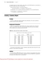
Creating a Summary Report
146
Creating a Customized Sort Order
148
Conditionally Updating a Table
150
Updating a Table with Values from Another Table
153
Creating and Using Macro Variables
154
Using PROC SQL Tables in Other SAS Procedures
157
Appendix 1
Recommended Reading 161
Recommended Reading
161
Glossary 163
Index 167
Please purchase PDF Split-Merge on www.verypdf.com to remove this watermark.
1

CHAPTER
1
Introduction to the SQL
Procedure
What Is SQL?
1
What Is the SQL Procedure?
1
Terminology 2
Tables 2
Queries
2
Views 2
Null Values
3
Comparing PROC SQL with the SAS DATA Step
3
Notes about the Example Tables
4
What Is SQL?
Structured Query Language (SQL) is a standardized, widely used language that
retrieves and updates data in relational tables and databases.
A relation is a mathematical concept that is similar to the mathematical concept of a
set. Relations are represented physically as two-dimensional tables that are arranged
in rows and columns. Relational theory was developed by E. F. Codd, an IBM
researcher, and first implemented at IBM in a prototype called System R. This
prototype evolved into commercial IBM products based on SQL. The Structured Query
Language is now in the public domain and is part of many vendors’ products.
What Is the SQL Procedure?
The SQL procedure is SAS’ implementation of Structured Query Language. PROC

SQL is part of Base SAS software, and you can use it with any SAS data set (table).
Often, PROC SQL can be an alternative to other SAS procedures or the DATA step. You
can use SAS language elements such as global statements, data set options, functions,
informats, and formats with PROC SQL just as you can with other SAS procedures.
PROC SQL can
generate reports
generate summary statistics
retrieve data from tables or views
combine data from tables or views
create tables, views, and indexes
update the data values in PROC SQL tables
update and retrieve data from database management system (DBMS) tables
Please purchase PDF Split-Merge on www.verypdf.com to remove this watermark.
2 Terminology Chapter 1
modify a PROC SQL table by adding, modifying, or dropping columns.
PROC SQL can be used in an interactive SAS session or within batch programs, and
it can include global statements, such as TITLE and OPTIONS.
Terminology
Tables
A PROC SQL table is the same as a SAS data file. It is a SAS file of type DATA.
PROC SQL tables consist of rows and columns. The rows correspond to observations in
SAS data files, and the columns correspond to variables. The following table lists
equivalent terms that are used in SQL, SAS, and traditional data processing.
SQL Term SAS Term Data Processing Term
table SAS data file file
row observation record
column variable field
You can create and modify tables by using the SAS DATA step, or by using the PROC
SQL statements that are described in Chapter 4, “Creating and Updating Tables and
Views,” on page 89. Other SAS procedures and the DATA step can read and update

tables that are created with PROC SQL.
DBMS tables are tables that were created with other software vendors’ database
management systems. PROC SQL can connect to, update, and modify DBMS tables,
with some restrictions. For more information, see “Accessing a DBMS with SAS/
ACCESS Software” on page 128.
Queries
Queries retrieve data from a table, view, or DBMS. A query returns a query result,
which consists of rows and columns from a table. With PROC SQL, you use a SELECT
statement and its subordinate clauses to form a query. Chapter 2, “Retrieving Data
from a Single Table,” on page 11 describes how to build a query.
Views
PROC SQL views do not actually contain data as tables do. Rather, a PROC SQL
view contains a stored SELECT statement or query. The query executes when you use
the view in a SAS procedure or DATA step. When a view executes, it displays data that
is derived from existing tables, from other views, or from SAS/ACCESS views. Other
SAS procedures and the DATA step can use a PROC SQL view as they would any SAS
data file. For more information about views, see Chapter 4, “Creating and Updating
Tables and Views,” on page 89.
Please purchase PDF Split-Merge on www.verypdf.com to remove this watermark.
Introduction to the SQL Procedure Comparing PROC SQL with the SAS DATA Step 3
Null Values
According to the ANSI Standard for SQL, a missing value is called a null value.Itis
not the same as a blank or zero value. However, to be compatible with the rest of SAS,
PROC SQL treats missing values the same as blanks or zero values, and considers all
three to be null values. This important concept comes up in several places in this
document.
Comparing PROC SQL with the SAS DATA Step
PROC SQL can perform some of the operations that are provided by the DATA step
and the PRINT, SORT, and SUMMARY procedures. The following query displays the
total population of all the large countries (countries with population greater than 1

million) on each continent.
proc sql;
title ’Population of Large Countries Grouped by Continent’;
select Continent, sum(Population) as TotPop format=comma15.
from sql.countries
where Population gt 1000000
group by Continent
order by TotPop;
quit;
Output 1.1 Sample SQL Output
Population of Large Countries Grouped by Continent
Continent TotPop

Oceania 3,422,548
Australia 18,255,944
Central America and Caribbean 65,283,910
South America 316,303,397
North America 384,801,818
Africa 706,611,183
Europe 811,680,062
Asia 3,379,469,458
Here is a SAS program that produces the same result.
title ’Large Countries Grouped by Continent’;
proc summary data=sql.countries;
where Population > 1000000;
class Continent;
var Population;
output out=sumPop sum=TotPop;
run;
proc sort data=SumPop;

by totPop;
run;
Please purchase PDF Split-Merge on www.verypdf.com to remove this watermark.
4 Notes about the Example Tables Chapter 1
proc print data=SumPop noobs;
var Continent TotPop;
format TotPop comma15.;
where _type_=1;
run;
Output 1.2 Sample DATA Step Output
Large Countries Grouped by Continent
Continent TotPop
Oceania 3,422,548
Australia 18,255,944
Central America and Caribbean 65,283,910
South America 316,303,397
North America 384,801,818
Africa 706,611,183
Europe 811,680,062
Asia 3,379,469,458
This example shows that PROC SQL can achieve the same results as base SAS
software but often with fewer and shorter statements. The SELECT statement that is
shown in this example performs summation, grouping, sorting, and row selection. It
also displays the query’s results without the PRINT procedure.
PROC SQL executes without using the RUN statement. After you invoke PROC SQL
you can submit additional SQL procedure statements without submitting the PROC
statement again. Use the QUIT statement to terminate the procedure.
Notes about the Example Tables
For all examples, the following global statements are in effect:
options nodate nonumber linesize=80 pagesize=60;

libname sql ’SAS-data-library’;
The tables that are used in this document contain geographic and demographic data.
The data is intended to be used for the PROC SQL code examples only; it is not
necessarily up to date or accurate.
The COUNTRIES table contains data that pertains to countries. The Area column
contains a country’s area in square miles. The UNDate column contains the year a
country entered the United Nations, if applicable.
Please purchase PDF Split-Merge on www.verypdf.com to remove this watermark.
Introduction to the SQL Procedure Notes about the Example Tables 5
Output 1.3 COUNTRIES (Partial Output)
COUNTRIES
Name Capital Population Area Continent UNDate

Afghanistan Kabul 17070323 251825 Asia 1946
Albania Tirane 3407400 11100 Europe 1955
Algeria Algiers 28171132 919595 Africa 1962
Andorra Andorra la Vell 64634 200 Europe 1993
Angola Luanda 9901050 481300 Africa 1976
Antigua and Barbuda St. John’s 65644 171 Central America 1981
Argentina Buenos Aires 34248705 1073518 South America 1945
Armenia Yerevan 3556864 11500 Asia 1992
Australia Canberra 18255944 2966200 Australia 1945
Austria Vienna 8033746 32400 Europe 1955
Azerbaijan Baku 7760064 33400 Asia 1992
Bahamas Nassau 275703 5400 Central America 1973
Bahrain Manama 591800 300 Asia 1971
Bangladesh Dhaka 1.2639E8 57300 Asia 1974
Barbados Bridgetown 258534 200 Central America 1966
The WORLDCITYCOORDS table contains latitude and longitude data for world
cities. Cities in the Western hemisphere have negative longitude coordinates. Cities in

the Southern hemisphere have negative latitude coordinates. Coordinates are rounded
to the nearest degree.
Output 1.4 WORLDCITYCOORDS (Partial Output)
WORLDCITCOORDS
City Country Latitude Longitude

Kabul Afghanistan 35 69
Algiers Algeria 37 3
Buenos Aires Argentina -34 -59
Cordoba Argentina -31 -64
Tucuman Argentina -27 -65
Adelaide Australia -35 138
Alice Springs Australia -24 134
Brisbane Australia -27 153
Darwin Australia -12 131
Melbourne Australia -38 145
Perth Australia -32 116
Sydney Australia -34 151
Vienna Austria 48 16
Nassau Bahamas 26 -77
Chittagong Bangladesh 22 92
The USCITYCOORDS table contains the coordinates for cities in the United States.
Because all cities in this table are in the Western hemisphere, all of the longitude
coordinates are negative. Coordinates are rounded to the nearest degree.
Please purchase PDF Split-Merge on www.verypdf.com to remove this watermark.
6 Notes about the Example Tables Chapter 1
Output 1.5 USCITYCOORDS (Partial Output)
USCITYCOORDS
City State Latitude Longitude

Albany NY 43 -74
Albuquerque NM 36 -106
Amarillo TX 35 -102
Anchorage AK 61 -150
Annapolis MD 39 -77
Atlanta GA 34 -84
Augusta ME 44 -70
Austin TX 30 -98
Baker OR 45 -118
Baltimore MD 39 -76
Bangor ME 45 -69
Baton Rouge LA 31 -91
Birmingham AL 33 -87
Bismarck ND 47 -101
Boise ID 43 -116
The UNITEDSTATES table contains data that is associated with the states. The
Statehood column contains the date when the state was admitted into the Union.
Output 1.6 UNITEDSTATES (Partial Output)
UNITEDSTATES
Name Capital Population Area Continent Statehood

Alabama Montgomery 4227437 52423 North America 14DEC1819
Alaska Juneau 604929 656400 North America 03JAN1959
Arizona Phoenix 3974962 114000 North America 14FEB1912
Arkansas Little Rock 2447996 53200 North America 15JUN1836
California Sacramento 31518948 163700 North America 09SEP1850
Colorado Denver 3601298 104100 North America 01AUG1876
Connecticut Hartford 3309742 5500 North America 09JAN1788
Delaware Dover 707232 2500 North America 07DEC1787
District of Colum Washington 612907 100 North America 21FEB1871

Florida Tallahassee 13814408 65800 North America 03MAR1845
Georgia Atlanta 6985572 59400 North America 02JAN1788
Hawaii Honolulu 1183198 10900 Oceania 21AUG1959
Idaho Boise 1109980 83600 North America 03JUL1890
Illinois Springfield 11813091 57900 North America 03DEC1818
Indiana Indianapolis 5769553 36400 North America 11DEC1816
The POSTALCODES table contains postal code abbreviations.
Please purchase PDF Split-Merge on www.verypdf.com to remove this watermark.
Introduction to the SQL Procedure Notes about the Example Tables 7
Output 1.7 POSTALCODES (Partial Output)
POSTALCODES
Name Code

Alabama AL
Alaska AK
American Samoa AS
Arizona AZ
Arkansas AR
California CA
Colorado CO
Connecticut CT
Delaware DE
District Of Columbia DC
Florida FL
Georgia GA
Guam GU
Hawaii HI
Idaho ID
The WORLDTEMPS table contains average high and low temperatures from various
international cities.

Output 1.8 WORLDTEMPS (Partial Output)
WORLDTEMPS
City Country AvgHigh AvgLow

Algiers Algeria 90 45
Amsterdam Netherlands 70 33
Athens Greece 89 41
Auckland New Zealand 75 44
Bangkok Thailand 95 69
Beijing China 86 17
Belgrade Yugoslavia 80 29
Berlin Germany 75 25
Bogota Colombia 69 43
Bombay India 90 68
Bucharest Romania 83 24
Budapest Hungary 80 25
Buenos Aires Argentina 87 48
Cairo Egypt 95 48
Calcutta India 97 56
The OILPROD table contains oil production statistics from oil-producing countries.
Please purchase PDF Split-Merge on www.verypdf.com to remove this watermark.
8 Notes about the Example Tables Chapter 1
Output 1.9 OILPROD (Partial Output)
OILPROD
Barrels
Country PerDay

Algeria 1,400,000
Canada 2,500,000
China 3,000,000

Egypt 900,000
Indonesia 1,500,000
Iran 4,000,000
Iraq 600,000
Kuwait 2,500,000
Libya 1,500,000
Mexico 3,400,000
Nigeria 2,000,000
Norway 3,500,000
Oman 900,000
Saudi Arabia 9,000,000
United States of America 8,000,000
The OILRSRVS table lists approximate oil reserves of oil-producing countries.
Output 1.10 OILRSRVS (Partial Output)
OILRSRVS
Country Barrels

Algeria 9,200,000,000
Canada 7,000,000,000
China 25,000,000,000
Egypt 4,000,000,000
Gabon 1,000,000,000
Indonesia 5,000,000,000
Iran 90,000,000,000
Iraq 110,000,000,000
Kuwait 95,000,000,000
Libya 30,000,000,000
Mexico 50,000,000,000
Nigeria 16,000,000,000
Norway 11,000,000,000

Saudi Arabia 260,000,000,000
United Arab Emirates 100,000,000
The CONTINENTS table contains geographic data that relates to world continents.
Please purchase PDF Split-Merge on www.verypdf.com to remove this watermark.
Introduction to the SQL Procedure Notes about the Example Tables 9
Output 1.11 CONTINENTS
CONTINENTS
Name Area HighPoint Height LowPoint Depth

Africa 11506000 Kilimanjaro 19340 Lake Assal -512
Antarctica 5500000 Vinson Massif 16860 .
Asia 16988000 Everest 29028 Dead Sea -1302
Australia 2968000 Kosciusko 7310 Lake Eyre -52
Central America . . .
Europe 3745000 El’brus 18510 Caspian Sea -92
North America 9390000 McKinley 20320 Death Valley -282
Oceania . . .
South America 6795000 Aconcagua 22834 Valdes Peninsul -131
The FEATURES table contains statistics that describe various types of geographical
features, such as oceans, lakes, and mountains.
Output 1.12 FEATURES (Partial Output)
FEATURES
Name Type Location Area Height Depth Length

Aconcagua Mountain Argentina . 22834 . .
Amazon River South America . . . 4000
Amur River Asia . . . 2700
Andaman Sea 218100 . 3667 .
Angel Falls Waterfall Venezuela . 3212 . .
Annapurna Mountain Nepal . 26504 . .

Aral Sea Lake Asia 25300 . 222 .
Ararat Mountain Turkey . 16804 . .
Arctic Ocean 5105700 . 17880 .
Atlantic Ocean 33420000 . 28374 .
Baffin Island Arctic 183810 . . .
Baltic Sea 146500 . 180 .
Baykal Lake Russia 11780 . 5315 .
Bering Sea 873000 . 4893 .
Black Sea 196100 . 3906 .
Please purchase PDF Split-Merge on www.verypdf.com to remove this watermark.
10
Please purchase PDF Split-Merge on www.verypdf.com to remove this watermark.
11
CHAPTER
2
Retrieving Data from a Single
Table
Overview of the SELECT Statement
12
SELECT and FROM Clauses
12
WHERE Clause
13
ORDER BY Clause
13
GROUP BY Clause
13
HAVING Clause 13
Ordering the SELECT Statement
14

Selecting Columns in a Table
14
Selecting All Columns in a Table
14
Selecting Specific Columns in a Table
15
Eliminating Duplicate Rows from the Query Results
16
Determining the Structure of a Table
17
Creating New Columns 18
Adding Text to Output 18
Calculating Values 19
Assigning a Column Alias 20
Referring to a Calculated Column by Alias 21
Assigning Values Conditionally 21
Using a Simple CASE Expression 22
Using the CASE-OPERAND Form 23
Replacing Missing Values 24
Specifying Column Attributes 24
Sorting Data 25
Sorting by Column 25
Sorting by Multiple Columns 26
Specifying a Sort Order 27
Sorting by Calculated Column 27
Sorting by Column Position 28
Sorting by Unselected Columns 29
Specifying a Different Sorting Sequence 29
Sorting Columns That Contain Missing Values 30
Retrieving Rows That Satisfy a Condition 30

Using a Simple WHERE Clause 30
Retrieving Rows Based on a Comparison 31
Retrieving Rows That Satisfy Multiple Conditions 32
Using Other Conditional Operators 33
Using the IN Operator 34
Using the IS MISSING Operator 34
Using the BETWEEN-AND Operators 35
Using the LIKE Operator 36
Using Truncated String Comparison Operators 37
Please purchase PDF Split-Merge on www.verypdf.com to remove this watermark.
12 Overview of the SELECT Statement Chapter 2
Using a WHERE Clause with Missing Values
37
Summarizing Data
39
Using Aggregate Functions
39
Summarizing Data with a WHERE Clause
40
Using the MEAN Function with a WHERE Clause
40
Displaying Sums
40
Combining Data from Multiple Rows into a Single Row
41
Remerging Summary Statistics
41
Using Aggregate Functions with Unique Values
43
Counting Unique Values

43
Counting Nonmissing Values
43
Counting All Rows
44
Summarizing Data with Missing Values
44
Finding Errors Caused by Missing Values
44
Grouping Data
45
Grouping by One Column
46
Grouping without Summarizing
46
Grouping by Multiple Columns
47
Grouping and Sorting Data
48
Grouping with Missing Values
48
Finding Grouping Errors Caused by Missing Values
49
Filtering Grouped Data
50
Using a Simple HAVING Clause
50
Choosing Between HAVING and WHERE
51
Using HAVING with Aggregate Functions

51
Validating a Query
52
Overview of the SELECT Statement
This chapter shows you how to
retrieve data from a single table by using the SELECT statement
validate the correctness of a SELECT statement by using the VALIDATE
statement.
With the SELECT statement, you can retrieve data from tables or data that is
described by SAS data views.
Note: The examples in this chapter retrieve data from tables that are SAS data
sets. However, you can use all of the operations that are described here with SAS data
views.
The SELECT statement is the primary tool of PROC SQL. You use it to identify,
retrieve, and manipulate columns of data from a table. You can also use several
optional clauses within the SELECT statement to place restrictions on a query.
SELECT and FROM Clauses
The following simple SELECT statement is sufficient to produce a useful result:
select Name
from sql.countries;
The SELECT statement must contain a SELECT clause and a FROM clause, both of
which are required in a PROC SQL query. This SELECT statement contains
Please purchase PDF Split-Merge on www.verypdf.com to remove this watermark.
Retrieving Data from a Single Table Overview of the SELECT Statement 13
a SELECT clause that lists the Name column
a FROM clause that lists the table in which the Name column resides.
WHERE Clause
The WHERE clause enables you to restrict the data that you retrieve by specifying a
condition that each row of the table must satisfy. PROC SQL output includes only those
rows that satisfy the condition. The following SELECT statement contains a WHERE

clause that restricts the query output to only those countries that have a population
that is greater than 5,000,000 people:
select Name
from sql.countries
where Population gt 5000000;
ORDER BY Clause
The ORDER BY clause enables you to sort the output from a table by one or more
columns; that is, you can put character values in either ascending or descending
alphabetical order, and you can put numerical values in either ascending or descending
numerical order. The default order is ascending. For example, you can modify the
previous example to list the data by descending population:
select Name
from sql.countries
where Population gt 5000000
order by Population desc;
GROUP BY Clause
The GROUP BY clause enables you to break query results into subsets of rows.
When you use the GROUP BY clause, you use an aggregate function in the SELECT
clause or a HAVING clause to instruct PROC SQL how to group the data. For details
about aggregate functions, see “Summarizing Data” on page 39. PROC SQL calculates
the aggregate function separately for each group. When you do not use an aggregate
function, PROC SQL treats the GROUP BY clause as if it were an ORDER BY clause,
and any aggregate functions are applied to the entire table.
The following query uses the SUM function to list the total population of each
continent. The GROUP BY clause groups the countries by continent, and the ORDER
BY clause puts the continents in alphabetical order:
select Continent, sum(Population)
from sql.countries
group by Continent
order by Continent;

HAVING Clause
The HAVING clause works with the GROUP BY clause to restrict the groups in a
query’s results based on a given condition. PROC SQL applies the HAVING condition
after grouping the data and applying aggregate functions. For example, the following
query restricts the groups to include only the continents of Asia and Europe:
select Continent, sum(Population)
from sql.countries
group by Continent
Please purchase PDF Split-Merge on www.verypdf.com to remove this watermark.
14 Selecting Columns in a Table Chapter 2
having Continent in (’Asia’, ’Europe’)
order by Continent;
Ordering the SELECT Statement
When you construct a SELECT statement, you must specify the clauses in the
following order:
1
SELECT
2
FROM
3
WHERE
4 GROUP BY
5
HAVING
6
ORDER BY
Note: Only the SELECT and FROM clauses are required.
The PROC SQL SELECT statement and its clauses are discussed in further detail in
the following sections.
Selecting Columns in a Table

When you retrieve data from a table, you can select one or more columns by using
variations of the basic SELECT statement.
Selecting All Columns in a Table
Use an asterisk in the SELECT clause to select all columns in a table. The following
example selects all columns in the SQL.USCITYCOORDS table, which contains latitude
and longitude values for U.S. cities:
proc sql outobs=12;
title ’U.S. Cities with Their States and Coordinates’;
select *
from sql.uscitycoords;
Note: The OUTOBS= option limits the number of rows (observations) in the output.
OUTOBS= is similar to the OBS= data set option. OUTOBS= is used throughout this
document to limit the number of rows that are displayed in examples.
Note: In the tables used in these examples, latitude values that are south of the
Equator are negative. Longitude values that are west of the Prime Meridian are also
negative.
Please purchase PDF Split-Merge on www.verypdf.com to remove this watermark.
Retrieving Data from a Single Table Selecting Specific Columns in a Table 15
Output 2.1 Selecting All Columns in a Table
U.S. Cities with Their States and Coordinates
City State Latitude Longitude

Albany NY 43 -74
Albuquerque NM 36 -106
Amarillo TX 35 -102
Anchorage AK 61 -150
Annapolis MD 39 -77
Atlanta GA 34 -84
Augusta ME 44 -70
Austin TX 30 -98

Baker OR 45 -118
Baltimore MD 39 -76
Bangor ME 45 -69
Baton Rouge LA 31 -91
Note: When you select all columns, PROC SQL displays the columns in the order in
which they are stored in the table.
Selecting Specific Columns in a Table
To select a specific column in a table, list the name of the column in the SELECT
clause. The following example selects only the City column in the
SQL.USCITYCOORDS table:
proc sql outobs=12;
title ’Names of U.S. Cities’;
select City
from sql.uscitycoords;
Output 2.2 Selecting One Column
Names of U.S. Cities
City

Albany
Albuquerque
Amarillo
Anchorage
Annapolis
Atlanta
Augusta
Austin
Baker
Baltimore
Bangor
Baton Rouge

Please purchase PDF Split-Merge on www.verypdf.com to remove this watermark.
16 Eliminating Duplicate Rows from the Query Results Chapter 2
If you want to select more than one column, then you must separate the names of the
columns with commas, as in this example, which selects the City and State columns in
the SQL.USCITYCOORDS table:
proc sql outobs=12;
title ’U.S. Cities and Their States’;
select City, State
from sql.uscitycoords;
Output 2.3 Selecting Multiple Columns
U.S. Cities and Their States
City State

Albany NY
Albuquerque NM
Amarillo TX
Anchorage AK
Annapolis MD
Atlanta GA
Augusta ME
Austin TX
Baker OR
Baltimore MD
Bangor ME
Baton Rouge LA
Note: When you select specific columns, PROC SQL displays the columns in the
order in which you specify them in the SELECT clause.
Eliminating Duplicate Rows from the Query Results
In some cases, you might want to find only the unique values in a column. For
example, if you want to find the unique continents in which U.S. states are located,

then you might begin by constructing the following query:
proc sql outobs=12;
title ’Continents of the United States’;
select Continent
from sql.unitedstates;
Please purchase PDF Split-Merge on www.verypdf.com to remove this watermark.
Retrieving Data from a Single Table Determining the Structure of a Table 17
Output 2.4 Selecting a Column with Duplicate Values
Continents of the United States
Continent

North America
North America
North America
North America
North America
North America
North America
North America
North America
North America
North America
Oceania
You can eliminate the duplicate rows from the results by using the DISTINCT
keyword in the SELECT clause. Compare the previous example with the following
query, which uses the DISTINCT keyword to produce a single row of output for each
continent that is in the SQL.UNITEDSTATES table:
proc sql;
title ’Continents of the United States’;
select distinct Continent

from sql.unitedstates;
Output 2.5 Eliminating Duplicate Values
Continents of the United States
Continent

North America
Oceania
Note: When you specify all of a table’s columns in a SELECT clause with the
DISTINCT keyword, PROC SQL eliminates duplicate rows, or rows in which the values
in all of the columns match, from the results.
Determining the Structure of a Table
To obtain a list of all of the columns in a table and their attributes, you can use the
DESCRIBE TABLE statement. The following example generates a description of the
SQL.UNITEDSTATES table. PROC SQL writes the description to the log.
proc sql;
describe table sql.unitedstates;
Please purchase PDF Split-Merge on www.verypdf.com to remove this watermark.
18 Creating New Columns Chapter 2
Output 2.6 Determining the Structure of a Table (Partial Log)
NOTE: SQL table SQL.UNITEDSTATES was created like:
create table SQL.UNITEDSTATES( bufsize=12288 )
(
Name char(35) format=$35. informat=$35. label=’Name’,
Capital char(35) format=$35. informat=$35. label=’Capital’,
Population num format=BEST8. informat=BEST8. label=’Population’,
Area num format=BEST8. informat=BEST8.,
Continent char(35) format=$35. informat=$35. label=’Continent’,
Statehood num
);
Creating New Columns

In addition to selecting columns that are stored in a table, you can create new
columns that exist for the duration of the query. These columns can contain text or
calculations. PROC SQL writes the columns that you create as if they were columns
from the table.
Adding Text to Output
You can add text to the output by including a string expression, or literal expression,
in a query. The following query includes two strings as additional columns in the output:
proc sql outobs=12;
title ’U.S. Postal Codes’;
select ’Postal code for’, Name, ’is’, Code
from sql.postalcodes;
Output 2.7 Adding Text to Output
U.S. Postal Codes
Name Code

Postal code for Alabama is AL
Postal code for Alaska is AK
Postal code for American Samoa is AS
Postal code for Arizona is AZ
Postal code for Arkansas is AR
Postal code for California is CA
Postal code for Colorado is CO
Postal code for Connecticut is CT
Postal code for Delaware is DE
Postal code for District Of Columbia is DC
Postal code for Florida is FL
Postal code for Georgia is GA
Please purchase PDF Split-Merge on www.verypdf.com to remove this watermark.
Retrieving Data from a Single Table Calculating Values 19
To prevent the column headers Name and Code from printing, you can assign a label

that starts with a special character to each of the columns. PROC SQL does not output
the column name when a label is assigned, and it does not output labels that begin with
special characters. For example, you could use the following query to suppress the
column headers that PROC SQL displayed in the previous example:
proc sql outobs=12;
title ’U.S. Postal Codes’;
select ’Postal code for’, Name label=’#’, ’is’, Code label=’#’
from sql.postalcodes;
Output 2.8 Suppressing Column Headers in Output
U.S. Postal Codes

Postal code for Alabama is AL
Postal code for Alaska is AK
Postal code for American Samoa is AS
Postal code for Arizona is AZ
Postal code for Arkansas is AR
Postal code for California is CA
Postal code for Colorado is CO
Postal code for Connecticut is CT
Postal code for Delaware is DE
Postal code for District Of Columbia is DC
Postal code for Florida is FL
Postal code for Georgia is GA
Calculating Values
You can perform calculations with values that you retrieve from numeric columns.
The following example converts temperatures in the SQL.WORLDTEMPS table from
Fahrenheit to Celsius:
proc sql outobs=12;
title ’Low Temperatures in Celsius’;
select City, (AvgLow - 32) * 5/9 format=4.1

from sql.worldtemps;
Note: This example uses the FORMAT attribute to modify the format of the
calculated output. See “Specifying Column Attributes” on page 24 for more
information.
Please purchase PDF Split-Merge on www.verypdf.com to remove this watermark.
20 Assigning a Column Alias Chapter 2
Output 2.9 Calculating Values
Low Temperatures in Celsius
City

Algiers 7.2
Amsterdam 0.6
Athens 5.0
Auckland 6.7
Bangkok 20.6
Beijing -8.3
Belgrade -1.7
Berlin -3.9
Bogota 6.1
Bombay 20.0
Bucharest -4.4
Budapest -3.9
Assigning a Column Alias
By specifying a column alias, you can assign a new name to any column within a
PROC SQL query. The new name must follow the rules for SAS names. The name
persists only for that query.
When you use an alias to name a column, you can use the alias to reference the
column later in the query. PROC SQL uses the alias as the column heading in output.
The following example assigns an alias of LowCelsius to the calculated column from the
previous example:

proc sql outobs=12;
title ’Low Temperatures in Celsius’;
select City, (AvgLow - 32) * 5/9 as LowCelsius format=4.1
from sql.worldtemps;
Output 2.10 Assigning a Column Alias to a Calculated Column
Low Temperatures in Celsius
City LowCelsius

Algiers 7.2
Amsterdam 0.6
Athens 5.0
Auckland 6.7
Bangkok 20.6
Beijing -8.3
Belgrade -1.7
Berlin -3.9
Bogota 6.1
Bombay 20.0
Bucharest -4.4
Budapest -3.9
Please purchase PDF Split-Merge on www.verypdf.com to remove this watermark.