Tài liệu Database Systems: The Complete Book- P13 docx

tells us that total sales of all Aardvark lnodels in all colors, over all time at all
dealers is 198.000 cars for
a
total price of $3,521,727,000.
Consider how to answer
a
query in \\-hich we specify conditions on certain
attributes of the Sales relation and group by
some other attributes, n-hile
asking for the sum, count, or average price. In the relation
are r sales),
we
look for those tuples
t
with the fo1lov;ing properties:
1. If the query specifies
a
value
v
for attribute
a;
then tuple
t
has
v
in its
component for
a.
2. If the query groups by an attribute
a,
then

t
has any non-* value in its
conlponent for
a.
3.
If the query neither groups by attribute
a
nor specifies a value for
a.
then
t
has
*
in its component for
a.
Each tuple
t
has tlie sum and count for one of the desired groups. If n-e \%-ant
the average price, a division is performed on the sum and count conlponents of
each tuple
t.
Example
20.18
:
The query
SELECT color,
AVG(price)
FROM Sales
WHERE model
=

'Gobi'
GROUP
BY
color;
is ansn-ered by looking for all tuples of
sales)
~vith the form
('Gobi',
C.
*,
*,
21,
n)
here
c
is any specific color. In this tuple,
v
will be the sum of sales of Gobis
in that color, while
n
will be the nlini!)cr of sales of Gobis in that color. Tlie
average price. although not an attribute of Sales or
sales)
directly. is
v/n.
Tlie answer to the query is the set of
(c,
vln)
pairs obtained fi-om all
('Gobi'.

c,
*,
*.
v.
n)
tuples.
20.5.2
Cube ImplementaOion
by
Materialized Views
11%
suggested in Fig. 20.17 that adding
aggregations
to the cube doesn't cost
much in tcrms of space. and saves a lot in time \vhen the common kincis of
decision-support queries are asked.
Ho~vever: our analysis is based on the as-
sumption that queries choose either to aggregate completely in a dimension
or not to aggregate at all. For some
dime~isions. there are many degrees of
granularity that could be chosen for a grouping on
that dimension.
Uc have already mentioned thc case of time. xvl-here numerolls options such
as aggregation by
weeks, months: quarters, or ycars exist,, in addition to the
all-or-nothing choices of grouping by day or aggregating over all time. For
another esanlple based on our running automobile database, Ive could choose
to aggregate dealers completely or not aggregate them at all.
Hon-ever, we could
also choose to aggregate by city, by state, or perhaps by other regions, larger

or smaller. Thus: there are at least
sis choices of grouping for time and at least
four for dealers.
l\Tllen the number of choices for grouping along each dimension grows, it
becomes increasingly expensive to store the results of aggregating by every
possible
conlbination of groupings. Sot only are there too many of them, but
they are not as easily organized as
the structure of Fig. 20.17 suggests for tlle
all-or-nothing case. Thus, commercial data-cube systems may help the user to
choose
some
n~aterialized
views
of the data cube.
A
materialized view is the
result of some query,
which we choose to store in the database, rather than
reconstructing (parts of) it as needed in response to queries. For the data cube,
the vie~vs we n-ould choose to materialize xi11 typically be aggregations of the
full data cube.
The coarser the partition implied by the grouping, the less space the mate-
rialized
view takes. On the other hand, if ire ~vant to use a view to answer a
certain query,
then the view must not partition any dimension more coarsely
than the query does. Thus, to
maximize the utility of materialized views, we
generally n-ant some large \-iers that group dimensions into a fairly fine parti-

tion. In addition, the choice of
vien-s to materialize is heavily influenced by the
kinds of
queries that the analysts are likely
to
ask.
.in
example will suggest tlie
tradeoffs in\-011-ed.
INSERT INTO SalesVl
SELECT model, color, month, city,
SUM(va1) AS val, SUM(cnt) AS cnt
FROM Sales JOIN Dealers
ON
dealer
=
name
GROUP
BY
model, color, month, city;
Figure 20.18: The materialized
vien. SalesVl
Example
20.19
:
Let us return to the data cube
Sales (model, color, date, dealer,
val
,
cnt)

that ne de\-eloped in Esample 20.17. One possible materialized vie\\- groups
dates by
nionth and dealers by city. This view. 1%-hich
1%-e
call SalesV1, is
constlucted
by
the query in Fig. 20.18. This query is not strict
SQL.
since n-e
imagine that dates and their grouping units such as months are understood
by the data-cube system n-ithout being told to join Sales with the imaginary
relation
rep~esenting dajs that \ve discussed in Example 20.14.
CHAPTER
20.
IiYFORI\IATIOAr IArTEGR.4TION
20.5.
DdT.4 CUBES
1055
INSERT INTO SalesV2
SELECT model, week, state,
SUM(va1) AS val, SUM(cnt) AS cnt
FROM Sales
JOIN Dealers
ON
dealer
=
name
GROUP

BY
model, week, state;
Figure 20.19: Another materialized view,
SalesV2
Another possible materialized view aggregates colors completely, aggregates
time into
u-eeks, and dealers by states. This view,
SalesV2,
is defined by the
query in Fig. 20.19. Either view
SalesVl
or
SalesV2
can be used to ansn-er a
query that partitions no more finely than either in any dimension. Thus, the
query
41:
SELECT model, SUM(va1)
FROM Sales
GROUP
BY
model;
can be answered either by
SELECT model, SUM(va1)
FROM SalesVl
GROUP
BY
model;
SELECT model,
SUM(va1)

FROM SalesV2
GROUP BY model;
On the other hand, the query
42: SELECT model, year, state, SUM(va1)
FROM Sales JOIN Dealers
ON
dealer
=
name
GROUP
BY
model, year, state;
can on1 be ans\vered from
SalesV1.
as
SELECT model, year, state, SUM(va1)
FROM SalesVl
GROUP
BY
model, year, state;
Incidentally. the query inmediately above. like the qu'rics that nggregate time
units, is not strict
SQL.
That is.
state
is not ari attribute of
SalesVl:
only
city
is. \Ye rmust assume that the data-cube systenl knol\-s how to perform the

aggregation of cities into states, probably by accessing the dimension table for
dealers.
\Ye
cannot answer Q2 from
SalesV2.
Although we could roll-up cities into
states
(i.e aggregate the cities into their states) to use
SalesV1,
we
carrrlot
roll-up ~veeks into years, since years are not evenly divided into weeks. and
data from a
week beginning. say, Dec.
29,
2001. contributes to years 2001 and
2002 in a way we
carinot tell from the data aggregated by weeks.
Finally, a query like
43:
SELECT model, color, date, ~~~(val)
FROM Sales
GROUP BY model, color, date;
can be anslvered from neither
SalesVl
nor
SalesV2.
It cannot be answered
from
Salesvl

because its partition of days by ~nonths is too coarse to recover
sales by day,
and it cannot be ans~vered from
SalesV2
because that view does
not group by color. We would have to answer this query directly from the full
data cube.
20.5.3
The Lattice
of
Views
To formalize the cbservations of Example 20.10. it he!ps to think of a lattice of
possibl~ groupings for each dimension of the cube. The points of the lattice are
the
ways that we can partition the ~alucs of a dimension
by
grouping according
to one or
more attributes of its dimension table.
nB
say that partition
PI
is
belo~v partition
P2.
written
PI
5
P2
if and only if each group of

Pl
is contained
within some group of
PZ.
All
Years
/
1
I
Quarters
I
Weeks Months
Days
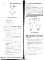
Figure 20.20:
A
lattice of partitions for time inter\-als
Example
20.20:
For the lattice of time partitions n-e might choose the dia-
gram of Fig. 20.20.
-4
path from some node
fi
dotvn to
PI
means that
PI
5
4.
These are not the only possible units of time, but they

\\-ill
serve as an example
of what units a s~stern might support. Sotice that daks lie below both \reeks
and months, but weeks do not lie below months. The reason is that while a
group of events that took place in
one day surely took place within one \reek
and within one month. it is not true that a group of events taking place in one
week necessarily took place in any one month. Similarly, a week's group need
not be contained within the group
cor~esponding to one quarter or to one year.
At
tlie top is a partition we call "all," meaning that events are grouped into a
single group;
i.e we niake no distinctions among diffeient times.
All
I
State
I
City
I
Dealer
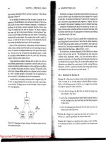
Figure 20.21:
A
lattice of partitions for automobile dealers
Figure 20.21
shows another lattice, this time for the dealer dimension of our
automobiles example. This lattice is siniplcr: it shows that partitioning sales
by
dealer gives a finer partition than partitioning by the city of the dealer. i<-hich is
in turn finer than partitioning by tlie state of tlie dealer.

The top of tlle ldrtice
is the partition that places all dealers in one group.
Having a lattice for each dimension,
15-12
can now define a lattice for all the
possible materialized
views of a data cube that can be formed by grouping
according to some partition
in each dimension. If
15
and
1%
are two views
formed by choosing a partition (grouping) for
each dimension, then
1;
5
11
means that in each dimension, the partition
Pl
that ~ve use in
1;
is at least as
fine as the partition
Pl
that n.e use for that dimension in
Ti;
that is.
Pl
5

P?
Man) OLAP queries can also be placed in the lattice of views
In
fact. fie-
quently an OLAP query has the same form as the views we have described: the
query specifies some pa~titioning (possibly none or all) for each of the dimen-
sions. Other
OL.iP queiics involve tliis same soit of grouping, and then "slice
tlie cube to
focus
011
a subset of the data. as nas suggested
by
the diag~ani in
Fig. 20.15.
The general rule is.
I\c can ansn-er a quciy
Q
using view
1-
if and o~ily if
1-
5
Q.
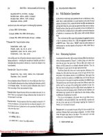
Example 20.21
:
Figure 20.22 takes the vielvs and queries of Example 20.19
and places them in a lattice.
Sotice that the Sales data cube itself is technically
a view. corresponding to tlie finest possible partition along each climensio~l. As

we observed in the original example,
QI
can be ans~vered from either SalesVl or
Sales
Figure 20.22: The lattice of
views and queries from Example 20.19
SalesV2; of course it could also be answered froni the full data cube Sales, but
there is
no reason to want to do so if one of the other views is materialized.
Q2
can be answered from either SalesVl or Sales, while
Q3
can only be answered
from Sales. Each of these relationships is expressed in Fig. 20.22 by the paths
downxard from the queries to their supporting vie~vs.
Placing queries in the lattice of views helps design data-cube databases.
Some recently developed design tools for data-cube
systems start with a set of
queries that they regard as
typical" of the application at hand. They then
select
a
set of views to materialize so that each of these queries is above at least
one of the
riel\-s, preferably identical to it or very close (i.e., the query and the
view use the same grouping in most of the dimensions).
20.5.4
Exercises
for
Section

20.5
Exercise 20.5.1
:
IVhat is the ratio of the size of CCBE(F) to the size of
F
if
fact table
F
has the follorving characteristics?
*
a)
F
has ten dimension attributes, each with ten different values.
b)
F
has ten dimension attributes. each with two differcnt values.
Exercise 20.5.2:
Let us use the cube ~nBE(Sa1es) from Example 20.17,
~vhich was built from the relation
Sales (model, color, date, dealer,
val,
cnt)
Tcll I\-hat tuples of the cube n-e 15-ould use to answer tlle follon-ing queries:
*
a) Find the total sales of I~lue cars for each dealer.
b) Find the total
nurnber of green Gobis sold by dealer .'Smilin' Sally."
c) Find the average number of
Gobis sold on each day of March, 2002 by
each dealer.

1088
CHAPTER
20.
ISFORJlATIOS IXTEGRA4TIOS
*!
Exercise
20.5.3:
In Exercise 20.4.1 lve spoke of PC-order data organized as
a cube. If we are to apply the
CCBE operator, we might find it convenient to
break several dimensions more finely. For example, instead of one processor
dimension,
we might have one dimension for the type (e.g., AlID Duron or
Pentium-IV), and another
d~mension for the speed. Suggest a set of dimrnsions
and dependent attributes that will allow us to obtain answers to a variety of
useful aggregation queries. In particular,
what role does the customer play?
.Also, the price in Exercise 20.4.1 referred to the price of one macll~ne, while
several identical machines could be ordered in a single tuple.
What should the
dependent
attribute(s) be?
Exercise
20.5.4
:
What tuples of the cube from Exercise 20.5.3 would you use
to answer the following queries?
a) Find, for each processor speed, the total number of computers ordered in
each month of the year 2002.

b) List for
each type of hard disk (e.g., SCSI or IDE) and eacli processor
type
the number of computers ordered.
c) Find the average price of computers with
1500 megahertz processors for
each month from Jan., 2001.
!
Exercise
20.5.5
:
The computers described in the cube of Exercise 20.5.3 do
not include monitors.
IVhat dimensions would you suggest to represent moni-
tors? You
may assume that the price of the monitor is included in the price of
the computer.
Exercise
20.5.6
:
Suppose that a cube has 10 dimensions. and eacli dimension
has
5
options for granularity of aggregation. including "no aggregation" and
"aggregate fully.''
How many different views can we construct by clioosing a
granularity in each
dinlension?
Exercise
20.5.7

:
Show how to add the following time units to the lattice of
Fig. 20.20: hours, minutes, seconds, fortnights
(two-week periods). decades.
and centuries.
Exercise
20.5.8:
How 15-onld you change the dealer lattice of Fig. 20.21 to
include
-regions." ~f:
a)
A
region is a set of states.
*
b) Regions are not com~liensurate with states. but each city is in only one
region.
c) Regions are like area codes: each region is contained
\vithin a state. some
cities are in
two or more regions. and some regions ha~e several cities.
20.6.
DATA
-111-YIA-G
1089
!
Exercise
20.5.9:
In Exercise 20.5.3 ne designed a cube suitable for use ~vith
the CCBE operator.
Horn-ever.

some of the dimensions could also be given a non-
trivial lattice structure. In particular, the processor type could be organized by
manufacturer (e
g., SUT, Intel. .AND. llotorola). series (e.g
SUN
Ult~aSparc.
Intel Pentium or Celeron. AlID rlthlon, or llotorola G-series), and model (e.g.,
Pentiuni-I\- or G4).
a) Design tlie lattice of processor types following the examples described
above.
b) Define a view that groups processors by series, hard disks by type, and
removable disks by speed, aggregating everything else.
c) Define a
view that groups processors by manufacturer, hard disks by
speed. and aggregates everything else except memory size.
d) Give esamples of
qneries that can be ansn-ered from the view of (11) only,
the
vieiv of (c) only, both, and neither.
*!!
Exercise
20.5.10:
If the fact table
F
to n-hicli n-e apply the
CuBE
operator is
sparse
(i.e there are inany fen-er tuples in
F

than the product of the number
of possihle values along each dimension), then tlie ratio of the sizes of CCBE(F)
and
F
can be very large. Hon large can it be?
20.6
Data
Mining
A
family of database applications cal!ed
data
rnin,ing
or
knowledge discovery
in
dntnbases
has captured considerable interest because of opportunities to learn
surprising facts
fro111 esisting databases. Data-mining queries can be thought
of as an estended
form of decision-support querx, although the distinction is in-
formal (see the
box on -Data-llining Queries and Decision-Support Queries").
Data
nli11i11:. stresses both the cpcry-optimization and data-management com-
ponents of a traditional database system, as
1%-ell as suggesting some important
estensions to database languages, such as language
primitix-es that support effi-
cient sampling of data. In

this section, we shall esamine the principal directions
data-mining applications have taken.
Me then focus on tlie problem called "fre-
quc'iit iteinsets." n-hich has 1-eceiwd the most attention from the database point
of
view.
20.6.1
Data-Iblining Applications
Broadly. data-mining queries ask for a useful summary of data, often ~vithout
suggcstir~g the values of para~netcrs that would best yield such a summary.
This family of problems thus requires rethinking the nay database systems are
to be used to provide
snch insights abo~it the data. Below are some of tlie
applications
and problems that are being addressed using very large amounts
1092
CHAPTER
20.
I;YFORhlATION INTEGR.4TION
(stop words)
such as .'and" or 'The." which tend to be present in all docu-
ments and tell us nothing about the content
A
document is placed in this
space according to the fraction of its word occurrences that are any particular
word. For instance, if the document has
1000 word occurrences, two of which
are "database." then the doculllent ~vould be placed at the ,002 coordinate in
the dimension

cor~esponding to "database." By clustering documents in this
space, we tend to get groups of documents that talk about the same thing.
For instance, documents that talk about databases might
have occurrences of
words like "data," "query," "lock,"
and so on, while documents about baseball
are unlikely to
have occurrences of these rvords.
The data-mining problem here is to take the data and select the
"means"
or centers of the clusters. Often the number of clusters is given in advance.
although that number niay be selectable by the data-mining process as
ti-ell.
Either way, a naive algorithm for choosing the centers so that the average
distance from a point to its nearest center is minimized involves many queries;
each of which does a complex aggregation.
20.6.2
Finding
Frequent Sets
of
Items
Now. we shall see a data-mining problem for which algorithms using secondary
storage effectively have been developed. The problem is most easily described
in terms of its principal application: the analysis of
market-basket
data. Stores
today often hold in a data warehouse a record of what customers have bought
together. That is,
a
customer approaches the checkout with a .'market basket"

full of the items he or she has selected. The cash register records all of these
items as part of
a
single transaction. Thus, even if lve don't know anything
about the customer, and
we
can't tell if the customer returns and buys addi-
tional items.
we
do
know certain items that a single customer bu-s together.
If items appear together in market baskets more often
than ~vould be es-
pected, then the store has an opportunity to learn something about how cus-
tomers are likely to traverse the store. The items can
be placed in the store so
that customers
will tend to take certain paths through the store, and attractive
items can be placed along these paths.
Example
20.22
:
.A
famous example. which has been clainied by several peo-
ple; is
the discovery that people rvho buy diapcrs are unusually likely also to
buy beer. Theories have
been advanced foi n.hy that relationship is true. in-
cluding
tile possibility that peoplc n-110 buy diapers. having a baby at home. ale

less likely to go out to a bar in the evening and therefore tcnd to drink beer at
home. Stores may use the fact that
inany customers 15-ill walk through the store
from where the diapers are to where the
beer is. or vice versa. Clever maiketers
place beer and diapers near each other, rvitli potato chips in the middle. The
claim is that sales of all three items then increase.
We can represent market-basket data by a fact table:
Baskets (basket, item)
where the first attribute is a .'basket ID," or unique identifier for a market
basket, and the
secoild attribute is the ID of some item found in that basket.
Sote that it is not essential for the relation to come from true ma~ket-basket
data; it could be any relation from which we xant to find associated items. For
~nstance, the '.baskets" could be documents and the "items" could be words,
in which case
ne are really looking for words that appear in many documents
together.
The simplest form of market-basket analysis searches for sets of items that
frequently appear together in market baskets. The
support
for a set of items is
the number of baskets in
which all those items appear. The problem of finding
frequent sets of ~tems
is to find, given a support threshold
s,
all those sets of
items that have support at least
s.

If the number of items in the database is large, then even if we restrict our
attention to small sets, say pairs of items only, the
time needed to count the
support for all pairs of items is enormous. Thus, the straightforward way to
solve even the frequent pairs problem
-
compute the support for each pair of
items
z
and
j,
as suggested by the SQL query in Fig. 20.24
-
~vill not work
This query involves joining
Baskets
r~ith itself, grouping the resulting tuples
by the
tri-o lte~ns found
111
that tuple, and throwing anay groups where the
number of baskets is belon- the support threshold
s
Sote that the condition
I. item
<
J. item
in the WHERE-clause is there to prevent the same pair from
being considered in
both orders. or for a .'pair" consisting of the same item

twice from being considered at all.
SELECT
I.itern, J.item, COUNT(I.basket)
FROM Baskets I, Baskets
J
WHERE 1.basket
=
J.basket AND
I.item
<
J.item
GROUP BY I.item, J.item
HAVING COUNT(I.basket)
>=
s;
Figure 20.24: Saive way to find all high-support pairs of items
20.6.3
The A-Priori Algorithm
There is an optimization that greatly reduccs the running time of a qutry like
Fig. 20.21
\\-hen the support threshold is sufficiently large that few pairs meet
it. It is ieaso~iable to set the threshold high, because a list of thousands or
millions of pairs
would not be very useful anyxay; ri-e xi-ant the data-mining
query to focus our attention on a
sn~all number of the best candidates. The
a-przorz
algorithm is based on the folloiving observation:
1094
CHAPTER

20.
IATFORlI~4TION INTEGR.ATION
Association
Rules
A
more complex type of market-basket mining searches for
associatzon
~xles
of the form {il, 22,
.
.
.
,
in)
3
j.
TKO possible properties that \ve
might want in useful rules of this form are:
1.
Confidence:
the probability of finding item
j
in a basket that has
all of
{il,i2
. .
,
in) is above a certain threshold. e.g., 50%; e.g "at
least 50% of the people who buy diapers buy beer."
2.

Interest:
the probability of finding item
j
in a basket that has all
of
{il,
i2,.
. .
,in} is significantly higher or lower than the probability
of finding
j
in a random basket.
In
statistical terms,
j
correlates
with
{il,
iz,
. .
.
,
i,,),
either positively or negatively. The discovery in
Example 20.22
was
really that the rule {diapers)
+
beer has high
interest.

Sote that el-en if an association rule
has
high confidence or interest. it n-ill
tend not to be useful unless the set of items inrrolved has high support.
The reason is that if the support is low, then the number of instances of
the rule is
not large, which limits the benefit of
a
strategy that exploits
the rule.
If
a
set of items
S
has support
s.
then each subset of
A'
must also have
support at least
s.
In particular, if a pair of items. say
{i.
j) appears in, say, 1000 baskets. then
we know there are at least 1000 baskets with item
i
and we know there are at
least
1000 baskets xvith item
j.

The converse of the above rule is that if we are looking for pairs of items
~vith support at least
s.
we may first eliminate from consideration any item that
does not by itself appear in at least
s
baskets. The
a-priorz algorltl~m
ans11-ers
the same query as Fig. 20.24 by:
1.
First finding the srt
of
candidate
nte~ns
-
those that appear in a sufficient
number of baskets
by
thexnsel~es
-
and then
2. Running the query of Fig. 20.24 on
only the candidate items.
The a-priori algorithnl is thus summarized by the sequence of two
SQL
queries
in Fig. 20.25. It first computes
Candidates.
the subset of the

Baskets
relation
i~hose iter~ls ha\-c high support by theniselves. then joins
Candidates
~vith itself.
as in the
naive algorithm of Fig. 20.24.
INSERT INTO Candidates
SELECT
*
FROM Baskets
WHERE item IN
(
SELECT item
FROM Baskets
GROUP BY item
HAVING COUNT(*)
>=
s
>;
SELECT I.item, J.item, ~~~N~(~.basket)
FROM Candidates I, Candidates J
WHERE 1.basket
=
J.basket AND
I.item
<
J.item
GROUP BY I.item, J.item
HAVING COUNT(*)

>=
s;
Figure 20.25: Tlie a-priori algorithm first finds frequent items before finding
frequent pairs
Example
20.23
:
To get a feel for how the a-priori algorithm helps, consider a
supermarket that sells 10,000 different items. Suppose that
the average market-
basket has 20 items in it. Also assume that the database keeps 1,000,000 baskets
as data (a small number compared with
what would be stored in practice).
Then
the
Baskets
relation has 20,000,000 tuples, and the join in Fig. 20.24
(the naive algorithm)
has 190,000,000 pairs. This figure represents one million
baskets times
(y)
which is 190: pairs of items. These 190,000,000 tuples must
all be grouped
and counted.
However, suppose that
s
is 10,000, i.e., 1% of the baskets. It is impossi-
ble that
Inore than 20.000,000/10,000
=

2000 items appear in at least 10,000
baskets. because there are only 20,000.000 tuples in
Baskets,
and any item ap-
pearing in 10.000 baskets appears in at least 10,000 of those tuples. Thus: if
we
use the a-priori algoritllrn of Fig. 20.25, the subquery that finds the candidate
ite~ns cannot produce more than 2000 items. and I\-ill probably produce many
fewer than 2000.
\\'e
cannot he sure ho~v large
Candidates
is. since in the norst case
all
the
items that appear in
Baskets
will appear in at least
1%
of them. Honever. in
practice
Candidates
will be considerably smaller than
Baskets.
if the threshold
s
is high. For sake of argument, suppose
Candidates
has on the average 10
itelns per basket: i.e., it is half the size of

Baskets.
Then the join of
Candidates
with itself in step (2) has 1,000,000 times
(y)
=
45,000,000 tuples, less than
11-1 of the number of tuples in the join of
Baskets
~-ith itself. \Ye ~vould
thtis expect the a-priori algorithm to run in about
111
the time of the naive
1096
CHAPTER
20.
IlYFORM-rlTI0.V INTEGRATION
algorithm. In common situations, where
Candidates
has much less than half
tlie tuples of
Baskets,
the improvement is even greater, since running time
shrinks quadratically with the reduction in the number of tuples involved in
the join.
20.6.4
Exercises
for
Section
20.6

Exercise
20.6.1:
Suppose we are given the eight "market baskets" of Fig.
20.26.
B1
=
{milk, coke, beer)
BP
=
{milk, pepsi, juice)
B3
=
{milk, beer)
B4
=
{coke, juice)
Bg
=
{milk, pepsi, beer)
B6
=
{milk, beer, juice, pepsi)
B7
=
{coke, beer, juice)
B8
=
{beer, pepsi)
Figure
20.26:

Example market-basket data
*
a) As a percentage of the baskets, what is the support of the set {beer, juice)?
b) What is the support of the set {coke, pepsi)?
*
c) What is the confidence of milk given beer (i.e., of the association rule
{beer)
+
milk)?
d)
What is the confidence of juice given milk?
e)
What is the confidence of coke, given beer and juice?
*
f) If the support threshold is
35%
(i.e.,
3
out of the eight baskets are needed),
which pairs of items are frequent?
g) If the support threshold is
50%,
which pairs of items are frequent?
!
Exercise
20.6.2
:
The a-priori algorithm also may be used to find frequent sets
of
more than ttvo items. Recall that a set

S
of
k
items cannot have support at
least
s
t~nless every proper subset of
S
has support at least
s.
In
particular.
the subsets of
X
that are of size
k
-
1
must all have support at least
s.
Thus.
having found the frequent itemsets (those with support at least
s)
of size
k
-
1.
we can define the
candidate sets
of size

k
to be those sets of
k
items, all of nhose
subsets of size
k
-
1
have support at least
s.
Write
SQL
queries that, given the
frequent
itemsets of size
k
-
1
first compute the candidate sets of size
k,
and
then compute the frequent sets of size
k.
20.7.
SC'AIAI,4RY
OF
CHAPTER
20
1097
Exercise

20.6.3:
Using the baskets of Exercise
20.6.1,
answer the following:
a) If the support threshold is
35%,
what is the set of candidate triples?
b) If the support threshold is
35%,
what sets of triples are frequent?
20.7
Summary
of
Chapter
20
+
Integration of Information:
Frequently, there exist
a
variety of databases
or other information sources that contain related information.
nTe have
the opportunity to combine these sources into one.
Ho~vever, hetero-
geneities in the schemas often exist; these incompatibilities include dif-
fering types, codes or conventions for values, interpretations of concepts,
and different sets of concepts represented in different schernas.
+
Approaches to Information Integration:
Early approaches involved "fed-

eration," where each database
would query the others in the terms under-
stood by the second.
Nore recent approaches involve ~varehousing, where
data is translated to a global schema and copied to the warehouse. An
alternative is mediation, where a virtual warehouse is created to
allolv
queries to a global schema; the queries are then translated to the terms
of the data sources.
+
Extractors and Wrappers:
Warehousing and mediation require compo-
nents at each source, called extractors and wrappers, respectively.
X
ma-
jor function is to translate
querics and results betneen the global schema
and the local schema at the source.
+
Wrapper Generators:
One approach to designing wrappers is to use tem-
plates,
which describe how
a
query of a specific form is translated from the
global schema to the local
schema. These templates are tabulated and in-
terpreted
by a driver that tries to match queries to templates. The driver
may also have

the ability to combine templates in various ways, and/or
perform additional ~vork such as filtering. to answer more con~plex queries.
+
Capability-Based Optimtzation:
The sources for a mediator often are able
or
~villing to answer only limited forms of queries. Thus. the mediator
must select a query plan based on the capabilities of its sources, before it
can el-en think
about optiniizing the cost of query plans as con\-entional
DBAIS's do.
+
OLAP:
An important application of data I<-arehouses is the ability to ask
complex queries that touch all or
much of the data. at the same ti~ne that
transaction processing is conducted at the data sources. These queries,
which usually involve aggregation of data. are termed on-line analytic
processing, or
OLAP;
queries.
1098
CHAPTER
20.
IXFORJIIATION IhTTEGR.4TI0.\'
20.8.
REFERENCES FOR CH-APTER
20
1099
+

ROLAP and AIOLAP:
It is frequently useful when building a warehouse
for OLAP, to think of the data as residing in a multidimensional space.
with diniensions corresponding to independent aspects of the data repre-
sented. Systems that support such a
vie~v of data take either a relational
point of view (ROLAP, or relational OLAP systems), or use the special-
ized data-cube model
(lIOL.AP, or multidimensional OLAP systems).
+
Star Schernas:
In a star schema, each data element (e.g., a sale of an item)
is represented in
one relation, called tlie fact table, while inforniation
helping to interpret the values along each dimension (e.g what kind of
product is
iten1 1234?) is stored in a diinension table for each diinension.
+
The Cube Operator:
A
specialized operator called
CCBE
pre-aggregates
the fact table along all subsets of dimensions. It
may add little to the space
needed by the fact table, and greatly increases the speed with
which many
OLAP queries can be answered.
+
Dzmenszon Lattices and Alaterialized Vzews:

A
more polverful approach
than the
CLBE
operator, used by some data-cube implementations. is to
establish a lattice of granularities for aggregation along each dimension
(e.g., different time units like days, months, and years). The ~vareliouse
is then designed by materializing certain view that aggregate in different
\va!.s along the different dimensions, and the rien- with the closest fit is
used to
answer a given query.
+
Data Mining:
IVareliouses are also used to ask broad questions that in-
volve not only aggregating on command. as in
OL.1P queries, but search-
ing for the "right" aggregation.
Common types of data mining include
clustering data into similar groups. designing decision trees to predict one
attribute based on the value of others. and finding sets of
items that occur
together frequently.
+
The A-Priori Algorithm:
-An efficiellt \\-a?; to find
frequent
itemsets is to
use the a-priori algorithm. This technique exploits the fact that if a set
occurs frequently. then so do all of its subsets.
20.8

References for Chapter
20
Recent smveys of \varehonsing arid related technologics are in [9]. [3]. and
[TI.
Federated systems are surveyed
111
11'21.
The concept of tlic mediato1 conies
from [14].
Implementation of mediators and \\-rappers, especially tlie mapper-genera-
tor approach. is covered in
[5]. Capabilities-based optilnization for iriediators
n-as explored in
[ll.
131.
The cube operator was proposed in 161. The i~iipleinentation of cubes by
materialized
vie\\-s appeared in 181.
[4] is
a
survey of data-mining techniques, and [13] is an on-line survey of
data
mining. The a-priori algorithm was del-eloped in [I] and 121.
1.
R.
Agranal,
T.
Imielinski, and A. Sn-ami: '.lIining association rules be-
tween sets of
items in large

databases,"
Proc. -ACAi SIGAlOD Intl. Conf.
on
ibfanagement of Data
(1993), pp. 203-216.
2.
R.
Agrawal, and
R.
Srikant, "Fast algorithms for mining association rules,"
Proc. Intl. Conf. on Veq Large Databa.ses
(1994), pp. 487-199.
3. S. Chaudhuri and
U.
Dayal, .'Ail overview of data warehousing and OLAP
technology,"
SIGAJOD Record
26:
1
(1997), pp. 63-74.
4.
U.
52. Fayyad, G. Piatetsky-Shapiro. P. Smyth, and
R.
Uthurusamy,
Ad-
Lances in Knowledge Discovery and Data hlznzng.
AAAI Press, hlenlo
Park
CA,

1996.
3.
H.
Garcia-llolina,
Y.
Papakonstalltinou.
D.
Quass. -1. Rajalaman,
Y.
Sa-
giv.
V.
\Bssalos.
J.
D.
Ullman, and
J.
n7idorn) The TSIlIlIIS approach
to mediation: data
nlodels and languages.
J.
Intellzgent Informatzon Sys-
tems
8:2 (1997), pp. 117-132.
6.
J.
S.
Gray,
A.
Bosworth,

A.
Layman. and
H.
Pirahesh, .'Data cube: a
relational aggregation operator generalizing group-by. cross-tab, and sub-
totals."
Proc. Intl. Conf. on Data Englneerzng
(1996). pp. 132-139.
7.
-1.
Gupta and I. S. SIumick.
A.laterioltzed Vieccs: Technzques, Implemcn-
tatzons, and Applzcatzons.
lIIT Pres4. Cambridge 11-1. 1999
8.
V.
Harinarayan,
-1.
Rajaraman, and
J.
D.
Ullman. ~~Implementiiig data
cubes efficiently."
Proc. ACAf SIGilfOD Intl. Conf. on Management of
Data
(1996). pp. 205-216.
9. D. Loniet and
J.
U-idom (eds.). Special i~sue on materialized l-ie~vs and
data warehouses.

IEEE Data Erlg?ilcerlng Builet~n
18:2 (1395).
10.
I*.
Papakonstantinou.
H.
Garcia-llolina. arid
J.
n'idom. "Object ex-
change across heterogeneous
information sources."
Proc. Intl. Conf. on
Data
Englneerlng
(1993). pp 251-260.
11.
I
Papakonstantinou.
.I.
Gupta. and
L.
Haas. "Capnl>ilities-base query
ren-riting
in mediator s!-stems."
Conference
011
Par(111el and Distributed
Informntion
Systc~ns
(1996). ,\l-;lil~il~le as:

12.
.A. P. Sheth and
J.
-1. Larson. "Federated databases for managing dis-
tributed. heterogeneous. and autonomous databases."
Cornputzng Surreys
22:3 (1990), pp. 183-236.
14.
G.
\Viederhold: "Mediators in the architecture of future information sys-
terns."
IEEE Computer
C-25:l (1992),
pp.
38-49.
15.
R.
Yerneni, C. Li,
H.
Garcia-3Iolina, and
J.
D.
Ullman, "Computing capa-
bilities
of
mediators,"
Proc.
ACM
SIGMOD
Intl. Conf. on Management

of
Data
(1999),
pp.
443-454.
Index
Abiteboul, S.
21, 187, 1099
.Abort
885, 970, 1017, 1026
See also Rollback
ABSOLUTE361
ichilles, X C.
21
ACID properties
14
See also Atomicity, Consistency,
Durability, Isolation
.ACR schedule
See Cascading rollback
.Action
340
-ADA
350
ADD
294
Addition rule
101
.Address
See Database address. Forward-

ing address. Logical address,
\Iemor>- address. Physical
address. Structured address.
I'irtual memory
.Address space
309, 582. 880
-1dornment
1066, lOG8
AFTER341-3-12
-1ggregation
221-223. 497-499
See also
Average.
Count.
GROUP
BY.
1Iasi1num. ~fi~limum.
Sun1
Aggregation operator
807
See also Cube operator
-1gran-al.
R.
1099
-1110.
-1.
1'.
474. 530, 726: 789: 852
-1lgebra
192-193

See also Relational algebra
-Algebraic
law
79.7-810, 818-820
Alias
See
AS
ALL 266, 278,437
ALTER TABLE294.334-335
Xnomaiy
See Deletion anomaly, Redun-
dancy, Update
anomaly
-Anonymous variable
466
-ASS1
239
Antisemijoin
213
ANY
266
.Application server
7
.A-priori algolithm
1093-1096
Apt,
I<.
302
.Archive
873-8176, 909-913

-Arithmetic atom
464
.Armstrong.
IT.
It
129
Armstrong's axioms
99
See also dugmentation, Reflex-
ivity. Transitive rule
-1rray
144. 161, 446
AS 242. 428
ASC 251
Asilomar report
21
Assertion
315. 336-340
Assignment statement
206. -14-1
Association rule
1094
-1ssociarix-e
la^
220. 55.5. 193-196.
819-820
Astrahan. 11. .\I.
21.
314. 874
Atom

463-464, 788
Atomic type
132, 144
Atomicity
2.397.399-401.880. 1024
Attribute
2.3. 31-32, 62, 136-138.
156-162.166-167,183-183.
255-256. 304.456-458,337.
INDEX
INDEX
575, 791, 794
See also Dependent attribute,
Dimension attribute, Input
attribute, Output attribute
Attribute-based check 327-330,339
Augmentation 99, 101
.Authorization 383, 410-422
Authorization ID 410
Automatic
swizzling 584-585
Average 223, 279-280, 437, 727
Baeza-Yates,
R.
663
Bag
144-145,160-161,166-167,189,
192,214-221,446,469-471,
728, 730, 796-798,803
Bancilhon, F. 188, 502

Barghouti,
N.
S. 1044
Batini,
Carlo 60
Batini, Carol 60
Bayer, R. 663
BCNF 102, 105-112, 124-125
See also Boyce-Codd normal form
Beekmann,
N.
711
Beeri, C. 129
BEFORE
342
BEGIN
368
Bentley,
J.
L.
711-712
Berenson,
H.
424
Bernstein,
P.
A.
21, 129, 424> 916,
98 7
Binary large object 595-596

Binary relationship 25, 27-28,
32-
33, 56
Binding columns 390-392
Binding parameters 392-393
Bit 572
Bit string 246. 292
Bitmap indes 666. 702-710
Blair,
R.
H.
502
Blasgen,
11.
W.
785, 916
BLOB
See Binary large object
Block 509
See also Disk block
Block address
See Database address
Block header 576-577
Body 465
Boolean 292
Bosworth,
A.
1099
Bottom-up plan selection 843
Bound adornment

See Adornment
Branch and bound 844
B-tree 16, 609, 611, 632-648, 652,
665,670-671,674,762,963-
964, 999-1000
Bucket
649,652-653,656,676,679,
685
See also Indirect bucket
Buffer 12-13, 506, 511, 725, 880,
882, 990
Buffer manager 765-771. 850,
878-
879
Buffer pool 766
Build relation 847, 850
Buneman, P. 187
Burkhard,
11;.
-4. 712
Bushy tree 848
Cache 507-508,513
CALL
366-367
Call-level interface
See CLI
Candidate item 1094
Capabilities specification 1066
Capability-based plan selection
1064-

1070
Cartesian product
See Product
Cascade policy 321-322
Cascading rollback
992-904
Case insensitivity 181, 244
Catalog 379-381
Cattell,
R.
G.
G.
188, 424, 462, 604
C/C++ 133,350,385-386.443.570
CD-ROM
See Optical disk
Celko,
J.
314
Cer~tialized locking 1030
Ceri.
S.
60, 348, 712, 1044
Chamberlin, D. D. 314, 874
Chandra.
.A.
I<.
502
Chang,
P.

Y.
874
Character set 382
Character string 569-571, 650
See also Srring
Cliaudliuri, S. 785, 1099
CHECK
See .4ssertion,
Attribute-based
check, Tuple-based check
Check-out-check-in 1036
Chcckpoint 875, 890-895.912
Checksum
547-548
Chen. P.
11.
566
Chen,
P.
P.
60
Chou.
H T.
785
Class 132-133, 135-136
CLI 349, 385-393
Client 7. 382
Client-seller
syste~n 96-97. 582
Clock algorithm 767-768

Close
720
Closure, of attributes 92-97. 101
Closure. of sets of
FD's 98
Cluster 379-380
Clustered file
624. 759
Clustered relation 717, 728. 959
Clustering 1091-1092
Clustering indes 757-759. 861-862
Cobol 350
Cochrane,
R.
J
348
CODAS1L 4
Codd.
E.
F.
4.
129-130. 237. 502.
-?
-
rb;,
Code
See
Eiroi-colrecting code
Collation 382
Collection 570

Collection type 133. 145, 444
See also
Array. Bag, Dictionary.
List. Set
Coxnbmer 1052-1053
Combining rule 90-91
Comer,
D.
663
Commit
402,885-886,905,996.1023-
1029
See also Group commit,
Two-
phase commit
Commit bit 970
Communication cost 1020
Commutative
law 218,221,555. 795-
796, 819-820
Compatibility matrix 943, 946,948,
959
Compensating transaction 1038-1041
Complementation rule 122
Cornplete name 383
Conlpressed bitmap 704-707
Concurrency 880, 888. 917
See also Locking, Scheduler,
Se-
rializability. Timestamp, Val-

idation
Concurrency control 12-14, 507
Condition 3-10, 371, 374-376, '790-
791
See also Selection, Theta-join.
WHERE
Confidence 1094
Conflict 925-926
Conflict-serializability
918, 926-930
Conjunct 474
Connection 382-383,
393-394. 412
Connection record 386-388
Consistency
879. 933, 941, 947
Constraint 47-54.231-236,315-340,
376.876.879-880
See also Dependency
Constructor
funct~on 447
Containment of value sets 827
CONTINUE
375
Coordinator 102-4. 1031
Correctness principle
879-880. 918
Correlated
subquery 268-270, 814-
817

Cost-based enumeration 821
See also Join ordering
Cost-based plan selection 835-847.
1069
Count
223, 279-280,437
Crash
See
Media failure
CREATE ASSERTION337
CREATE
INDEX296-297,318-319
CREATE METHOD 451
CREATE
ORDRERING459
CREATE SCHEMA 380-381
CREATE
TABLE293-294,316
CREATE TRIGGER341
CREATE TYPE450
CREATE VIEW302
Creating statements
394
CROSS JOIN 271
Cross product
See Product
Cube operator
1079-1082
CURRENT OF 358
Cursor

355-361, 370, 396
Cycle
928
Cylinder
516,534-536,542-543,579
Dangling tuple
228, 323
Dar~ven,
H.
314
Data cube
667,673,1047,1072-1073,
1079-1089
Data disk
552
Data file
606
Data miriing
9, 1047, 1089-1097
Data source
See Source
Data structure
503
Data type
292
See also UDT
Data ~\-areho~ls'
9
See also %rehouse
Database

2
Database address
579-580, 582
Database administrator
10
Database element
879, 957
Database management system
1.
9-
10
Database programming
1, 15. 17
Database schema
See Relational database schema
Database state
See State, of a database
Data-definition language
10. 292
See also ODL, Schema
Datalog
463-502
Data-manipulation language
See Query language
DATE 247, 293, 571-572
Date,
C.
J.
314
Dayal,

U.
348, 1099
DB2
492
DBMS
See Database management sys-
.
tem
DDL
See Data-definition language
Deadlock
14, 885, 939, 1009-1018.
1033
Decision tree
1090-1091
Decision-support query
1070, 1089-
1090
See also OL.iP
DECLARE 352-353,356, 367
Decoinposition
102-105.107-114.123-
124
Default value
295
Deferred constraint checking
323-
325
Deletion
288-289,410, 399-600.61.5

-
619,630,642-646.651-632.
708
See also Modification
Deletion anomaly
Delobel. C.
130, 188
Delloigan's laws
331
Dense index
607-609,611-612.622
636
Dependency
See Constraint, Functional de-
pendency,
llultivalued de-
pendency
Dependency graph
494
Dependent attribute
1073
Dercferencing
455-456
DESC 251
Description record
386
Drsigri
15-16, 39-47, 70-71, 135
See also Xorrrlalization
DeWitt, D.

J.
785
Diaz, 0.
348
Dicing
1076-1078
Dictionary
144, 161
Difference
192-194; 205, 213-216:
260-261,278-279,442,472,
729-730,737,742-743,747,
751-752: 755,779, 798,803,
833
See also
EXCEPT
Difference rule
127
Digital versatile disk
0
See also Optical disk
Di~llel~sion attribute
1074
Dimension table
1073-1075
Dirty buffer
900
Dirty data
405-407. 970-973, 990-
992

DISCONNECT383
Disk
515-525
See also Floppy disk
Disk access
297-300
Disk assembly
515-316
Disk block
12. 516. 331, 575-577,
579: 633.694: 717, 733. 735-
736, 765. 822. 879, 888
See also Database address
Disk controller
517: 522
Disk crash
See
Media failure
Disk failure
546-563
See also Disk crash
Disk head
516
See also Head assembly
Disk I/O
511.519-523.525-526,717,
840: 832. 8.56
Disk scheduling
538
Disk striping

Sce RAID. Striping
Diskette
519
See also Floppy disk
DISTINCT 277, 279. 429-430
Distributed database
1018-1035
Distributive law
218. 221, 797
DlIL
See Data-manipulation language
Document retrieval
626-630
Document type definition
See DTD
Dorilai~l
63, 382
Domain constraint
47, 234
Double-buffering
541-544
DR-Ah1
See Dynamic random-access mem-
ory
Drill-down
1079
Driver
393
DROP 294, 297, 307-308
DTD

178, 180-18.5
Dump
910
Duplicate elilr~iiiatioi~
221-222. 225.
278,725-727.737-740,747.
750-751,755.771,773,779.
803-806.818. 833-834
See also
DISTINCT
Duplicate-in~pervious grouping
807
Durability
2
D\-D
See Digital versatile disk
Dynamic
hashirig
652
See also Exte~isible ha~hing. Lin-
ear
llashillg
Dy~la~nic programmillg
815.852-857
Dynamic random-access lnemory
514
Dynamic
SQL
361-363
ELEMENT444

Elevator algoritl~rli
538-541. 544
ELSE 368
ELSIF 368
Embedded SQL
349-365. 384
END 368
End-checkpoint action
893
End-dump action
912
Entity set
24-25, 40-44, 66-67, 155
See also Weak entity set
Entitylrelationship model
See
E/R model
Enumeration
137-138, 572
Environment
379-380
Environment record
386-388
Equal-height histogram
837
Equal-width histogram
836
Equijoin
731, 819; 826
Equivalent sets of functional depen-

dencies
90
E/R diagram
25-26, 50, 53, 57-58
E/R
model
16, 23-60, 65-82, 173,
189
Error-correcting code
557, 562
Escape character
248
Eswaran;
K.
P.
785, 987
Event
340
Event-condition-action rule
See Trigger
EXCEPT 260,442
Exception
142, 374-376
Exclusive lock
940-942
EXEC
SQL352
EXECUTE 362,392,410-411
Executing queries/updates, in JDBC
394-393

Execution engine
10, 15
EXISTS 266,
437
EXIT 375
Espressioli tree
202, 308
Extended projection
222, 226-227
Estensible hashing
652-656
Estensible markup language
See SAIL
Cstensional predicate
469
Estent
131-152. 170
Estractor
See \\lapper
Fact table
670, 1072-1075, 1079
Fagin,
R.
129-130, 424, 663
Faithfulness
39
Faloutsos,
C.
663, 712
Faulstich,

L.
C.
188
Fayyad,
U.
1099
FD
See Functional dependency
Federated databases
1047,1049-1051
FETCH 356, 361, 389-390
Field
132. 567, 570. 573
FIFO
See First-in-first-out
File
504, 506, 567
See also Sequential
file
File system
2
Filter
844, 860-862, 868
Filter, for a wrapper
1060-1061
Finkel,
R.
A.
712
Finkelstein, S.

J
502
First normal form
116
First-come-first-served
956
First-in-first-out
767-768
Fisher, AI.
424
Flash memory
514
Floating-point number
See Real number
Floppy disk
513
See also Diskette
Flush log
886
FOR
372-375
FOR EACH ROW 341
Foreign key
319-322
Formal data cube
1072
See also Data cube
Fortran
350
Forwarding address

581. 599
4NF
122-125
Fragment, of a ieldtion
1020
Free adornment
See Adoriimcnt
Frequent itemset
1092-1096
Fr~edman. J. H.
712
FROM
210, 264. 270. 284. 288. 428.
430, 789-790
Full outerjoin
See Outerjoin
Function
365-366, 3iG-377
See also Constructor function
Functional dependency
82-117,125,
231, 233
G
Gaede,
iT.
712
Galliare, H.
502
Gap
516

Garcia-AIolina. H.
188. 566, 1044,
1099-1 100
Generalized projection
See Grouping
Generator method
457-458
Generic SQL interface
319-350,354
Geographic information system
666-
667
GetNext 720
Gibson. G.
A.
566
Global lock
1033
Global schema
1051
Goodman,
N.
916,987
Gotlieb.
L.
R.
78.5
Graefe,
G
78.5, 874

Grammar
789-791
Grant diagram
416-417
Grant option
415-416
Grarlti~ig privileges
414-416
Granularity, of locks
957-958
Graph
See Polygraph. Precedence graph,
7'iBits-for graph
Gray.
J.
S.
424, 566. 916. 987-988,
1044, 1099
Greedy algorithm
857-858
Grid file
666, 676-681, 683-684
Griffiths.
P.
P.
424
GROUP BY 277.
280-284. 438-441
Group co~nrnit
996-997

Group niode
954-955, 961
Groupi~lg
221-226.279. 727-728.737.
740-741.747. 751.755. 771.
773. 780, 806-808.834
See also
GROUP BY
Gulutzan.
P.
314
Gunther.
0.
712
Gupta,
A.
237, 785, 1099
Guttman,
A.
712
H
Haderle,
D.
J.
916, 1044
Hadzilacos,
1'.
916, 987
Haerder,
T.

916
Hall,
P.
A.
V.
874
Hamilton, G.
424
Hamming code
557, 562
Hamming distance
562
Handle
386
Hapner,
11.
424
Harel,
D.
502
Harinarayan,
V.
237, 785, 1099
Hash function
649-650, 652-653,656-
657
See also Partitioned hash func-
tion
Hash join
752-753, 844, 863

See also Hybrid hash join
Hash key
649
Hash table
649-661, 665. 749-757.
770. 773-774, 779
See also Dynamic hashing
HAVING
277. 282-284.441
Head
463
Head assembly
515-5 16
Head crash
See
IIedia failure
Header
See Block header.
Record header
Heap structure
624
Held. G
21
Hellerstein. J.
11.
21
Heterogeneous sources
1048
Heuristic plan selection
843-844

See also Greedy algorithm
Hill climbing
844
Hinterberger. H.
712
Histogram
836-839
Holt. R. C.
1044
Hopcroft.
J.
E.
726. 852
Horizontal deconlposition
1020
Host language
350-352
Howard,
I.
H. 129
Hsu,
11.
916
HTXlL 629
Hull,
R.
21
Hybrid
hash join 753-755
ID

183
Idempotence 230,891, 998
Identity 555
IDREF 183
IF
368
Imielinski,
T.
1099
Immediate constraint checking
323-
325
Immutable object 133
Impedence mismatch
350-351
IN
266-267,430
Inapplicable value 248
Incomplete transaction 889, 898
Increment lock 946-949
Incremental dump 910
Incremental update 1052
Index 12-13, 16, 295-300,318-319,
605-606,757-764, 1065
See also
Bitmap index, B-tree,
Clustering index, Dense in-
dex, Inverted index, Mul-
tidimensional index, Second-
ary index, Sparse index

Index file 606
Index
join 760-763, 844, 847, 863
Index-scan 716, 719-720, 725,
758-
760, 862, 868
Indirect bucket 625-630
Infor~nation integration 8-9, 19.173.
175-177,
1047-1049
See also Federated datal~ases.
1Icdiator. n8rehouse
Information retrieval
See
Document retrieval
Information schema 379
Infor~nation source
See Source
IXGRES 21
Inheritance 132,
134-135
See also Isa relationship, Llul-
tiple inheritance, Subclass
Input
action 881, 918
Input
attribute
802
Insensitive cursor 360
Insertion

286-288,410,598-599,615-
620,630,639-642,650-651,
653-660,677-679,691,697-
698, 708
See also Modification
Instance, of a relation 64, 66
Instance, of an entity set 27
Instance variable 132
INSTEAD
OF344-345
Integer 292-293, 569, 650
Intensional predicate 469
Intention lock 959
Interest 1094
Interesting order 845
Interface 152
Interior node 174,
633-635
Interleaving 924
Intermediate collection 438
Intermittent failure
546-547
Intersection 193-194, 205. 215-216.
260-261,278-279.442.471-
472,626,729-730.737,742-
Intersection rule 127
INTO 355-356
Inverse 555
Inverse relationship
139-140

Inverted index 626-630
Isa relationship 34, 54, 77
Isolatiori 2
Isolation lei-el
-107-408
ISO\VG3 313
Iterator 720-723, 728, 733-734, 871
See also Pipelining
Java 393
Java database connectivity
See
JDBC
JDBC 349, 393-397
Join
112-113,192-193.254-255.270-
272, j05-506
See also .antisemijoin, CROSS JOIN,
Equijoin,
Satural join, Sested-
loop join, Outerjoin, Selec-
tivity, of a join.
Semijoin,
Theta-join, Zig-zag join
Join
ordcring 818, 8-17-859
Join tree 848
Joined tuple 198
Juke box 512
Kaiser,
G.

E.
1044
Iia~~ellak~s.
P.
188
I<anellakis, P.
C.
988
Iiatz.
R.
H. 566, 785
kd-tree 666.
690-694
Iiedem,
Z.
988
Ice)- 17-51, 70. 8-1-88. 97. 152-154.
161, 316
See also Foreign key,
Hash key.
Prirnary key, Search key.
Sort key
Kim.
Mr.
188
Iiitsurega~va.
.\I.
785
Iinon-ledge discovery in databases
See Data

mining
Iinuth.
D.
E.
604, 663
KO. H P. 988
Iiorth.
H.
F. 988
Iiossma11. D. 785
Iireps. P. 21
Iiriegel. H P. 711
Iiunlar.
I
916
Iiumg.
H T.
988
Lattice, of views 1085-1087
Layman.
A
1099
Leader election 1027
Leaf 174, 633-634
Least fixedpoint 481-486,488,499
Least-recently used
767-768
LEAVE 371
Left outerjoin 228, 273
Left-deep join tree

848-849, 853
Left-recursion 484
Legacy database 9, 175, 1065
Legality, of schedules 933-934,941-
942, 947
Lewis,
P.
11.
11
1013
Ley,
11. 21
Li,
C.
1100
LIKE 246-248
Lindsay,
B.
G.
916, 1044
Linear hashing
656-660
Linear recursion
See Sonlinear recursion
List
144-145. 161. 445-446
Literal 474
Litwin.
IV.
663

Liu,
11. 502
Lock 400
See also Global lock
Lock site 1030
Lock table 951,
954-957
Locking
932-969,975.983-984,1029-
1035
See also Exclusive lock, Incre-
ment lock. Intention lock.
Shared lock. Strict locking.
Update lock
Log
nlanager 878. 884
Log
lecord 884-885. 893
Logging 12-13.
87.3. 910. 913. 993.
996
L
See also Logical logging, Redo
logging. Undo logging,
Undo/
Lampson.
B.
366. 1044
redo logging
Larson. J.

A.
1099 Logic
Latency
519. 535
See
Datalog. Three-valued logic
See also
Rotatiollal latency
Logical address 579-582
Logical logging 997-1001
Logical query plan 714-715.
787-
788, 817-820, 840-842
See also Plan selection
Lomet, D. 604, 1099
Long-duration transaction 1035-1041,
1071
Lookup
609: 613-614,638-639.659-
660,676-677,680,691,707-
708
Loop 370-371
Lorie, R.
-4.
874, 987
Lotus notes 175
Lozano, T. 712
LRU
See Least-recently used
Main memory 508-509,513, 525

Main-memory database systeni 510,
765
Majorrty locking 1034
Many-many relationship 28-29. 140-
141
Many-one relationship 27, 29. 56,
140-141, 154
Map table 579-580
llarket-basket data 1092
See also Association rule
Materialization 859. 863-867
Materialized view 1083, 1085-1087
Mattes,
S.
348. 502
\laximum 223, 279, 437
SIcCarthy, D.
R.
348
IIcCreight,
E.
11. 663
IIcHugli.
J.
187
IIcJon~s.
P.
R.
916
\Iean tirnc to failu~c 321

Media decay .346
lIedia failure 546.349,876-877.909-
913
Vediator 1048. 1053-1070
Ilegatron 2002 (imaginary DBMS)
503-507
INDEX
Slegatron 737 (imaginary disk) ,536-
537
IIegatron 747 (imaginary disk) 518-
519, 521L.522
Xlegatron 777 (imaginary disk) 52-1
hielkanoff,
M.
-4.
130
Melton,
J.
314, 424
Memory address 582
Slemory hierarchy 507 513
hfemory size 717. 728, 731
Merge-sort 527-532
See also Two-phase.
multi~vay
merge-sort
Merging nodes
643-645
Lletadata 13
Method

133-134,141-143,1.56,167,
.
171, 451-452. 569
See also Generator method.
Mu-
tator method
Minimum 223, 279, 437
hlinker,
J.
502
Mirror disk 534, 537-538.
944. 552
Mode, of input or output parame-
ters 142
36.5-366
Model
See
E/R model, Object-oriented
model. Object-relational model.
Relational model.
Semistruc-
tured data
l\lodification 297, 321-322. 358-3.59
See also Deletion, Insertion. Cp-
datable vien, Ppdate
12ilodule 38-385, 412-413
See also
PSZIl
Modulo-2 sum
See Parity bit

IIohan,
C.
916, 1044
1IOL.IP 1073
See also Data rube
Ilonotonicity 497-499
Moore's law 510
Xloto-aka,
T.
785
11ultidimensional indes 665-666.673-
67-1
See also Grid file. kd-tree, SIulti-
ple-key index. Partitioned
hash function. Quad tree.
R-tree
~Iultidimensiorlal OLAP
See
lIOL+iP
~Iultilel-el indes 610-612
See also B-tree
llultiinedia data 8
Multipass algorithm 771-774
llultiple disks 536-537, 544
Xlultiple inheritance 150-151
LIultiple-key indes 666, 687-690
Multiset
See Bag
Multi-tier architecture
7

llultil-alued dependency 118-127
llultiversion timestamp 975-977
Nult i~vay merge-sort
See Tn-o-phase,
multiway merge-
sort
llultiway relationship 28-30,32-33,
148-149
Jlumick. I. S. 302, 1099
JIuliips 350
Mutable object 133
LIutator method 437
Mutual recursion 494
111-D
See \Iultivalued dependency
Saqx i. S. 502
Satural join 198-199.203. 219.272.
476-177,730-731.737.743-
747. 7.52-73.5. 760-763. 771-
773. 779-780.796.7'98-799.
802.80.5.819.820-532.562-
8G7
Savathe. S.
B.
GO
Searest-neighbor query 667-669. 671
672. 681. 683. 690. 693
Segated subgoal 465. 467
Sested relation 167-169
rested-loop join 258. 733-737. 744.

769-770. 847. 849-850
MEW ROW/TABLE341-344
NEXT
361
Xicolas, J 11. 237
Siel-ergelt,
J.
663, 712
Sode 174
Sonlinear recursion 484, 492
Sonquiescent archiving 910-913
Sonquiescent checkpoint 892-895,900-
902, 905-907
Xontri~ial
FD
See Trivial
FD
Nontrivial MVD
See Trivial IIVD
Sonvolatile storage
See
Iblatile storage
Sormalization 16
Sull character 571
Sull \value 70, 76, 79-80, 228, 248-
251,283,295,316,318.328,
592-394, 1049
See also Set-null policy
Objcct 78-79. 133, 13.5. 170. 369
Object

broke1 578
Object
defiriitiori language
See ODL
Object identifier 569
Object identity 132-133. 133. 167.
171
See also Reference
colu~nn
Objcct query language
See OQL
Object-oriented database 765
Object-oriented model
132-133.170-
171. 173
See also Object-relational
~nodcl.
ODL. OQL
Ob,ject-relational model 8. 16. 131.
166-173.423. 449 461
Observer method
4.56-137
ODBC
See
CLI
ODL 16. 135-166.172. S69
ODAIG 187
Offset 572-573
Offset table 580-581, 598
OID

See Object identifier
OLrlP 1047.1070-1089
See also
XIOLAP, ROLAP
OLD
ROW/TABLE341-344
Olken,
F.
785
OLTP 1070
ON
271
On-demand
stvizzling 585
O'Seil,
E.
424
O'Seil, P. 424, 712
One-one relationship 28-29,140-141
One-pass algorithm 722-733, 850,
862
On-line analytic processing
See
OLIZP
On-line transaction processing
See OLTP
Open 720
Operand 192
Operator 192
Optical disk 512-513

Opti~nistic concurrency control
See Timestamp, Validation
Optimization
See Query optimization
OQL
423-449, 570
ORDER
BY
251-252, 284
Ordering relationship, for
LDT 458-
460
Outerjoin 222.
228-230, 272-274
Output action 881. 918
Output attribute 802
Overflon block 599. 616-617. 619.
649. 656
Overloaded
~ncthod 142
Ozsu. 11.
T.
1043
Pad
chalacter 570
Page 509
See also Disk block
Palermo. F. P. 874
Papadimitriou,
C.

H.
987. 1044
Papakonstantinou,
Y.
188. 1099
Parallel computing 6-7,775-782.983
Parameter 392, 396-397
Parity bit 548,
552-553
Parse tree 788-789, 810
Parser 713-715.
788-79.5
Partial-match query 667. 681. 684.
688-689, 692
Partition attribute 438
Partitioned hash function 666
682-
684
Pascal 350
Path expression 426, 428
Paton,
N.
\V.
348
Pattern 791
Patterson,
D.
A.
566
PCDATA 180

Pelagatti,
G.
1044
Pelrer,
T.
314
Percentiles
See Equal-height histogram
Persistence
1,
301
Pe~sistent stored modules
See
PSlI
Peterson,
W.
\I/.
664
Phantom 961-962
Physical address 579,
582
Ph? sical query plan 714-713. 787.
821,
842-845. 8.59-872
Piatetsky-Shapiro,
G.
1099
Pinned block 586-587. 768. 993
Pipelining 859,
863-867

See also Iterator
Pippengcr.
K.
663
Pirahesh,
H.
318. 502. 916. 1014
1099
Plan selection 1022
See also Algorithm
zelcctloll. Cal)al~llir\
-
based plan selecrion. Cobt-
based enumeration. Cost-
based plan selection.
Heuiis-
tic plan selection. Physi-
cal query plan. Top-don-n
plan
selection
Platteri515 517
PL/I 350
Pointer swizzling
See
S~vizzling
Polygraph 1004-1008
Precedence graph 926-930
Precommitted transaction 102.5
Predicate
463-46.2

Prefetching
See Double-buffering
PREPARE 362, 392
Prepared
statement 394-395
Preprocessor 793-794
Preservation, of FD's 115-116, 125
Preservation of value sets 827
Price,
T.
G.
874
Primary index 622
See also Dense index, Sparse
index
Pri~nary key 48, 316-317, 319, 576,
606
Primary-copy locking 1032-1033
PRIOR
361
Privilege 410-421
Probe relation 8-47, 830
Procedure 365. 376-377
Product
192-193,197-198,218,254-
255,176, 730; 737: 796, 798-
799. 803, 805,832
Projection
112-113; 192-193, 195,
205,216-217,242,2.25> 473$

724-725,737,802-805,823,
832, 864
See also Extended
Pushing
projectiolls
Projection. of FD's 98-100
Prolog 501
Pseudotransitivit~- 101
PS1I 349: 365-378
PUBLIC 410
Pushing projections
802-804, 818
Pushing selections
797,800-801.818
Putzolo, F. .566, 988
Quad tree 666,
695-696
Quantifier
See ALL, ANY,
EXISTS
Quass,
D.
187, 237. 712, 785, 1099
Query 297. 466,
504-50.3
See also Decision-support query,
Lookup, Searest-neighbor
query, Partial-match query.
Range
quer3.; Where-am-I

query
Query compiler 10, 1.2-15, 713-715,
787
See also Query
optilnization
Query execution 713. 870-871
Query language 2, 10
See also Datalog, OQL, Rela-
tional algebra, SQL
Query optimization 15,
714-715
See also Plan selectioli
Query plan 10, 14
See also Logical quei-y plan, Pliys-
ical query plan. Plan selec-
tion
Query processing 17-18. 506
See also Execution engine. Query
compiler
Query processor
See Query compiler,
Que~y ex-
ecution
Query rewriting
714-715. 788. 810-
82 1
See also Algebraic
law
Quicksort 527
Quotient 213

R-\ID 531 363. 876-877
Rajara~nan.
.\.
1099
R \lI disk 514
Ramakrishnan.
R.
502
Random-access
memory 508
Range query
638-639.632.667.673.
681. 689. 692-693
Raw-data cube
1072
See also Data cube, Fact table
Read action
881, 918
READ COMMITTED407-408
Read lock
See Shared lock
Read set
979
Read time
970
READ UNCOMMITTED
407-408
Read-locks-one-write-locks-all
1034
Read-only transaction

403-404,958
Real number
293, 569
Record
567,572-577,598-601
See also Sliding records, Spanned
record, Tagged field, Vari-
able-format record,
Variable-
length record
Record address
See Database address
Record fragment
595
Record header
575-576
Record structure
See Struct
Recoverable schedule
992-994
Recovery
12,875,889-890,898-902,
904-905, 913, 990,
1000-
1001, 1026-1028
Recovery manager
879
Recursion
463, 480-500
Redo logging

887,897-903
Redundancy
39-40, 103, 118-119,
12.5
Redundant arrays of independent disks
See
R-4ID
Redundant disk
552
Reference
133, 167, 169-171, 452,
455-456
Reference column
452-454
REFERENCES 320. 410
REFERENCING341
Referential integrity
47, 51-53, 232
See also Foreign key
Reflexivity
99
Relation
61, 303, 463, 791. 793-794
See also Build relation. Dimen-
sion table, Fact table, Probe
relation, Table, View
Relation schema
62,66, 73, 194,292-
301
Relational algebra

189-237,259-260,
463,471-480,795-808,811
Relational atom
464
Relational database schema
24, 62,
190-191,379-381,383
Relational model
4-5, 61-130, 195-
164, 173
See also Nested relation, Object-
relational model
Relational
OLAP
See ROLAP
Relationship
25, 31-32, 40-44, 67-
.
70, 138-141, 162-163
See also Binary relationship, Isa
relationship, Many-many re-
lationship, Many-one rela-
tionship,
Multixay relation-
ship, One-one relationship.
Supporting relationship
Relationship set
27
RELATIVE 361
Renaming

193, 203-205,304-305
REPEAT 373
REPEATABLE READ 407-408
Repeating field
590-593
Replicated data
1021, 1031-1032
Resilience
875
RETURN 367
Reuter,
A.
916, 988
Revoking privileges
417-421
Right outerjoin
228, 273
Right-deep join tree
848
Right-recursion
484
Rivest, R.
L.
712
Robinson,
J.
T.
712, 988
ROLlP
1073

Role
29-31
Rollback
402, 404-405
See also Abort, Cascading roll-
back
Roll-up
1079
Root
174, 633
Root tag
179
Rosenkrantz,
D.
J.
1045
Rotation, of disk
,517
Rotational latency
520, 510
See also Latency
Rothnie,
J.
B.
Jr.
712, 987
Roussopoulos,
S.
712
Row-level trigger

342
R-tree
666, 696-699
Rule
465-468
Run-length encoding
704-707
S
Safe rule
467, 482
Saga
1037-1040
Sagiv,
Y.
1099
Salem,
K.
566, 1044
Salton, G.
664
Schedule
918, 923-924
See also Serial schedule, Serial-
izable schedule
Scheduler
917. 932. 934-936. 951-
937.969.973-97.5.979-980
Schema
49.
8.5,

167. 173. 504, 572.
I
5 75
I
See also Database schema. Global
schema.
Relat~on schema,
Relational database schema.
Star schema
Schrleider,
R.
711
Sclinarz, P.
916. 1044
Scope, of names
269
Scrolling cursor
361
Search key
605-606. 612. 614. 623.
663
See also Ilash key
Second
nornlal form
116
Seconday index
622-623
See also Inverred index
Secondary storage
6. 510-513

See also Disk. Optical disk
Second-chance
algorithnl
See Clock algorithm
Sector
516. 518
Seeger.
B.
ill
S~ek time
519-520. 535, 540
SELECT
240-243,281.410,428,431-
432, 789-790
See also Single-row select
Selection
192-193. 196, 205, 217-
218, 221, 241, 243, 245-
246,473-175,724-725,737.
758-760,777-779,797-801,
803.818,823-526,844,860-
862, 864, 868
See also Filter, Pushing selec-
tions,
TIT-0-argument selec-
tion
Selectivity, of a join
858
Self-describing data
175

Selinger,
P.
G.
874
See also Griffiths.
P.
P.
Selinger-style optimization
845, 857
Sellis, T. I<.
712
Semantic analysis
See Preprocessor
Semijoin
213
Semistructured data
16, 131, 173-
178
Sequential file
606-607
Serial schedule
919-920
Serializabilitj
397-100.407.918.921-
923, 927, 989-990
See also
Conflict-serializability,
17ie\v-serializability
Serializable schedule
920-921. 994

Server
7. 382
See also Client-server system
Session
384, 413
SET 289. 323. 367-368. 381.
383-
384,404.729. 797-798.503
Ser type
144-145.158-160.166-167.
217. 446
Sethi.
R.
7S9
Set-null policy
322
Sevcik.
I<.
712
Shapiro, L. D.
785
Shared disk
776. 778
Shared lock
940-942. 956
Shared memory 775-776, 778
Shared variable 352-354
Shared-nothing machine 776-777
Shaw,
D.

E.
785
Sheth,
A.
1099
Signature
141-142
Silberschatz,
.I.
988
Silo 512
Simon,
A.
R. 314
Simple projection 802
Simplicity 40
Single-row select 354, 370
Single-value constraint 47, 51
See also Functional dependency,
Many-one relationship
Size estimation 822-834, 836-839
Size, of a relation 717,822,840, 842
Skeen,
D.
1045
Slicing 1076-1078
Sliding records 616
Smalltalk 132
Smith,
J.

11.
874
Smyth,
P.
1099
Snodgrass,
R.
T. 712
Sort join
743-747, 844, 862-863
Sort key 526, 606, 636
Sorted file
See Sequential file
Sorted
sublist 529, 738, 770
Sorting
222,227-228,526-532,737-
749,755-756,771-773.845
See also ORDER
BY,
Ordering re-
lationship, for UDT
Sort-scan 716-717,719,721-722,868
Source 1017
Spanned record
594-595
Sparse indes 609-612,622,636
Splitting law
797-798
Splitting nodes 640-612, 645. 698-

699
Splitting rule 90-91
SQL
4-5, 131, 189, 239-424, 449-
461,192-500, 789-793
SQL agent 385
SQLSTATE 352-353, 356. 374
Srikant,
R.
1099
Stable storage 548-550
Star schema 1073-1075
Start action 884
START TRANSACTION402
Start-checkpoint action 893
Start-dump action 911
Starvation 1016-1017
State, of a database 879. 1039
Statement record 386-388
Statement-level trigger 342
Statistics 13, 836,
839-810
See also Histogram
Stearns,
R.
E.
1045
Stemming 629
Stern,
R.

C.
210
Stonebraker,
hl.
21, 785, 1045
Stop word 629
Storage manager 12, 17-18
See also Buffer
Stratified negation
486-490,194-496
Strict locking 994
String 245-247,292
See also Bit string
Stripe 676
Striping 596
Strong,
H.
R.
663
Struct 132-133, 137-138,
144-145.
157,166-167,431, 446.368
Structured address
380-581
Sturgis,
H.
566, 1044
Subclass 33-36, 76-80,
149-151
Subgoal 465

Subquery 264-276, 431-432. 812-
819
See also Correlated
subquery
Subrahmanian.
1'.
S.
712
Suciu.
D.
187-188, I099
Sum 223. 279. 437
Superkey 86, 105
Support 1093
Supporting relationship
56,
72.
74-
75
Swami,
A.
1099
Swizzling
581-586
Syntactic category 788-789
Syntax analysis
See Parser
System failure 876-877
System R 21, 314, 874
Table 293, 301, 303

See also Relation
Table-scan 716. 719, 721,
861-862,
867-868
Tag 178
Tagged field 593
Tanaka.
H.
785
Tape 512
Template
1058-1059
Tertiary memory 512-513
Tertiary storage 6
Thalhein~.
B.
60
THEN 368
Theta-join 199-201. 205, 220, 477,
731.796-799.802,805,819-
520. 826-827
Theta-outerjoin 229
Third norrnal form
See
3SF
Thomas. R.
H.
1045
Tliomasian.
-1.

988
Thrashing 766
3SF 114-116. 124-125
Three-valued logic 249-2.51
Thuraisingliam. B. 988
TIME
247-248. 293. 371-572
Timeout 1009-1010
TIMESTAMP
248. ,575. 577. 969-979.
954. 1014-101
7
Tonlbstone 581. 600
Top-down plan selt,ctiori 843
TPlIlIS
See TI!-o-phase. niultin-a>- niergc-
sort
Track
515-517. 579
Traiger.
I.
L.
957-988
Training set 1091
Transaction 1-2, 12, 17-19,397-409,
877-883,923-924,1020-1021
See also Incomplete transaction.
Long-duration transaction
Transaction component 1020
T~ansaction manager 878, 917

Transaction processing
See
Conculrency, Deadlock, Lock-
ing, Logging, Scheduling
Transfer time 520, 535
Transitive rule 96-97, 121
Translatio~i table 582-583
Tree
See B-tree, Bushy tree Deci-
sion tree, Expression tree,
Join tree. kd-tree, Left-deep
join tree, Parse tree, Quad
tree, Right-deep
join tree,
R-tree
Tree protocol 963-969
Trigger 315, 336.
340-34.5, 410-411,
876, 879
Trivia!
FD
92. 103
Trivial
lI1.D
120-122. 127
Tuple 62-63,
170
See also Dangling tuple
Tuple variable 256-2.57
Tuple-based check 327,330-331.339

Turing-complete language 189
TNO-argument selection 812-817
Two-pass algorithm 737-757
Two-phase
commit 1021-1028
Two-phase locking 936-338
Tv 0-phase. multin-ay merge-sort 0.
528-532. 336-537
Type
794. 1019
Type constructor 132
T\
PC
ysten~ 132-133.144-146. 171
UDT 449-4.52
Ullnla~i.
J.
D.
21. 130.474, ,502.530.
726. 789. 8.52. 1099-1100
UNDER
410-411
UNDO
3'75
ISDES
Undo logging 884-896
Vitter,
J.
S. 566
Undo/redo logging 887; 903-909

Volatile storage 513-514
Union 192-194, 215-217, 260-262,
278,442,472.722-723.728-
W
729,741,747; 751-7521 755,
779, 796-798,803,833
Union rule 127
UNIqUE 316-319
UNKNOWN249-251
Unknown value 248
Unstratified negation
See Stratified negation
Unswizzling 586
Updatable view 305-307
Update
289-290,410,601,615-616,
709, 1052
See also
llodification
Update anomaly 103
Update lock 945-946
Update record 885-886, 897, 903
Upgrading locks 943-945,957
See also Update lock
USAGE 410
User-defined
type
See
UDT
Uthurusamy,

R.
1099
Valduriez.
P.
1045
Valid
SAIL
178-179
i'alidation 969. 979-985
blue cou~lt 719, 822, 840
VALUES 286
\Bn Gelder.
.A.
502
VARCHAR292
Variable-foi mat iecord 590,593-594
1-ariable-length record 570-571, 589
394.998-999
IBssalos.
1
1090
Iertical decomposition 1020
\7aiiu.
1
21
fiew 301-312, 345. 1053
See also Materialized
riel%*
Iiew-serializability 1003-1009
17rtual memory 509-5 10. 578

Wade,
B.
\V. 424
Wait-die 1014-1017
\i7aiting bit 955
Waits-for graph 1010-1012
Walker,
A.
502
Warehouse 1048, 1051-1053, 1071
Warning protocol 958-961
\\leak entity set 54-59, 71-75, 154
Weiner,
3.
L.
187
\17ell-formed
XhlL
178-180
Iiestwood,
J.
N.
210
WHEN 340, 342
WHERE 240-241, 243-244, 264, 284,
288, 428-429, 789
Where-am-I query 667, 697
WHILE 373
White, S. 424
IVidom,

J.
187-188, 348, 1099
Wiederhold, G. 604, 1100
WITH
492-493
IITong,
E.
21. 874
Wood,
D.
785
IVorkflow 1036
World-Wide-Web consortium 187
Wound-wait 1014-1017
Wrapper 1048,1057-1064
Wrapper generator 1059-1060
Write action 881, 918
Kite failure 546, 550
See also System failure
Ifiite lock
See Exclusive lock
Write sct 979
mite time 970
IVrite-ahead logging rule 897
See also Redo logging
Write-through cache 508
Zaniolo:
C.
130. 712
Zicari,

R.
712
Zig-zag join
762-763
Zip disk 513
Zipfian distribution 632, 823