Tài liệu Image processing P3 pptx
Bạn đang xem bản rút gọn của tài liệu. Xem và tải ngay bản đầy đủ của tài liệu tại đây (3.14 MB, 36 trang )
Image Processing: The Fundamentals.
Maria
Petrou and Panagiota Bosdogianni
Copyright
0
1999
John
Wiley
&
Sons Ltd
Print ISBN
0-471-99883-4
Electronic ISBN
0-470-84190-7
Chapter
3
Statistical Description
of
T
lrnages
What
is
this chapter about?
This chapter provides the necessary background for the statistical description of
images from the signal processing point of view.
Why do we need the statistical description of images?
In various applications, we often haveto deal with sets of images of a certain type;
for example, X-ray images, traffic scene images, etc. Each image in the set may
be different from all the others, but
at
the same time all images may share certain
common characteristics. We need the statistical description of images
so
that we
capture these common characteristics and use them in order to represent an image
with fewer bits and reconstruct it with the minimum error “on average”.
The first idea is then to try to minimize the
mean square
error
in the recon-
struction of the image, if the same image or
a
collection of similar images were to be
transmitted and reconstructed several times, as opposed to minimizing the
square
error
of each image separately. The second idea is that the data with which we
would like to r present the image must be
uncorrelated.
Both these ideas lead to
the
statistical
description of images.
Is
there an image transformation that allows its representation in terms of
uncorrelated data that can be used to approximate the image in the least
mean square
error
sense?
Yes.
It
is called
Karhunen-Loeve
or
Hotelling transform.
It
is derived by treating the
image as an instantiation of
a
random field.
90
Image Processing: The Fundamentals
What
is
a random field?
A
random field is
a
spatial function that assigns
a
random variable at each spatial
position.
What
is
a random variable?
A
random variable
is the value we assign to the outcome
of
a random experiment.
How do we describe random variables?
Random variables are described in terms of their
distribution functions
which in turn
are defined in terms of
the probability
of an
event
happening. An event is
a
collection
of outcomes of the random experiment.
What
is
the probability of an event?
The
probability
of an event happening is
a
non-negative
number which has the follow-
ing properties:
(A)
The probability of the event which includes
all
possible outcomes of the exper-
iment is
1.
(B)
The probability of two events which do not have any common outcomes is the
sum of the probabilities of the two events separately.
What
is
the distribution function of a random variable?
The distribution function of
a
random variable
f
is
a
function which tells us how
likely it is for
f
to be less than the argument of the function:
function of
f
variable
Clearly,
Pf(-co)
=
0
and
Pf(+co)
=
1.
Example
3.1
If
21
5
22,
show that
Pf(z1)
5
Pf(22).
Suppose that
A
is the event (i.e. the set
of
outcomes) which makes
f
5
z1
and
B
is the event which makes
f
5
22.
Since
z1
5
z2,
A
c
B
+
B
=
(B
-
A)
U
A;
i.e.
the events
(B
-
A)
and
A
do
not have common outcomes (see the figure on the
next page).
Statistical Description
of
Images
91
fd
Zld
z2
f6Z2
Then by property
(B)
in
the definition
of
the probability
of
an event:
?(B)
=
P(B -A) +P(A)
+
Pf(z2)
=
'?'(B
-A)
+
Pf(z1)
+
non-negative
number
-
Example
3.2
Show that:
According to the notation
of
Example
3.1,
z1
5
f
5
z2
when the outcome
of
the
random experiment belongs to
B
-
A
(the shaded area
in
the above figure); i.e.
P(z1
5
f
I
z2)
=
Pf(B-A).
Since
B
=
(B-A)UA, Pf(B-A)
=
Pf(B)-Pf(A)
and the result follows.
What is the probability
of
a random variable taking a specific value?
If
the random variable takes values from the set of real numbers, it has zero probability
of taking
a
specific value. (This can be seen if in the result of example
3.2
we set
f
=
z1
=
22.)
However, it may have non-zero probability of taking
a
value within
an infinitesimally small range of values. This is expressed by its
probability density
function.
92
Image Processing: The Fundamentals
What
is
the probability density function of a random variable?
The derivative of the distribution function of
a
random variable is called the
probability
density function
of the random variable:
The
expected
or
mean value
of the random variable
f
is defined by:
m
and the
variance
by:
(3.4)
The
standard deviation
is the positive square root of the variance, i.e.
af.
How do we describe many random variables?
If
we have
n
random variables we can define their
joint distribution function:
Pflf2
fn
(z1,22,.
.
. ,zn)
=
P{fl
I
Zl,f2
5
z2,.
.
.,fn
I
Zn}
(3.6)
We can also define their
joint probability density function:
What relationships may
n
random variables have with each other?
If
the distribution of
n
random variables can be written as:
Pflf2
fn
(21,
z2,.
.
.,
zn)
=
Pfl
(Z1)Pfz
(z2).
.
.
Pfn
(Zn)
(3.8)
then these random variables are called
independent.
They are called
uncorrelated
if
E{fifj)
=
E{fi)E{fj>,
Kj,
i
#
j
(3.9)
Any two random variables are
orthogonal
to each other if
E{fifj)
=
0
(3.10)
The
covariance
of any two random variables is defined as:
cij
=
E{(fi
-
Pfi)(fj
-
PfjH
(3.11)
Statistical Description of Images
93
Example
3.3
Show that
if
the covariance
cij
of two random variables is zero, the two
variables are uncorrelated.
Expanding the
right
hand side
of
the definition
of
the covariance we get:
cij
=
E1fi.t-j
-
Pfi
fj
-
Pfj
fi
+
Pfi
Pfj
}
=
EUifj)
-
PfiE{fj)
-
PfjE{fi)
+
PfiPfj
=
EUifj)
-
PfiPfj
-
PfjPfi
+
PfiPfj
=
EUifj)
-
PfiPfj
(3.12)
Notice that the operation
of
taking the expectation value
of
a fixed number has no
effect on it; i.e.
E{pfi)
=
pfi. If
cij
=
0,
we get:
Etfifj)
=
PfiPfj
=
E{fi)E{fj>
(3.13)
which shows that
fi
and
fj
are uncorrelated.
How do we then define
a
random field?
If
we define
a
random variable
at
every point in
a
2-dimensional space we say that
we have
a
2-dimensional
random field.
The position of the space where
a
random
variable is defined is like
a
parameter of the random field:
f
(r;
Wi)
(3.14)
This function for fixed
r
is
a
random variable but for fixed
wi
(outcome) is
a
2-
dimensional function in the plane, an image, say.
As
wi
scans all possible outcomes of
the underlying statistical experiment, the random field represents
a
series of images.
On the other hand, for
a
given outcome, (fixed
wi),
the random field gives the grey
level values
at
the various positions in
an
image.
Example
3.4
Using an unloaded die, we conducted
a
series of experiments. Each
experiment consisted of throwing the die four times. The outcomes
{wl,
w2,
w3,
wq)
of sixteen experiments are given below:
94
Image Processing: The Fundamentals
If
r
is a 2-dimensional vector taking values:
1(1,1>7
(1,217
(1,317
(1,417 (2,117 (2,217 (27
31,
(2741,
(37
l),
(37 2), (373), (374), (47
l),
(47 2), (4,3)7 (4,4)1
give the series of images defined by the random field
f
(r;
wi).
The first image is formed
by
placing the first outcome
of
each experiment
in
the
corresponding position, the second
by
using the second outcome
of
each experiment,
and
so
on. The ensemble
of
images we obtain is:
(2
3
1
3)
(5
1
2
2)
(3
5
1
5)
(l
6 5
4)
(3‘15)
1331
2541 1263 6462
3211 4652 4436 4264
6315 5221 2541 4656
How can we relate two random variables that appear in the same random
field?
For fixed
r
a
random field becomes
a
random variable with an expectation value which
depends on
r:
(3.16)
Since for different values of
r
we have different random variables,
f(rl;
wi)
and
f
(1-2;
wi),
we can define their correlation, called
autocorrelation
(we use “auto” because
the two variables come from the same random field) as:
+m
+m
Rff(r1,
r2)
=
E(f
(r1;
w2)f
(r2;
Wi)}
=
s_,L
Zlz2pf(z17
z2;
rl,
r2)dzldz2
(3.17)
The
autocovariance
C(rl,r2)
is defined by:
cff(rl?r2)
=E{[f(rl;wi)
-pf(rl)l[f(r2;Wi)
-pf(r2)l}
(3.18)
Statistical Description
of
Images
95
Example
3.5
Show that:
Starting
from
equation
(3.18):
How can we relate two random variables that belong to two different
random fields?
If
we have two random fields, i.e. two series of images generated by two different
underlying random experiments, represented by
f
and
g,
we can define their
cross
correlation:
and their
cross covaraance:
Two random fields are called
uncorrelated
if for any
rl
and
r2:
This is equivalent to:
96
Image Processing: The Fundamentals
Example
3.6
Show that for two uncorrelated random fields we have:
E{f(rl;Wi)g(r2;wj))
=
E{f(rl;wi>>E{g(r2;wj))
It
follows
trivially from the definition
of
uncorrelated random
fields
(Cfg(rl, r2)
=
0)
and the expression:
Cfg(rl,r2)
=
E{f(rl;wi)g(ra;wj))
-
CLfh)CL&2)
(3.24)
which can
be
proven in
a
similar
way
as
Example
3.5.
Since we always have just one version of an image how do we calculate the
expectation values that appear in all previous definitions?
We make the assumption that the image we have is a
homogeneous
random field and
ergodic.
The theorem of ergodicity which we then invoke allows us to replace the
ensemble statistics with the spatial statistics of an image.
When is
a
random field homogeneous?
If
the expectation value of
a
random field does not depend on
r,
and if its autocorre-
lation function is translation invariant, then the field is called
homogeneous.
A
translation invariant autocorrelation function depends on only one argument,
the relative shifting of the positions
at
which we calculate the values of the random
field:
Example
3.7
Show that the autocorrelation function
R(rl,r2)
of a homogeneous
random field depends only on the difference vector
rl
-
r2.
The autocorrelation function
of
a
homogeneous random
field
is translation
invariant. Therefore, for any translation vector
ro
we
can write:
Rff(rl,r2)
=
E{f(rl;wi)f(r2;Wi))
=
E{f(r1+ ro;wi)f(r2
+
ro;wi))
=
Rff(r1
+
ro,
r2
+
ro)
Qro
(3.26)
Statistical Description of Images
97
How can we calculate the spatial statistics of a random field?
Given
a
random field we can define its spatial average as:
1
J,moO
3
S,
f
(r;
wi)dxdy
(3.28)
where
ss
is the integral over the whole space
S
with area
S
and
r
=
(X,
y).
The result
p(wi)
is clearly
a
function of the outcome on which
f
depends; i.e.
p(wi)
is
a
random
variable.
The spatial autocorrelation function of the random field is defined as:
(3.29)
This is another random variable.
When is a random field ergodic?
A
random field is ergodic when it is ergodic with respect to the mean and with respect
to the autocorrelation function.
When is a random field ergodic with respect to the mean?
A
random field is said to be ergodic with respect to the mean, if it is homogeneous
and its spatial average, defined by
(3.28),
is independent of the outcome on which
f
depends; i.e. it is
a
constant and is equal to the ensemble average defined by equation
(3.16):
f
(r;
wi)dxdy
=
p
=
a
constant
(3.30)
When is a random field ergodic with respect to the autocorrelation
function?
A
random field is said to be ergodic with respect to the autocorrelation function
if it is homogeneous and its spatial autocorrelation function, defined by
(3.29),
is
independent of the outcome of the experiment on which
f
depends, and depends
98
Image Processing: The Fundamentals
only on the displacement
ro,
and it is equal to the ensemble autocorrelation function
defined by equation
(3.25):
E{f(r;
wi)f(r
+
ro;
Q)}
=
lim
-
f(r;
wi)f(r
+
ro;
wi)dxdy
=
R(r0)
(3.31)
'S
s+ms
S
Example
3.8
Assuming ergodicity, compute the autocorrelation matrix of the
following image:
A
3
X
3
image has the
form:
(3.32)
To compute its autocorrelation function we write
it
as
a
column vector
by
stacking
its columns one under the other:
g
=
(911 g21 g31 g12 g22 g32 g13 g23
g33
)T
(3.33)
The autocorrelation matrix is given by:
C
=
E{ggT}.
Instead
of
averaging Over
all possible versions
of
the image, we average over
all
pairs ofpixels at the Same
relative position
in
the image since ergodicity is assumed. Thus, the autocorrela-
tion matrix will have the following structure:
911 g21 g31 g12 g22 g32
g13
g23 g33
gllABCDEFGHI
g21BABJDEKGH
912DJLABCDEF
g22EDJBABJDE
g3lCBALJDMKG
(3.34)
g32FEDCBALJD
g13GKMDJLABC
g23HGKEDJBAB
933IHGFEDCBA
The top row and the left-most column
of
this matrix show which elements
of
the
image are associated with which
in
order to produce the corresponding entry
in
the matrix.
A
is the average square element:
Statistical Description
of
Images
99
(3.35)
B
is the average value
of
the product
of
vertical neighbours. We have six such
pairs. We must sum the product
of
their values and divide. The question is
whether we must divide by the actual number
of
pairs
of
vertical neighbours we
have, i.e.
6,
or divide by the total number
of
pixels we have, i.e.
9.
This issue
is relevant to the calculation
of
all entries
of
matrix
(3.34)
apart from entry
A.
If
we divide by the actual number
of
pairs, the correlation
of
the most distant
neighbours (for which very few pairs are available) will be exaggerated. Thus, we
chose to divide by the total number
of
pixels
in
the image knowing that this dilutes
the correlation between distant neighbours, although this might be significant. This
problem arises because
of
the finite size
of
the images. Note that formulae
(3.29)
and
(3.28)
really apply for infinite sized images. The problem is more significant
in
the case
of
this example which deals with a very small image for which border
effects are exaggerated.
C
is the average product
of
vertical neighbours once removed. We have three such
pairs:
II
D
is the average product
of
horizontal neighbours. There are six such pairs:
I1
E
is the average product
of
diagonal neighbours. There are four such pairs:
100
Image Processing: The Fundamentals
F: F
=
=0.44
G: G=y=0.33
Statistical Description of Images
101
M:
X
X
M
=
$
=
0.11
So,
the autocorrelation matrix is:
2
1.33 0.67 1.33 0.89
0.44
0.33 0.22 0.11
1.33
2
1.33 0.89 1.33 0.89 0.22 0.33 0.22
0.67 1.33
2
0.44 0.89 1.33 0.11 0.22 0.22
1.33 0.89 0.44
2
1.33 0.67 1.33 0.89 0.44
0.89 1.33 0.89 1.33
2
1.33 0.89 1.33 0.89
0.44 0.89 1.33 0.67 1.33
2
0.44 0.89 1.33
0.33 0.22 0.11 1.33 0.89
0.44
2
1.33 0.67
0.22 0.33 0.22 0.89 1.33 0.89 1.33
2
1.33
0.11 0.22 0.33 0.44 0.89 1.33 0.67 1.33
2
Example
3.9
The following ensemble of images is given:
(5 3
4
3),(;
:),(S
4
4
3),(3 5 6 4)
5462 3523 6428
6671 3545 2266 4322’
5423 4662 6546 5334
4354 4545 2764 5366
Is this ensemble of images ergodic with respect to the mean? Is it
ergodic with respect to the autocorrelation?
It
is ergodic with respect to the mean because the average
of
each image is
4.125
and the average at each pixel position over all eight images is also
4.125.
102
Image Processing: The Fundamentals
It
is not ergodic with respect to the autocorrelation function.
To
prove this let
us
calculate one element
of
the autocorrelation matrix? say element E(g23g34) which
is the average
of
product values
of
all pixels at position
(2,3)
and
(3,4)
over all
images:
4x1+4x5+4x6+6x2+6x4+2x4+2x7+5x4
8
E(g23934)
=
-
4+20+24+12+24+8+14+20 126
-
8
-
-
8
-
=
15.75
This should be equal to the element
of
the autocorrelation function which expresses
the spatial average
of
pairs
of
pixels which are diagonal neighbours from top left
to bottom right direction. Consider the last image
in
the ensemble. We have:
-
5x4+3x5+6x2+4x2+4x3+5x4+4x5+2x4+3x4
-
16
-
20+15+12+8+12+20+20+8+12
-
16
=
7.9375
The two numbers are not the same, and therefore the ensemble is not ergodic with
respect to the autocorrelation function.
What
is
the implication
of
ergodicity?
If
an ensemble of images is ergodic, then we can calculate its mean and autocorrelation
function by simply calculating spatial averages over
any
image of the ensemble we
happen to have.
For example, suppose that we have
a
collection of
M
images of similar type
{gl(x,
y),
g2(x,
y),
.
.
.
,
gM(x,
y)}.
The mean and autocorrelation function of this col-
lection can be calculated by taking averages over all images in the collection. On the
other hand, if we assume ergodicity, we can pick up only one of these images and
calculate the mean and the autocorrelation function from it with the help of spatial
averages. This will be correct if the natural variability of all the different images
is statistically the same as the natural variability exhibited by the contents of each
single image separately.
How can we exploit ergodicity to reduce the number
of
bits needed
for
representing an image?
Suppose that we have an ergodic image
g
which we would like to transmit over a
communication channel. We would like the various bits of the image we transmit
to be uncorrelated
so
that we do not duplicate information already transmitted; i.e.
Statistical Description of Images
103
given the number of transmitted bits, we would like to maximize the transmitted
information concerning the image.
The autocorrelation function of
a
random field that has this property is of
a
spe-
cial form. After we decide how the image should be transformed
so
that it consists of
uncorrelated pixel values, we can invoke ergodicity to calculate the necessary trans-
formation from the statistics of
a
single image, rather than from the statistics of
a
whole ensemble of images.
Average across images
at a single position
=
Average over all
positions on the
same
image
/
______I
Ensemble
of
images
Figure
3.1:
Ergodicity in
a
nutshell
What
is
the form of the autocorrelation function of a random field with
uncorrelated random variables?
The autocorrelation function
Rff(r1,
r2)
of the two random variables defined
at
po-
sitions
rl
and
r2
will be equal to
E(f(r1;
ui)}E{f(rz;
ui)}
if these two random vari-
ables are uncorrelated (see Example
3.3).
If
we assume that we are dealing only
with random variables with zero mean, (i.e.
E(f(r1;wi))
=
E(f(r2;ui))
=
0),
then
the autocorrelation function will be zero for all values of its arguments, except for
rl
=
r2,
in which case it will be equal to
E(f(rl;ui)2};
i.e. equal to the variance of
the random variable defined
at
position
r1.
If
an image
g
is represented by
a
column vector, then instead of having vectors
rl
and
r2
to indicate positions of pixels, we have integer indices,
i
and
j,
say to indicate
components of each column vector. Then the autocorrelation function
R,,
becomes
a
2-dimensional matrix. For uncorrelated zero mean data this matrix will be diagonal
with the non-zero elements along the diagonal equal to the variance
at
each pixel
position. (In the notation used for the autocorrelation matrix of Example
3.8,
A
#
0,
but all other entries must be
0.)
How can we transform the image
so
that its autocorrelation matrix is
diagonal?
Let
us
say that the original image is
g
and its transformed version is
3.
We shall use
the vector versions of them,
g
and
g
respectively; i.e. stack the columns of the two
104
Image Processing: The Fundamentals
matrices one on top of the other to create two
N2
X
1
vectors. We assume that the
transformation we are seeking has the form:
g=A(g-m)
(3.36)
where the transformation matrix
A
is
N2
X
N2
and the arbitrary vector
m
is
N2
X
1.
We assume that the image is ergodic. The mean vector of the transformed image is
given by:
pg
=
E{g}
=
E{A(g
-
m)}
=
AE{g}
-
Am
=
A(pg
-
m)
(3.37)
where we have used the fact that
m
is
a
non-random vector, and therefore the ex-
pectation value operator leaves it unaffected. Notice that although we talk about
expectation value and use the same notation as the notation used for ensemble aver-
aging, because of the assumed ergodicity,
E{g}
means nothing else than finding the
average grey value of image
3
and creating an
N2
X
1
vector all the elements
of
which
are equal to this average grey value.
If
ergodicity had not been assumed,
E{g}
would
have meant that the averaging would have to be done over all the versions
of
image
g.
We can conveniently choose
m
=
pg
=
E{g}
in
(3.37).
Then
pg
=
0;
i.e. the
transformed image will have zero mean.
The autocorrelation function of
g
then is the same as its autocovariance function
and is defined by:
I
Cgg
=
E{EiZT)
=
E{&
-
Pg)[Ak
-
Pg)lT>
=
E{A($
-
Pg)k
-
Pg)
A
}
TT
=
A
E{(g-Pg)(g-Pg)T}
AT
(3.38)
\
"
/
Definition of autocovariance of
the untransformed image
Notice that again the expectation operator refers to spatial averaging, and because
matrix
A
is not
a
random field, it is not affected by it.
So:
Cgg
=
ACggAT.
Then it is obvious that
Cgg
is the diagonalized version
of
the covariance matrix of the untransformed image. Such
a
diagonalization is achieved
if the transformation matrix
A
is the matrix formed by the eigenvectors of the auto-
covariance matrix of the image, used as rows, and the diagonal elements of
Cgg
are
the eigenvalues of the same matrix. The autocovariance matrix of the image can be
calculated from the image itself since we assumed ergodicity (no large ensemble of
similar images is needed).
Is the assumption
of
ergodicity realistic?
The assumption of ergodicity is not realistic.
It
is unrealistic to expect that a single
image will be
so
large and it will include
so
much variation in its content that all the
diversity represented by
a
collection of images will be captured by it. Only images
Statistical Description
of
Images
105
consisting of pure random noise satisfy this assumption.
So,
people often divide an
image into small patches, which are expected to be uniform, apart from variation due
to noise, and apply the ergodicity assumption to each patch separately.
B3.1:
How can we calculate
the
spatial autocorrelation matrix
of
an
image?
To define
a
general formula for the spatial autocorrelation matrix of an image,
we must first establish
a
correspondence between the index of an element of the
vector representation of the image and the two indices that identify the position
of
a
pixel in the image. Since the vector representation of an image is created by
placing its columns one under the other, pixel
(ki,
Zi)
will be the
ith
element
of
the vector, where:
i=
(Zi
-
1)N
+
kz
+
1
(3.39)
with
N
being the number of elements in each column of the image. We can solve
the above expression for
Zi
and
ki
in terms of
i
as follows:
ki
=
(’
li
=
l+
-
l)
modulo
N
i-l-ki
N
(3.40)
Element
Cij
of the autocorrelation matrix can be written
as:
cij
=
<
gigj
>
(3.41)
where
<>
means averaging over all pairs of pixels which are in the same relative
position, i.e. for which
li
-
Zj
and
ki
-
Icj
are the same. First we calculate
li
-
Zj
and
Ici
-
kj:
k0
E
ki
-
kj
=
(i
-
l)
module
N
-
(j
-
l)
module
N
10
li
-1.
-
i-j-ko
’-
N
(3.42)
Therefore:
cij
=
<
QklLJk-k0,l-lo
>
(3.43)
The values which
k,
1,
k
-
ko
and
1
-
10
take must be in the range of allowable
values, that is in the range
[l,
NI
for an
N
X
N
image:
l<k-ko<N
=2
l+ko<k<N+ko
=2
Also
15
Ic
5
N
l
+-
max(1,
I
+
Ico)
5
Ic
5
min(N,
N
+
Ico)
(3.44)
111
What are the basis images in terms of which the Karhunen-Loeve
transform expands an image?
Since
g
=
A(g
-
pg)
and
A
is an orthogonal matrix, the inverse transformation is
given by
g
-
pg
=
ATg.
We can write this expression explicitly:
UN1
aN2
aN,2N
aN,NZ-N+l
31 1
321
3N1
321
32
N
3N1
112
Image Processing: The Fundamentals
(3.47)
This expression makes it obvious that the eigenimages in terms
of
which the
K-L
transform expands an image are formed from the eigenvectors of its spatial autocor-
relation matrix, by writing them in matrix form; i.e. by using the first
N
elements
of
an eigenvector to form the first column of the corresponding eigenimage, the next
N
elements to form the next column and
so
on. The coefficients of this expansion are
the elements of the transformed image.
Example
3.11
Consider
a
3
X
3
image with column representation g. Write down an
expression for the
K-L
transform of the image in terms of the elements
of g and the elements
aij
of the transformation matrix
A.
Calculate
an approximation to the image g by setting the last six rows of
A
to
zero. Show that the approximation will be
a
9
X
1
vector with the first
three elements equal to those of the full transformation of g and the
remaining six elements zero.
Assume that
pg
is
the average grey value
of
image
g.
Then the transformed image
will have the
form:
'311
321
312
322
33
1
832
313
323
333
1
(3.48)
Statistical Description of Images 113
If
we set a41
=
a42
=
.
.
.
=
a49
=
a51
=
.
.
.
=
a59
=
.
.
.
=
a99
=
0,
clearly the
last six rows
of
the above vector will be
0
and the truncated transformation
of
the
image will be vector
g'
=
(311
321
331
0 0 0
0 0
o)T
(3.49)
According to formula
(3.47)
the approximation
of
the image is then:
(921
922 g.3)
=
(E;
E; E;)
+
311
(W;
:;;
:;;)
g11 g12 g13
PS
PS PS
all a14 a17
g31 g32 g33
a24 a27 a34 a37
a23 a26 a29
Example 3.12
(B)
Show that if
A
is an
N2
X
N2
matrix the
ith
row of which is vector
UT
and
C2
an
N2
X
N2
matrix with all its elements zero except the element
at position
(2,2)
which is equal to
c2,
then:
ATC2A
=
C~U~U~
T
Assume that
uij
indicates the
jth
component
of
vector
U;.
Then:
ATC2A
U21
U22
U23
U2N2
U12
U22
U32
UN22
i
0
0
0
0
c2
0
0
0
0
0
0
0