Tài liệu 53 Image and Video Restoration pdf

A. Murat Tekalp. “Image and Video Restoration.”
2000 CRC Press LLC. <>.
ImageandVideoRestoration
A.MuratTekalp
UniversityofRochester
53.1Introduction
53.2Modeling
Intra-FrameObservationModel
•
MultispectralObserva-
tionModel
•
MultiframeObservationModel
•
Regularization
Models
53.3ModelParameterEstimation
BlurIdentification
•
EstimationofRegularizationParameters
•
EstimationoftheNoiseVariance
53.4Intra-FrameRestoration
BasicRegularizedRestorationMethods
•
RestorationofIm-
agesRecordedbyNonlinearSensors
•
RestorationofImages
DegradedbyRandomBlurs
•

AdaptiveRestorationforRing-
ingReduction
•
BlindRestoration(Deconvolution)
•
Restora-
tionofMultispectralImages
•
RestorationofSpace-Varying
BlurredImages
53.5MultiframeRestorationandSuperresolution
MultiframeRestoration
•
Superresolution
•
Superresolution
withSpace-VaryingRestoration
53.6Conclusion
References
53.1 Introduction
Digitalimagesandvideo,acquiredbystillcameras,consumercamcorders,orevenbroadcast-quality
videocameras,areusuallydegradedbysomeamountofblurandnoise.Inaddition,mostelectronic
camerashavelimitedspatialresolutiondeterminedbythecharacteristicsofthesensorarray.Common
causesofblurareout-of-focus,relativemotion,andatmosphericturbulence.Noisesourcesinclude
filmgrain,thermal,electronic,andquantizationnoise.Further,manyimagesensorsandmediahave
knownnonlinearinput-outputcharacteristicswhichcanberepresentedaspointnonlinearities.The
goalofimageandvideo(imagesequence)restorationistoestimateeachimage(frameorfield)asit
wouldappearwithoutanydegradations,byfirstmodelingthedegradationprocess,andthenapplying
aninverseprocedure.Thisisdistinctfromimageenhancementtechniqueswhicharedesignedto
manipulateanimageinordertoproducemorepleasingresultstoanobserverwithoutmaking

useofparticulardegradationmodels.Ontheotherhand,superresolutionreferstoestimatingan
imageataresolutionhigherthanthatoftheimagingsensor.Imagesequencefiltering(restoration
andsuperresolution)becomesespeciallyimportantwhenstillimagesfromvideoaredesired.This
isbecausetheblurandnoisecanbecomeratherobjectionablewhenobservinga“freeze-frame”,
althoughtheymaynotbevisibletothehumaneyeattheusualframerates.Sincemanyvideosignals
encounteredinpracticeareinterlaced,weaddressthecasesofbothprogressiveandinterlacedvideo.
c

1999byCRCPressLLC
Theproblemofimagerestorationhassparkedwidespreadinterestinthesignalprocessingcommu-
nityoverthe past20or 30years. Becauseimage restorationis essentiallyanill-posed inverseproblem
whichisalsofrequentlyencounteredinvariousotherdisciplinessuchasgeophysics,astronomy,med-
ical imaging, and computer vision, the literature that is related to image restoration is abundant. A
concisediscussion of early results can befound inthebooks by Andrewsand Hunt[1] andGonzalez
and Woods [2]. More recent developments are summarized in the book by Katsaggelos [3], and re-
view papers byMeinel[4], Demoment [5], Sezan and Tekalp[6], andKaufmanand Tekalp[7]. Most
recently, printinghigh-quality still images from video sources has become an important application
for multi-frame restoration and superresolution methods. An in-depth coverage of video filtering
methods can be found in the book D igital Video Processing by Tekalp [8]. This chapter summarizes
key results in digital image and video restoration.
53.2 Modeling
Every image restoration/superresolution algorithm is based on an observation model, which relates
the observed degraded image(s) to the desired “ideal” image, and possibly a regularization model,
whichconveystheavailablea priori informationabouttheideal image. Thesuccessofimage restora-
tion and/or superresolution depends on how good the assumed mathematical models fit the actual
application.
53.2.1 Intra-Frame Observation Model
Letthe observed and ideal imagesbe sampled on the same 2-D lattice . Then, the observedblurred
and noisy image can be modeled as
g = s(Df ) + v

(53.1)
whereg,f ,andv denotevectorsrepresentinglexicographicalorderingofthesamplesoftheobserved
image, ideal image, and a particular realization of the additive (random)noise process, respectively.
The operator D is called the blur operator. The response of the image sensor to light intensity is
represented by thememoryless mapping s(·), which is, in general, nonlinear. (Thisnonlinearity has
often been ignored in the literature for algorithmdevelopment.)
The blur may be space-invariant or space-variant. Forspace-invariant blurs, D becomesaconvo-
lution operator, which has block-Toeplitz structure; and Eq. (53.1) can be expressed, in scalar form,
as
g
(
n
1
,n
2
)
= s



(m
1
,m
2
)∈S
d
d
(
m
1

,m
2
)
f
(
n
1
− m
1
,n
2
− m
2
)


+ v
(
n
1
,n
2
)
(53.2)
where d(m
1
,m
2
) and S
d

denote the kernel and support of the operator D,respectively. The kernel
d(m
1
,m
2
) is the impulse response of the blurring system, often called the point spread function
(PSF). In case of space-variant blurs, the operator D does not have a particular structure; and the
observation equation can be expressed as a superposition summation
g
(
n
1
,n
2
)
= s



(
m
1
,m
2
)
∈
S
d
(
n

1
,n
2
)
d
(
n
1
,n
2
; m
1
,m
2
)
f
(
m
1
,m
2
)


+ v
(
n
1
,n
2

)
(53.3)
where S
d
(n
1
,n
2
) denotes the support of the PSF at the pixel location(n
1
,n
2
).
The noise isusually approximated by a zero-mean, white Gaussianrandom field whichis additive
and independent of the image signal. In fact, it has been generally accepted that more sophisticated
noise models do not, in general, lead to significantly improved restorations.
c

1999 by CRC Press LLC
53.2.2 Multispectral Observation Model
Multispectral images refer to image data with multiple spectral bands that exhibit inter-band cor-
relations. An important class of multispectral images are color images with three spectral bands.
Supposewe haveK spectralbands, each blurred by possibly adifferentPSF.Then, the vector-matrix
model (53.1) can be extended to multispectral modeling as
g = Df + v
(53.4)
where
g
.
=




g
1
.
.
.
g
K



, f
.
=



f
1
.
.
.
f
K



, v

.
=



v
1
.
.
.
v
K



denote N
2
K × 1 vectors representing the multispectral observed, ideal, and noise data, respectively,
stacked as composite vectors, and
D
.
=



D
11
··· D
1K
.

.
.
.
.
.
.
.
.
D
K1
··· D
KK



is an N
2
K × N
2
K matrix representing the multispectral blur operator. In most applications, D is
block diagonal, indicating no inter-band blurring.
53.2.3 Multiframe Observation Model
Supposeasequenceofblurredandnoisyimagesg
k
(n
1
,n
2
),k = 1, ,L, correspondingtomultiple
shots (from different angles) of a static scene sampled on a 2-D lattice or frames (fields) of video

sampled (at different times) on a 3-D progressive (interlaced) lattice, is available. Then, we may
be able to estimate a higher-resolution “ideal” still image f(m
1
,m
2
) (corresponding to one of the
observed frames) sampled on a lattice, which has a higher sampling density than that of the input
lattice. The main distinction between the multispectral and multiframe observation models is that
here the observed images are subject to sub-pixel shifts (motion), possibly space-varying, which
makeshigh-resolution reconstruction possible. Inthe case of video,wemayalsomodelblurring due
to motion w ithin the aperture time to further sharpen images.
To this effect, each observed image (frame or field) can be related to the desired high-resolution
ideal still-image through the superposition summation [8]
g
k
(
n
1
,n
2
)
= s



(
m
1
,m
2

)
∈
S
d
(
n
1
,n
2
;k
)
d
k
(
n
1
,n
2
; m
1
,m
2
)
f
(
m
1
,m
2
)



+ v
k
(
n
1
,n
2
)
(53.5)
wherethe supportof the summation overthe high-resolution grid (m
1
,m
2
) at a particular obser ved
pixel(n
1
,n
2
; k) dependsonthemotion trajectoryconnectingthepixel(n
1
,n
2
; k) totheidealimage,
thesizeofthesupportofthe low-resolutionsensor PSF h
a
(x
1
,x

2
) withrespecttothe hig h resolution
grid, and whether there is additional optical (out-of-focus, motion, etc.) blur. Because the relative
positionsoflow-andhigh-resolution pixelsingeneralvary byspatialcoordinates,the discretesensor
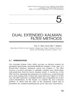
PSFisspace-vary ing. Thesupportofthespace-varyingPSFisindicatedbytheshadedareainFig.53.1,
wheretherectangle depictedbysolidlinesshowsthesupport of a low-resolutionpixeloverthe high-
resolutionsensorarray. The shaded region corresponds to the area swept bythelow-resolutionpixel
due to motion duringthe aperture time [8].
c

1999 by CRC Press LLC
FIGURE 53.1: Illustration of the discrete system PSF.
Note that the model (53.5) is invalid in case of occlusion. That is, each observed pixel (n
1
,n
2
; k)
canbe expressedas alinearcombinationofseveraldesiredhig h-resolutionpixels(m
1
,m
2
),provided
that (n
1
,n
2
; k) is connected to (m
1
,m
2

) by a motion trajectory. We assume that occlusion regions
can be detected a priori using a proper motion estimation/segmentation algorithm.
53.2.4 Regularization Models
Restorationisanill-posedproblemwhichcanberegularizedbymodelingcertainaspectsofthedesired
“ideal” image. Images can be modeled as either 2-D deterministic sequences or random fields. A
priori information about the ideal image can then be used to define hard or soft constraints on the
solution. In the deterministic case, images are usually assumed to be members of an appropriate
Hilbert space, such as aEuclidean space withthe usual inner productand norm. For example, in the
context of set theoretic restoration, the solution can be restricted to be a member of a set consisting
of all images satisfying a certain smoothness criterion [9]. On the other hand, constrained least
squares (CLS) and Tikhonov-Miller regularization use quadratic functionals to impose smoothness
constraints in an optimization framework.
In the random case, models have been developed for the pdf of the ideal image in the context of
maximuma posteriori(MAP)imagerestoration. Forexample, TrussellandHunt[10]haveproposed
a Gaussian distribution with space-varying mean and stationary covariance as a model for the pdf
of the image. Geman and Geman [11] proposed a Gibbsdistribution to model thepdf ofthe image.
Alternatively, if the image is assumed to be a realization of a homogeneous Gauss-Markov random
process,then it canbe statistically modeled through anautoregressive (AR) differenceequation [12]
f
(
n
1
,n
2
)
=

(
m
1

,m
2
)
∈
S
c
c
(
m
1
,m
2
)
f
(
n
1
− m
1
,n
2
− m
2
)
+ w
(
n
1
,n
2

)
(53.6)
where {c(m
1
,m
2
) : (m
1
,m
2
) ∈ S
c
} denote the model coefficients, S
c
is the model support (which
may be causal, semi-causal, or non-causal), and w(n
1
,n
2
) represents the modeling error which is
Gaussian distributed. The model coefficients can be determined such that the modeling error has
minimumvariance[12]. Extensionsof(53.6)toinhomogeneous Gauss-Markovfieldswasproposed
by Jeng and Woods [13].
53.3 Model Parameter Estimation
Inthissection,wediscussmethodsforestimatingtheparameters thatareinvolvedin theobservation
and regularization models for subsequent use in the restoration algorithms.
c

1999 by CRC Press LLC
53.3.1 Blur Identification

Blur identification refers to estimation of both the support and parameters of the PSF {d(n
1
,n
2
) :
(n
1
,n
2
) ∈ S
d
}. It is a crucialelement of image restoration because the quality of restored images is
highly sensitiveto errors in thePSF [14]. An early approach to blur identification has been based on
the assumption that the original scene contains an ideal point source, and that its spread (hence the
PSF) can be determined from the observed image. Rosenfeld and Kak [15] show that the PSF can
alsobedeterminedfromanidealline source. These approachesare oflimiteduse in practicebecause
a scene, in general, doesnot contain an ideal point or line source and the observation noise may not
allow the measurement of a useful spread.
Models for certain types of PSF can be derived using principles of optics, if the source of the
blur is known [7]. For example, out-of-focus and motion blur PSF can be parameterized with afew
parameters. Further,theyarecompletelycharacterizedbytheirzerosinthefrequency-domain. Power
spectrumandcepstrum(Fouriertransformofthelogarithmofthepowerspectrum)analysismethods
have been successfully applied in many cases to identify the location of these zero-crossings [ 16, 17].
Alternatively, Chang et al. [18] proposed a bispectrum analysis method, which is motivated by the
fact that bispectrum is not affected, in principle, by the observation noise. However, the bispectral
method requires much more data than the method based on the power spectrum. Note that PSFs,
whichdonothavezerocrossingsinthe frequencydomain(e.g., GaussianPSFmodeling atmospheric
turbulence), cannot be identified by these techniques.
Yetanotherapproachforbluridentificationisthemaximumlikelihood(ML)estimationapproach.
TheMLapproachaimstofind those parameter values (including, in pr inciple, theobservationnoise

variance) that have most likely resulted in the observed image(s). Different implementations of the
ML image and blur identification are discussed under a unifying framework [19]. Pavlovi
´
c and
Tekalp [20] proposea practical method to find theML estimates of thepar ameters of a PSFbased on
a continuous domain image formation model.
Inmulti-frameimagerestoration,bluridentificationusingmorethanoneframeatatimebecomes
possible. For example, the PSF of a possibly space-varying motion blur can be computed at each
pixel from an estimate of the frame-to-frame motion vector at that pixel, provided that the shutter
speed of the camera is known [21].
53.3.2 Estimation of Regularization Parameters
Regularizationmodelparameters aim to strikeabalancebetween the fidelityofthe restoredimage to
the observed data and its smoothness. Various methods exist to identify regularization parameters,
such as parametric pdf models, parametric smoothness constraints, and AR image models. Some
restoration methods require the knowledge of the power spectrum of the ideal image, which can be
estimated,forexample,fromanARmodeloftheimage. TheARparameterscan,inturn,beestimated
from the observed image by a least squares [22] or an ML technique [63]. On the other hand,
non-parametric spectral estimation is also possible through the application of periodogram-based
methodstoaprototypeimage[69,23]. Inthecontextofmaximumaposteriori(MAP)methods,thea
prioripdfisoftenmodeled by a parametricpdf,suchas a Gaussian [ 10] or a Gibbsian [11]. Standard
methods for estimating these parameters do not exist. Methods for estimating the regularization
parameter in the CLS, Tikhonov-Miller, and related formulations are discussed in [24].
53.3.3 Estimation of the Noise Variance
Almost all restoration algorithms assume that the observation noise is a zero-mean, white random
process that is uncorrelated with the image. Then, the noise field is completely characterized by its
variance, which is commonly estimated by the sample variance computed over a low-contrast local
c

1999 by CRC Press LLC
region of the observed image. As we will see in the following section, the noise variance plays an

important role in defining constraints used in some of the restoration algorithms.
53.4 Intra-Frame Restoration
Westartbyfirstlookingatsomebasicregularizedrestorationstrategies,inthecaseofanLSIblurmodel
withnopointwisenonlinearity. Theeffectofthenonlinearmappings(.)isdiscussedinSection53.4.2.
Methods that allow PSFs with a random components are summarized in Section 53.4.3. Adaptive
restoration for ringing suppression and blind restoration are covered in Sections 53.4.4 and 53.4.5,
respectively. Restoration of multispectral images and space-varyingblurred images are addressed in
Sections 53.4.6 and 53.4.7, respectively.
53.4.1 Basic Regularized Restoration Methods
When the mapping s(.) is ignored, it is evident from Eq. (53.1) that image restoration reduces to
solving a set of simultaneous linear equations. If the matrix D is nonsingular (i.e., D
−1
exists) and
the vector g lies in the column space of D (i.e., there is no observation noise), then there exists a
uniquesolutionwhichcanbefoundbydirect inversion(alsoknown as inversefiltering). In practice,
however,wealmostalwayshaveanunderdetermined(duetoboundarytruncationproblem[14])and
inconsistent(due to observation noise) setof equations. In this case,we resort to a minimum-norm
least-squaressolution. A least squares (LS) solution (notunique when the columns of D arelinearly
dependent) minimizes the norm-square of the residual
J
LS
(f )
.
=||g − Df ||
2
(53.7)
LS solution(s) with the minimum norm (energy) is (are) generally known as pseudo-inverse solu-
tion(s) (PIS).
Restorationbypseudo-inversionis oftenill-posed owingtothepresenceofobservationnoise[14].
This follows because the pseudo-inverse operator usually has some very large eigenvalues. For ex-

ample, a typical blur transfer function has zeros; and thus, its pseudo-inverse attains very large
magnitudes near these singularities as well as at high frequencies. This results in excessive amplifi-
cation at these frequencies in the sensor noise. Regularized inversion techniques attempt to roll-off
the transfer function of the pseudo-inverse filter at these frequencies to limit noise amplification.
It follows that the regularized inverse deviates from the pseudo-inverse at these frequencies which
leads to other types of artifacts, generally known as regularization artifacts [14]. Various strategies
for regularized inversion (and how to achieve the right amount of regularization) are discussed in
the following.
Singular-Value Decomposition Method
The pseudo-inverse D
+
can be computed using the singular value decomposition (SVD) [1]
D
+
=
R

i=0
λ
−1/2
i
z
i
u
T
i
(53.8)
where λ
i
denote the singular values, z

i
and u
i
are the eigenvectors of D
T
D and DD
T
, respectively,
andR isthe rankofD. Clearly,reciprocation ofzerosingular-valuesisavoidedsince thesummation
runs to R, the rank of D. Under the assumption that D is block-circulant (corresponding to a
circular convolution), the PIS computed through Eq. (53.8) is equivalent to the frequency domain
c

1999 by CRC Press LLC
pseudo-inverse filtering
D
+
(u, v) =

1/D(u, v) if D(u, v) = 0
0 if D(u, v) = 0
(53.9)
where D(u, v) denotes the frequency response of the blur. This is because a block-circulant matrix
can be diagonalized by a 2-D discrete Fourier transformation (DFT) [2].
Regularization of the PIS can then be achieved by truncating the singular value expansion (53.8)
to eliminate all terms corresponding to small λ
i
(which are responsible for the noise amplification)
at the expense of reduced resolution. Truncation str ategies are generally ad-hoc in the absence of
additional information.

Iterative Methods (Landweber Iterations)
Several image restoration algorithmsare based on variations of the so-called Landweber itera-
tions [25, 26, 27, 28, 31, 32]
f
k+1
= f
k
+ RD
T

g − Df
k

(53.10)
where R is a matrix that controls the rate of convergence of the iterations. There is no general way
to select the best C matrix. If the system (53.1) is nonsingular and consistent (hardly ever the case),
the iterations (53.10) willconverge to the solution. If, on the otherhand, (53.1) is underdetermined
and/or inconsistent, then (53.10) converges to a minimum-norm least squares solution (PIS). The
theory of this and other closely related algorithms are discussed by Sanz and Huang [26] and Tom
et al. [27]. Kawata and Ichioka [28] are among the first to apply the Landweber-type iterations to
image restoration, which they refer to as “reblurring” method.
Landweber-type iterative restoration methods can be regularized by appropriately terminating
the iterations before convergence, since the closer we are to the pseudo-inverse, the more noise
amplification we have. A termination rule can be defined on the basis of the norm of the residual
image signal [29]. Alternatively, soft and/or hard constraints can be incorporated into iterations to
achieve regularization. Theconstrained iterations can be written as [30, 31]
f
k+1
= C


f
k
+ RD
T

g − Df
k


(53.11)
whereC is a nonexpansiveconstraint operator, i.e., ||C(f
1
) − C(f
2
)||≤||f
1
− f
2
||, to guarantee
theconvergenceoftheiterations. ApplicationofEq.(53.11)toimagerestorationhasbeenextensively
studied (see [31, 32] and the references therein).
Constrained Least Squares Method
Regularizedimagerestorationcanbeformulatedasaconstrainedoptimizationproblem,where
a functional ||Q(f )||
2
of the image is minimized subject to the constraint ||g − Df ||
2
= σ
2
.Here

σ
2
is a constant, which isusually setequal to the variance of the observation noise. The constrained
least squares (CLS) estimate minimizes the Lagrangian [34]
J
CLS
(f ) =||Q(f )||
2
+ α

||g − Df ||
2
− σ
2

(53.12)
whereα istheLagrangemultiplier. TheoperatorQ ischosensuchthattheminimizationofEq.(53.12)
enforces some desired property of the ideal image. For instance, if Q is selected as the Laplacian
operator, smoothnessoftherestoredimageisenforced. TheCLSestimatecanbeexpressed,bytaking
the derivative of Eq. (53.12) and setting it equal to zero, as [1]
ˆ
f =

D
H
D + γ Q
H
Q

−1

D
H
g (53.13)
c

1999 by CRC Press LLC
where
H
stands for Hermitian (i.e., complex-conjugate and transpose). The parameter γ =
1
α
(the
regularization parameter) must be such that the constraint ||g − Df ||
2
= σ
2
is satisfied. It is often
computed iteratively [2]. A sufficient condition for the uniqueness of the CLS solution is that Q
−1
exists. For space-invariant blurs, the CLS solution canbe expressed in the frequency domain as [34]
ˆ
F (u, v) =
D
∗
(u, v)
|D(u, v)|
2
+ γ |L(u, v)|
2
G(u, v) (53.14)

where
∗
denotescomplexconjugation. AcloselyrelatedregularizationmethodistheTikhonov-Miller
(T-M)regularization[33,35]. T-Mregularization has beenappliedtoimagerestoration[31, 32,36].
Recently, neural network structures implementingthe CLS or T-M image restoration have also been
proposed [37, 38].
Linear Minimum Mean Square Error Method
The linear minimum mean square error (LMMSE) method finds the linear estimate which
minimizes the mean square error between the estimate and ideal image, using up to second order
statistics of the ideal image. Assumingthat the ideal imagecan bemodeled bya zero-meanhomoge-
neous random fieldand the bluris space-invariant, theLMMSE (Wiener) estimate, in thefrequency
domain, is given by [8]
ˆ
F (u, v) =
D
∗
(u, v)
|D(u, v)|
2
+ σ
2
v
/|P (u, v)|
2
G(u, v) (53.15)
where σ
2
v
is the variance of the observation noise (assumed white) and |P (u, v)|
2

stands for the
powerspectrum of the ideal image. The powerspectrumofthe ideal image is usually estimated from
a prototype. It can be easily seen that the CLS estimate (53.14) reduces to the Wiener estimate by
setting |L(u, v)|
2
= σ
2
v
/|P (u, v)|
2
and γ = 1.
A Kalman filter determines the causal (up to a fixed lag) LMMSE estimate recursively. It is based
on a state-space representation of the image and observ ation models. In the first step of Kalman
filtering, a prediction of the present state is formed using an autoregressive (AR) image model and
the previous state of the system. In the second step, the predictions are updated on the basis of the
observed image data to form the estimate of the present state. Woods and Ingle [39] applied 2-D
reduced-updateKalmanfilter (RUKF)toimagerestoration, wherethe updateislimited toonly those
state variables in a neighborhood of the present pixel. The main assumption here is that a pixel is
insignificantly correlated with pixels outside a certain neighborhood about itself. More recently, a
reduced-ordermodelKalmanfiltering(ROMKF),wherethestatevectoristruncatedtoasizethatison
the order of the image modelsupport has beenproposed [40]. Other Kalmanfiltering formulations,
including higher-dimensional state-space models to reduce the effective size of the state vector, have
been reviewed in [7]. The complexity of higher-dimensional state-space model based formulations,
however, limits their pr actical use.
Maximum A posteriori Probability Method
Themaximumaposterioriprobability(MAP)restorationmaximizestheaposterioriprobability
density function (pdf) p(f |g), i.e., the likelihood of a realization of f being the ideal image given
the observed data g. Through the application of the Bayes rule, we have
p(f |g) ∝ p(g|f )p(f )
(53.16)

wherep(g|f ) istheconditionalpdf of g givenf (relatedtothe pdf of the noise process)and p( f )is
the a priori pdf oftheideal image. Weusuallyassume that the observation noise is Gaussian,leading
c

1999 by CRC Press LLC
to
p(g|f ) =
1
(
2π
)
N/2
|R
v
|
1/2
exp

−1/2
(
g − Df
)
T
R
−1
v
(
g − Df
)


(53.17)
whereR
v
denotes the covariancematrix of the noise process. Unlike the LMMSEmethod, theMAP
method uses complete pdf information. However, if both the image and noise are assumed to be
homogeneous Gaussian random fields, the MAP estimate reduces to the LMMSE estimate, under a
linear observation model.
Trusselland Hunt [10] used non-stationarya prioripdf models, andproposeda modifiedform of
thePicarditerationtosolvethe nonlinear maximizationproblem. They suggestedusingthe variance
of the residualsignal as a criterionforconvergence. Geman and Geman[11] proposedusing a Gibbs
randomfield modelforthea prioripdfoftheidealimage. Theyusedsimulatedannealingprocedures
to maximize Eq. (53.16). It should be noted that the MAP procedures usually require significantly
more computation compared to, for example, the CLS or Wiener solutions.
Maximum Entropy Method
A number of maximum entropy(ME) approacheshavebeen discussed in theliterature,which
vary in the way that the ME principle is implemented. A common feature of all these approaches,
however, is their computational complexity. Maximizing the entropy enforces smoothness of the
restored image. (In the absence of constraints, the entropy is highest for a constant-valued image).
One importantaspect of the ME approach is that the nonnegativity constraint isimplicitly imposed
on the solution because the entropy is defined in terms of the logarithm of the intensity.
Frieden was the first to apply the ME principle to image restoration [41]. In his formulation, the
sum of the entropy of the image and noise, given by
J
ME1
(f ) =−

i
f(i)ln f(i)−

i

n(i) ln n(i) (53.18)
is maximized subject to the constraints
n = g − Df
(53.19)

i
f(i) = K
.
=

i
g(i) (53.20)
which enforce fidelity to the dataand a constantsum of pixel intensities. This approach requires the
solution of a system of nonlinear equations. The number of equations and unknowns are on the
order of the number of pixels in the image. The formulation proposed by Gull and Daniell [42] can
be viewed as another form of Tikhonov regularization (or constrained least squares formulation),
where the entropy of the image
J
ME2
(f ) =−

i
f(i)ln f(i) (53.21)
is the regularization functional. It is maximized subject to the following usual constraints
||g − Df ||
2
= σ
2
v
(53.22)


i
f(i)= K
.
=

i
g(i) (53.23)
on the restored image. The optimization problem is solved using an ascent algorithm. Trussell [43]
showed that in the case of a prior distribution defined in terms of the image entropy, the MAP
solution is identical to the solution obtained by this ME formulation. Other ME formulations were
also proposed [44, 45]. Note that all ME methods are nonlinear in nature.
c

1999 by CRC Press LLC
Set-Theoretic Methods
Inset-theoreticmethods,firstanumberof“constraintsets”aredefinedsuchthattheirmembers
are consistent withthe observations and/or some a priori information about the ideal image. A set-
theoretic estimate of the ideal image is then defined as a feasible solution satisfying all constraints,
i.e., any member of the intersection of the constraint sets. Note that set-theoretic methods are, in
general, nonlinear.
Set-theoretic methods vary according to the mathematical properties of the constraint sets. In
the method of projections onto convex sets (POCS),the constraint sets C
i
are closed and convex in
an appropriate Hilbert space H. Given the sets C
i
, i = 1, ,M, and their respective projection
operators P
i

, a feasible solution is found by performing successive projections as
f
k+1
= P
M
P
M−1
P
1
f
k
; k = 0, 1, (53.24)
wheref
0
istheinitialestimate(apointinH). Theprojectionoperators areusuallyfoundbysolving
constrained optimization problems. In finite-dimensional problems (which is the case for dig ital
image restoration), the iterations converge to a feasible solution in the intersection set [46, 47, 48].
Itshould be noted that theconvergencepoint is affected by the choiceof the initialization. However,
as the size of the intersection set becomes smaller, the differences between the convergence points
obtained by different initializations become smaller. Trussell and Civanlar [49] applied POCS to
imagerestoration. Forexamplesofconvexconstraintsetsthatareusedinimage restoration,see[23].
A relationship between the POCS and Landweber iterations were developed in [10].
A special case of POCS is the Gerchberg-Papoulis type algorithms where the constraint sets are
either linear subspaces or linear varieties [50]. Extensions of POCS to the case of nonintersecting
sets [51] and nonconvex sets [52] have been discussed in the literature. Another extension is the
method of fuzzy sets (FS), where the constraints are defined in terms of FS. More precisely, the
constraintsarereflectedinthemembershipfunctionsdefiningtheFS.Inthiscase,afeasiblesolutionis
definedasonethathasahighgradeofmembership(e.g.,aboveacertainthreshold)intheintersection
set. The method of FS has also been applied to image restoration [53].
53.4.2 Restoration of Images Recorded by Nonlinear Sensors

Image sensors and media may have nonlinear characteristics that can be modeled by a pointwise
(memoryless) nonlinearity s(.). Common examples are photographic film and paper, where the
nonlinear relationship between the exposure (intensity)and the silver densitydeposited on the film
orpaperis specifiedbya“d − loge”curve. The modelingofsensornonlinearitieswasfirstaddressed
by Andrews and Hunt [1]. However, it was not generally recognized that results obtained by taking
the sensor nonlinearity into account may be far more superior to those obtained by ignoring the
sensor nonlinearity, until the experimental work of Tekalp and Pavlovi
´
c[54, 55].
ExceptfortheMAPapproach,noneofthealgorithmsdiscussedaboveareequippedtohandlesensor
nonlinearity in a straightforward fashion. A simple approach would be to expand the observation
modelwiths(.) intoitsTaylorseriesaboutthemeanoftheobservedimageandobtainanapproximate
(linearized)model,whichcanbeusedwithanyoftheabovemethods[1]. However, theresultsdonot
show significant improvement over those obtained by ignoring the nonlinearity. The MAP method
is capable of taking the sensor nonlinearity into account directly. A modified Picard iteration was
proposedin[10], assuming both the image and noise are Gaussian distributed, which is given by
ˆ
f
k+1
=
¯
f
k
+ R
f
D
T
S
b
R

−1
n

g − s

Df
k

(53.25)
where
¯
f denotes non-stationary image mean, R
f
and R
n
are the correlation matrices of the ideal
imageandnoise,respectively,andS
b
isadiagonalmatrixconsistingofthederivativesofs(.) evaluated
c

1999 by CRC Press LLC
atb = Df . ItisthematrixS
b
thatmapsthedifference[g − s(Df
k
)] fromthe observationdomain
to the intensity domain.
An alternative approach, which is computationally less demanding, transforms the observed den-
sity domain image to the exposure domain [54]. There is a convolutional relationship between

the ideal and blurred images in the exposure domain. However, the additive noise in the density
domain manifests itself as multiplicative noise in the exposure domain. To this effect, Tekalp and
Pavlovi
´
c[54] derive an LMMSE deconvolution filter in the presence of multiplicative noise under
certainassumptions. Theirresultsshowthataccountingforthesensornonlinearitymaydramatically
improve restoration results [54, 55].
53.4.3 Restoration of Images Degraded by Random Blurs
Basic regularized restoration methods (reviewed in Section 53.4.1) assume that the blur PSF is a
deterministic function. A more realistic model may be
D =
¯
D + D
(53.26)
where
¯
D is the deterministic part(known or estimated) of the blur operator andD stands for the
random component. Random component may represent inherent random fluctuations in the PSF,
for instance due to atmospheric turbulence or random relative motion, or it may model the PSF
estimation error.
A naive approach would be to employ the expected value of the blur operator in one of the
restoration algorithms discussed above. The resulting restoration, however, may be unsatisfactor y.
Slepian [56] derived the LMMSE estimate, which explicitly incorporated the randomcomponent of
the PSF. The resulting Wiener filter requires the a priori knowledge of the second order statistics of
theblurprocess. Wardetal. [57, 58] also proposedLMMSEestimators. Combettesand Trussell[59]
addressedrestorationofrandomblurswithintheframeworkofPOCS,wherefluctuations inthePSF
are reflected in the bounds defining the residual constraint sets. The method of total least squares
(TLS) has beenusedin the mathematicsliteraturetosolvea set oflinearequations withuncertainties
in the system matr ix. The TLSmethod amounts to findingthe minimum perturbations on D and g
to make the system of equations consistent. A variation of this principle has been applied to image

restoration with random PSF by Mesarovic et al. [60]. Various authors have shown that modeling
the uncertaintyin the PSF(bymeans of a random component)reducesringing artifacts that are due
to using erroneous PSF estimates.
53.4.4 Adaptive Restoration for Ringing Reduction
Linear space-invariant (LSI) restoration methods introduce disturbing ringing artifacts which orig-
inate around sharp edgesand image borders [36]. A quantitative analysis of the origins and charac-
teristics of ringing and other restoration artifacts was given by Tekalp and Sezan [14]. Suppression
of ringing may be possible by means of adaptivefiltering, which tracks edges or imagestatistics such
as local mean and variance.
Iterative and set-theoretic methods are well-suited for adaptive image restoration with r inging
reduction. Lagendijketal.[ 36]haveextendedMillerregularizationtoadaptiverestorationbydefining
thesolutioninaweightedHilbertspace,intermsofnormsweightedbyspace-variant weights. Later,
SezanandTekalp[9]extendedthemethodofPOCStothespace-variantcasebyintroducingaregion-
based bound on the signal energy. In both methods, the weights and/or the regions were identified
from the degraded image. Recently, Sezan and Trussell [23] have developed constraints based on
prototype images for set-theoretic image restoration withartifact reduction.
Kalman filtering can also be extended to adaptive image restoration. For a typical image, the
homogeneity assumption will hold only over small regions. Rajala and de Figueiredo [61] used an
c

1999 by CRC Press LLC
off-line visibilit y function to segment the image according to the local spatial activity of the picture
being restored. Later, a rapid edge adaptive filter based on multiple image models to account for
edges withvariousorientations was developed by Tekalpet al. [62]. Jengand Woods [13] developed
inhomogeneous Gauss-Markov field models for adaptive filtering, and maximum entropy methods
were used for ringing reduction [45]. Results show a significant reduction in ringing artifacts in
comparison to LSI restoration.
53.4.5 Blind Restoration (Deconvolution)
Blind restoration refers to methods that do not require prior identification of the blur and regular-
ization model parameters. Two examples are simultaneous identification and restoration of noisy

blurred images [63] and image recovery from Fourier phase information [64]. Lagendijk et al. [63]
appliedtheE-M algorithmtoblindimage restoration,whichalternatesbetweenMLparameteriden-
tification and minimum mean square error image restoration. Chen et al. [64] employed the POCS
method to estimatethe Fourier magnitude of the ideal image fromtheFourierphase of the observed
blurred image by assuming a zero-phase blur PSF so that the Fourier phase of the observed image is
undistorted. Both methods require the PSF to be real and symmetric.
53.4.6 Restoration of Multispectral Images
Atrivial solutionto multispectral image restoration, when there is no inter-bandblurring, may be to
ignore the spectral correlations among different bands and restore each band independently, using
oneofthealgor ithmsdiscussedabove. However,algorithmsthatareoptimalforsingle-bandimagery
may no longer be so when applied to individual spectral bands. For example, restoration of the red,
green, and blue bands of a color image independently usually results in objectionable color shift
artifacts.
To this effect, Hunt and Kubler [65] proposed employing the Karhunen-Loeve (KL) transfor m
to decorrelate the spectral bands so that an independent-band processing approach can be applied.
However, because the KL transform is image dependent, they then recommended using the NTSC
YIQ transformation as a suboptimum but easy-to-use alternative. Experimental evidence shows
that the visual quality of restorations obtained in the KL, YIQ, or another luminance-chrominance
domain are quite similar [65]. In fact, restoration of only the luminance channel suffices in most
cases. Thismethodappliesonlywhenthereisnointer-bandblurring. Further,oneshouldrealizethat
the observation noise becomes correlated with the image under a non-orthogonal transformation.
Thus,filteringbasedon the assumptionthattheimage and noiseareuncorrelatedisnot theoretically
founded in the YIQ domain.
Recent efforts in multispectral image restoration are concentrated on making total use of the
inherent correlations between the bands [66, 67]. Applying the CLS filter expression (53.13)tothe
observation model (53.4) with Q
H
Q = R
−1
f

R
v
, we obtain the multispectral Wiener estimate
ˆ
f ,
givenby[68]
ˆ
f =

D
T
D + R
−1
f
R
v

−1
D
T
g (53.27)
where
R
f
.
=






R
f ;11
··· R
f ;1K
.
.
.
.
.
.
.
.
.
R
f ;K1
··· R
f ;KK





, and R
v
.
=






R
v;11
··· R
v;1K
.
.
.
.
.
.
.
.
.
R
v;K1
··· R
v;KK





Here R
f ;ij
.
= E{f
i
f

T
j
} and R
v;ij
.
= E{v
i
v
T
j
}, i, j = 1, 2, ,K denote the inter-band, cross-
correlation matrices. Note that if R
f ;ij
= 0 for i = j, i, j = 1, 2, ,K, then the multiframe
c

1999 by CRC Press LLC
estimate becomes equivalent to stacking the K single-frame estimates obtained independently.
Directcomputationof
ˆ
f through Eq. (53.27) requiresinversionof a N
2
L × N
2
L matrix. Because
the blur PSF is not necessarily the same in each band and the inter-band correlations are not shift-
invariant,thematricesD, R
f
,andR
v

arenotblock-Toeplitz;thus,a3-DDFTwouldnotdiagonalize
them. However, assuming LSI blurs, each D
k
is block Toeplitz. Furthermore, assuming each image
and noise band are wide-sense stationary, R
f ;ij
and R
v;ij
are also block-Toeplitz. Approximating
the block-Toeplitz submatrices D
i
, R
f ;ij
, andR
v;ij
by block-circulant ones, each submatrix can be
diagonalized by a separate 2-D DFT operation so that we only need to invert a block matrix with
diagonal sub-blocks. Galatsanos and Chin [66] proposed a method that successively partitions the
matrix tobeinvertedand recursivelycomputestheinverseofthesepartitions. LaterOzkan et al.[68]
has shown that the desired inverse can be computed by inverting N
2
submatrices, each K × K,in
parallel. The resulting numerically stable filter was called the cross-correlated multiframe (CCMF)
Wiener filter.
The multispectral Wiener filter requires the knowledge of the correlation matrices R
f
and R
v
.
If we assume that the noise is white and spectrally uncorrelated, the matrix R

v
is diagonal with all
diagonalentriesequaltoσ
2
v
. EstimationofthemultispectralcorrelationmatrixR
f
canbeperformed
by either the periodogram method or 3-D AR modeling [68]. Sezan and Trussell [69] show that the
multispectral Wiener filter is highly sensitive to the cross-power spectral estimates, which contain
phase information. Other multispectral restoration methods include Kalman filtering approach of
TekalpandPavlovi
´
c[67],leastsquaresapproachesofOhyamaetal.[70]andGalatsanosetal.[71],and
set-theoreticapproachof SezanandTrussell[23, 69] whoproposedmultispectral image constraints.
53.4.7 Restoration of Space-Varying Blur red Images
Inprinciple,allbasicregularizationmethodsapplytotherestorationofspace-varyingblurredimages.
However, because Fourier transforms cannot be utilized to simplify large matrix operations (such
as inversion or singular value decomposition) when the blur is space-varying, implementation of
some ofthese algorithms may be computationally formidable. There exist three distinct approaches
to attack the space-variant restoration problem: (1) sectioning, (2) coordinate transformation, and
(3) direct approaches.
The main assumption in sectioning is that the blur is approximately space-invariant over small
regions. Therefore, a space-varying blurred image can be restored by applying the well-known
space-invariant techniques to local image regions. Trussell and Hunt [73] propose using iterative
MAP restoration within rectangular, overlapping regions. Later, Trussell and Fo gel proposed using
a modified Landweber iteration [21]. A major drawback of sectioning methods is generation of
artifacts at the region boundaries. Overlapping the contiguous regions somewhat reduces these
artifacts, but does not completely suppress them.
Most space-varying PSF vary continuously from pixel to pixel (e.g., relative motion with acceler-

ation) violating the basic premise of the sectioning methods. To this effect, Robbins et al. [74] and
then Sawc huck [75] proposed a coordinate transformation (CTR) method such that the blur PSF in
the transformed coordinates is space-invariant. Then, the transformed image can be restored by a
space-invariant filter and then transformed back to obtain the final restored image. However, the
statisticalpropertiesoftheimageandnoiseprocessesareaffected bytheCTR,whichshouldbetaken
intoaccountin restorationfilterdesign. The results reported in [74] and [75] have been obtained by
inverse filtering; and thus, this statistical issue was of no concern. Also note that the CTR method is
applicable to a limited class of space-varying blurs. Forinstance,blurring duetodepth of field isnot
amenable to CTR.
The lack of generality of sectioning and CTR methods motivates direct approaches. Iterative
schemes, Kalman filtering, and set-theoretic methods can be applied to restoration of space-varying
c

1999 by CRC Press LLC
blurs in a computationally feasible manner. Angel and Jain [76] propose solving the superposition
Eq.(53.3)iterativelyusingaconjugategradientmethod. Applicationofconstrainediterativemethods
wasdiscussedin[30]. Morerecently,Ozkanetal.[72]developedarobustPOCSalgorithmforspace-
varying image restoration, where they defined a closed, convex constraint set for each observed
blurred image pixel (n
1
,n
2
),givenby:
C
n
1
,n
2
=


y :|r
(y)
(n
1
,n
2
)|≤δ
0

(53.28)
and
r
(y)
(
n
1
,n
2
)
.
= g
(
n
1
,n
2
)
−

(

m
1
,m
2
)
∈
S
d
(
n
1
,n
2
)
d
(
n
1
,n
2
; m
1
,m
2
)
y
(
m
1
,m

2
)
(53.29)
is the residual at pixel (n
1
,n
2
) associated with y, which denotes an arbitrary member of the set.
The quantityδ
0
is ana priori bound reflecting the statistical confidence with which the actual image
is a member of the set C
n
1
,n
2
. Since r
(f )
(n
1
,n
2
) = v(n
1
,n
2
), the bound δ
0
is determined from
the statistics of the noise process so that the ideal image is a member of the set within a certain

statisticalconfidence. The collectionofboundedresidualconstraints overall pixels(n
1
,n
2
) enforces
the estimate to be consistent with the observed image.
Theprojectionofanarbitraryx(i
1
,i
2
) onto each C
n
1
,n
2
is defined as:
P
n
1
,n
2
[
x
(
i
1
,i
2
)
]

=











x
(
i
1
,i
2
)
+
r
(x)
(
n
1
,n
2
)
−δ
0


o
1

o
2
h
2
(
n
1
,n
2
;o
1
,o
2
)
h
(
n
1
,n
2
; i
1
,i
2
)
if r

(x)
(
n
1
,n
2
)
>δ
0
x
(
i
1
,i
2
)
if − δ
0
≤ r
(x)
(
n
1
,n
2
)
≤ δ
0
x
(

i
1
,i
2
)
+
r
(x)
(
n
1
,n
2
)
+ δ
0

o
1

o
2
h
2
(
n
1
,n
2
; o

1
,o
2
)
h
(
n
1
,n
2
; i
1
,i
2
)
if r
(x)
(
n
1
,n
2
)
< −δ
0
(53.30)
The algorithm starts with an arbitrary x(i
1
,i
2

), and successively projects onto each C
n
1
,n
2
. This is
repeated until convergence [72]. Additional constraints, such as bounded energy, amplitude, and
limited support, can be utilized to improve the results.
53.5 Multiframe Restoration and Superresolution
Multiframerestorationreferstoestimatingtheidealimageonalatticethatisidenticalwiththeobser-
vation lattice, whereas superresolution refers to estimating it on a lattice that has a higher sampling
density than the observation lattice. They both employ the multiframe observation model (53.5),
which establishes a relation between the ideal image and obser v ations at more than one instance.
Several authors eluded that the sequential nature of video sources can be statistically modeled by
means of temporal correlations [68, 71]. Multichannel filters similar to those described for multi-
spectral restoration were thus proposed for multiframe restoration. Here, we only review motion-
compensated (MC) restoration and superresolution methods, because they are more effective.
53.5.1 Multiframe Restoration
The sequential nature of imagesin a video source can beused to better estimate the PSFparameters,
regularization terms, and the restored image. For example, the extent of a motion blur can be
estimated from interframe motion vectors, provided that the aperture time is known. The first MC
approach was the motion-compensated multiframe Wiener filter (MCMF) proposed by Ozkan et
al.[68]whoconsideredthecaseofframe-to-frameglobal translations. Then, the autopowerspectra
c

1999 by CRC Press LLC
of all frames are the same and the cross spectra are related by a phase factor which can be estimated
from the motion information. Given the motion vectors (one for each frame) and the auto power
spectrum of the reference frame, theyderived a closed-form solution, given by
ˆ

F
k
(u, v) =
S
f ;k
(u, v)
N

i=1
S
∗
f ;i
(u, v)D
∗
i
(u, v)G
i
(u, v)
N

i=1
|S
f ;i
(u, v)D
i
(u, v)|
2
+ σ
2
v

, (53.31)
where k is the index of the ideal frame to be restored, N is the number of available frames, and
P
f ;ki
(u, v) = S
f ;k
(u, v)S
∗
f ;i
(u, v) denotes the cross power spectrum between the frames k and i
in factored form. The fact that such a factorization exists was shown in [68] for the case of global
translational motion. The MCMF yields the biggest improvement when the blur PSF changes from
frame-to-frame. Thisisbecausethesummationinthedenominatormaynotbezeroatanyfrequency,
eventhougheachtermD
i
(u, v) mayhavezerosatcertainfrequencies. Thecaseofspace-varyingblurs
maybeconsideredasaspecialcaseofthelastsectionwhichcoverssuperresolutionwithspace-varying
restoration.
53.5.2 Superresolution
When the interframe motion is subpixel, each frame, in fact, contains some “new” information that
can be utilized to achieve superresolution. Superresolution refers to high-resolution image expan-
sion,whichaimstoremovealiasingartifacts,blurringduetosensorPSF,andopticalblurringgiventhe
observation model (53.5). Provided that enough frames with subpixel motion are available, the ob-
servationmodelbecomesinvertible. Itcanbeeasilyseen,however,thatsuper resolutionfromasingle
observedimageisill-posedbecausewehavemoreunknownsthanequations,andthereexistinfinitely
manyexpandedimages that are consistent with themodel (53.5). Therefore, single-frame nonlinear
interpolation (also called image expansion and digital zooming) methods for improved definition
imageexpansionemployadditionalregularizationcr iteria, suchasedge-preservingsmoothness con-
straints [77,78]. (Itis well-known thatno new high-frequency information canbe generated by LSI
interpolation techniques, including ideal band-limited interpolation, hence the need for nonlinear

methods.)
Severalearlymotion-compensatedmethodsarein theformoftwo-stageinterpolation-restoration
algorithms[79,80]. Theyarebasedonthepremisethatpixelsfromallobservedframescanbemapped
backontoa desiredframe, based on estimatedmotiontrajectories, toobtainanupsampledreference
frame. However, unless we assume global translational motion, the upsampled reference frame is
nonuniformly sampled. Inordertoobtaina uniformly spaced upsampled image,interpolationonto
a uniform sampling grid needs to be performed. Image restoration is subsequently applied to the
upsampled image to remove the effect of the sensor blur. However, these methods do not use an
accurate image formation model, and cannot remove aliasing ar tifacts.
Motion-compensated (multiframe) superresolution methods that are based on the model (53.5)
canbeclassifiedasthosethataimtoeliminate(1)aliasingonly,(2)aliasingandLSIblurs,and(3)alias-
ingand space-varyingblurs. Inaddition, someofthese methodsaredesignedforglobaltr anslational
motiononly,while otherscanhandle space-varyingmotion fieldswithocclusion. Multiframesuper-
resolution was first introduced by Tsai and Huang [81] who exploited the relationship between the
continuous and discrete Fourier transforms of the undersampled frames to remove aliasing errors,
in the special case ofglobal motion. Their formulation has been extendedby Kim et. al. [82]to take
into account noise and blur in the low-resolution images, byposing theproblem in the least squares
sense. A further refinement by Kim and Su [83] allowed blurs that are different for each frame of
c

1999 by CRC Press LLC
low-resolution data, by using a Tikhonov regularization. However, the resulting algorithm did not
treat the formationof blur due to motion or sensor size, and suffers from convergence problems.
Inspection of the model (53.5) suggests that the superresolution problem can be stated in the
spatio-temporal domain as the solution of a set of simultaneous linear equations. Suppose that
the desired high-resolution frames are M × M, and we have L low-resolution observations, each
N × N . Then, from Eq. (53.5), we can set up at most L × N × N equations in M
2
unknowns to
reconstruct a particular hig h-resolution frame. These equations are linearly independent provided

that all displacements between the successive frames are at subpixel amounts. (Clearly, the number
of equations will be reduced by the number of occlusion labels encountered along the respective
motion trajectories.) In general, it is desirableto set up an overdetermined system of equations, i.e.,
L>R
2
= M
2
/N
2
,toobtainamorerobustsolutioninthepresenceofobservationnoise. Becausethe
impulse response coefficients h
ik
(n
1
,n
2
; m
1
,m
2
) are spatially varying, and hence the system matrix
is not block-Toeplitz, fast methods to solve them are not available. Stark and Oskui [86] proposed
a POCS method to compute a high resolution image from observations obtained by translating
and/or rotating an image w ith respect to a CCD array. Irani and Peleg [84, 85] employed iterative
methods. Pattiet al. [87] extended the POCSformulation to include sensornoise and space-varying
blurs. Bayesianapproacheswerealsoemployedforsuperresolution [88]. Theextensionof thePOCS
method with space-varying blurs is explained in the following.
53.5.3 Superresolution with Space-Varying Restoration
The POCS method described here addresses the most general form of the superresolution problem
based on the model (53.5). The formulation is quite similar to the POCS approach presented for

intraframe restoration of space-varying blurred images. In this case, we define a different closed,
convex set for each observed low-resolutionpixel (n
1
,n
2
,k)(which can be connected to the desired
frame i by a motion trajectory)as
C
n
1
,n
2
;i,k
=

x
i
(
m
1
,m
2
)
:|r
(x
i
)
k
(
n

1
,n
2
)
|≤δ
0

, 0 ≤ n
1
,n
2
≤ N − 1,k= 1, ,L (53.32)
where
r
(
x
i
)
k
(n
1
,n
2
)
.
= g
k
(
n
1

,n
2
)
−
M−1

m
1
=0
M−1

m
2
=0
x
i
(
m
1
,m
2
)
h
ik
(
m
1
,m
2
; n

1
,n
2
)
and δ
0
represents the confidence that we have in the observation and is set equal to cσ
v
,whereσ
v
is
the standard deviation of the noise and c ≥ 0 is determined by an appropriate statistical confidence
bound. Thesesetsdefinehigh-resolutionimagesthatareconsistentwiththeobservedlow-resolution
frames within a confidence bound that is proportional to the variance of the observation noise. The
projection operator which projects onto C
n
1
,n
2
;i,k
can be deduced from Eq. (53.30)[8]. Additional
constraints,suchasamplitudeand/orfinitesupportconstraints,canbeutilizedtoimprovetheresults.
Excellent reconstructions have been reported using this procedure [ 68, 87].
A few observations about the POCS method are in order: (1) While certain similarities exist
between the POCS iterations and the Landweber-typeiterations [79, 84, 85], the POCSmethod can
adapttotheamountoftheobservationnoise,whilethelattergenerallycannot. (2)ThePOCSmethod
finds a feasible solution, that is, a solution consistent with all available low-resolution observations.
Clearly, the moreobservations(moreframeswithreliablemotion estimation)wehave,thebetterthe
high-resolution reconstructed image ˆs
i

(m
1
,m
2
) willbe. Ingeneral, itis desirable thatL>M
2
/N
2
.
Note,however,thatthePOCSmethodgeneratesareconstructedimagewithanynumberL ofavailable
frames. Thenumber L isjust anindicatorofhowlargethefeasibleset ofsolutionswillbe. Ofcourse,
the size of the feasible set can be further reduced by employing other closed, convex constraints in
the form of statistical or structural image models.
c

1999 by CRC Press LLC
53.6 Conclusion
Atpresent,factorsthatlimitthesuccessofdigitalimagerestorationtechnologyincludelackofreliable
(1) methods for blur identification, especially identification of space-variant blurs, (2) methods to
identify imaging system nonlinearities, and (3) methods to deal with the presence of artifacts in
restored images. Our experience with the restoration of real-life blurred images indicates that the
choice of a par ticular regularization strategy (filter) has a small effect on the qualit y of the restored
images as long as the parameters of the degradation model, i.e., the blur PSF and the SNR, and any
imagingsystemnonlinearityisproperlycompensated. Propercompensationofsystemnonlinearities
also plays a sig nificant role in blur identification.
References
[1] Andrews, H.C. and Hunt, B.R., Digital Image Restoration, Prentice-Hall, Englewood Cliffs,
NJ, 1977.
[2] Gonzales, R.C. and Woods, R.E.,
Digital Image Processing, Addison-Wesley, MA, 1992.

[3] Katsaggelos, A.K., Ed.,
Digital Image Restoration, Springer-Verlag,Berlin, 1991.
[4] Meinel,E.S., Origins oflinear andnonlinear recursiverestorationalgorithms,
J. Opt. Soc. Am.,
A-3(6), 787–799, 1986.
[5] Demoment, G.,Imagereconstructionandrestoration: Overviewofcommonestimationstruc-
tures and problems,
IEEE Trans. Acoust. Speech Sign. Proc., 37, 2024-2036, 1989.
[6] Sezan, M.I. and Tekalp, A.M., Survey of recent developments in digital image restoration,
Optical Eng., 29, 393–404, 1990.
[7] Kaufman, H. and Tekalp, A.M., Survey of estimation techniques in image restoration,
IEEE
Control Systems Magazine,
11, 16–24, 1991.
[8] Tekalp, A.M.,
Digital Video Processing, Prentice-Hall, Englewood Cliffs, NJ, 1995.
[9] Sezan, M.I. and Tekalp, A.M., Adaptive image restoration with artifact suppression using the
theor y of convex projections,
IEEE Trans. Acoust. Speech Sig. Proc., 38(1), 181-185, 1990.
[10] Trussell, H.J. and Hunt, B.R., Improved methods of maximum a posteriori restoration,
IEEE
Trans. Comput.,
C-27(1), 57–62, 1979.
[11] Geman, S.andGeman, D.,Stochasticrelaxation,Gibbsdistributions,andthe Bayesianrestora-
tion of images,
IEEE Trans. Pattern Anal. Machine Intell., 6(6), 721–741, 1984.
[12] Jain,A.K.,Advancesinmathematicalmodels forimageprocessing,
Proc.IEEE 69(5), 502–528,
1981.
[13] Jeng, F.C. and Woods, J.W., Compound Gauss-Markov r andom fields for image restoration,

IEEE Trans. Sign. Proc., SP-39(3), 683–697, 1991.
[14] Tekalp, A.M. and Sezan, M.I., Quantitative analysis of artifacts in linearspace-invariant image
restoration,
Multidim. Syst. and Signal Proc., 1(1), 143–177, 1990.
[15] Rosenfeld, A. and Kak, A.C.,
Dig ital Picture Processing, Academic, New York, 1982.
[16] Gennery, D.B., Determination ofoptical transfer function by inspection of frequency-domain
plot,
J. Opt. Soc. Am., 63(12), 1571–1577, 1973.
[17] Cannon, M., Blind deconvolution of spatially invariant image blurs with phase,
IEEE Trans.
Acoust. Speech Sig. Proc.,
ASSP-24(1), 58–63, 1976.
[18] Chang, M.M., Tekalp, A.M. and Erdem, A.T., Blur identification using the bispectr um,
IEEE
Trans. on Sign. Proc.,
ASSP-39(10), 2323–2325, 1991.
[19] Lagendijk, R.L., Tekalp, A.M. and Biemond, J., Maximum likelihood image and blur identifi-
cation: A unifying approach,
Opt. Eng., 29(5), 422–435, 1990.
[20] Pavlovi
´
c, G. and Tekalp, A.M., Maximum likelihood parametric blur identification based on a
continuous spatial domain model,
IEEE Trans. Image Proc., 1(4), 496–504, 1992.
c

1999 by CRC Press LLC
[21] Trussell, H.J. and Fogel, S., Identification and restoration of spatially variant motion blurs in
sequential images,

IEEE Trans. Image Proc., 1(1), 123–126, 1992.
[22] Kaufman, H., Woods, J.W., Dravida, S. and Tekalp, A.M., Estimation and Identification of
Two-Dimensional Images,
IEEE Trans. Aut. Cont., 28, 745–756, 1983.
[23] Sezan, M.I.and Trussell, H.J., Prototype image constraints for set-theoretic image restoration,
IEEE Trans. Sign. Proc., 39(10), 2275–2285, 1991.
[24] Galatasanos, N.P. and Katsaggelos, A.K., Methods for choosing the regularization parameter
and estimating the noise variance in image restoration and their relation,
IEEE Trans. Image
Proc.,
1(3), 322–336, 1992.
[25] Trussell, H.J. and Civanlar, M.R., The Landweber iteration and projection onto convex sets,
IEEE Trans. Acoust. Speech Sig. Proc., ASSP-33(6), 1632–1634, 1985.
[26] Sanz, J.L.C. and Huang, T.S., Unified Hilbert space approach to iterative least-squares linear
signal restoration,
J. Opt. Soc. Am., 73(11), 1455–1465, 1983.
[27] Tom, V.T., Quatieri, T.F., Hayes, M.H. and McClellan, J.H., Convergence of iterative nonex-
pansive signal reconstruction algorithms,
IEEE Trans. Acoust. Speech Sig. Proc., ASSP-29(5),
1052–1058, 1981.
[28] Kawata, S. andIchioka, Y.,Iterativeimage restoration for linearly degraded images. II. Reblur-
ring,
J. Opt. Soc. Am., 70, 768–772, 1980.
[29] Trussell, H.J., Convergence criteria for iterative restoration methods,
IEEE Trans. Acoust.
Speech Sig. Proc.,
ASSP-31(1), 129–136, 1983.
[30] Schafer, R.W., Mersereau, R.M. and Richards, M.A., Constr ained iterative restoration algo-
rithms,
Proc. IEEE, 69(4), 432–450, 1981.

[31] Biemond, J., Lagendijk, R.L. and Mersereau, R.M., Iterative methods for image deblurring,
Proc. IEEE, 78(5), 856–883, 1990.
[32] Katsaggelos, A.K., Iterative image restoration algorithms,
Opt. Eng., 28(7), 735–748, 1989.
[33] Tikhonov, A.N. and Arsenin, V.Y.,
Solutions of Ill-Posed Problems, V. H. Winston and Sons,
Washington, D.C., 1977.
[34] Hunt, B.R., The application of constrained least squares estimation to image restoration by
digital computer,
IEEE Trans. Comput., C-22(9), 805–812, 1973.
[35] Miller, K., Least squares method for ill-posed problems with a prescribed bound,
SIAM J.
Math. Anal.,
1, 52–74, 1970.
[36] Lagendijk, R.L., Biemond, J. and Boekee, D.E., Regularized iterative image restoration with
ringing reduction,
IEEE Trans. Acoust. Speech Sig. Proc., 36(12), 1874–1888, 1988.
[37] Zhou, Y.T., Chellappa,R.,Vaid,A.andJenkins,B.K.,Imagerestorationusinganeuralnetwork,
IEEE Trans. Acoust. Speech Sig. Proc., ASSP-36(7), 1141-1151, 1988.
[38] Yeh,S.J.,StarkH.andSezan,M.I., Hopfield-type neural networks: theirset-theoreticformula-
tions as associative memories, classifiers, and their application to image restoration, in
Digital
Image Restoration,
Katsaggelos, A. Ed., Springer Verlag, Berlin, 1991.
[39] Woods, J.W. and Ingle, V.K., Kalman filtering in two-dimensions-further results,
IEEE Trans.
Acoust. Speech Sig. Proc.,
ASSP-29, 188–197, 1981.
[40] Angwin, D.Land Kaufman,H., Imagerestorationusingreducedordermodels,
Sig. Processing,

16, 21–28, 1988.
[41] Frieden, B.R., Restoring with maximum likelihood and maximum entropy,
J. Opt. Soc. Am.,
62(4), 511–518, 1972.
[42] Gull,S.F.andDaniell, G.J.,Imagereconstructionfromincompleteandnoisydata,
Nature,272,
686–690, 1978.
[43] Trussell,H.J.,Therelationshipbetweenimagerestorationbythemaximum
aposterior imethod
andamaximumentropymethod,
IEEETrans.Acoust.SpeechSig. Proc.,ASSP-28(1),114–117,
1980.
c

1999 by CRC Press LLC
[44] Burch, S.F., Gull, S.F. and Skilling, J., Image restoration by a powerful maximum entropy
method,
Comp. Vis. Graph. Image Proc., 23, 113–128, 1983.
[45] Gonsalves, R.A. and Kao, H M., Entropy-based algorithm for reducing artifacts in image
restoration,
Opt. Eng., 26(7), 617–622, 1987.
[46] Youla, D.C. and Webb, H., Image restoration by the method of convex projections: part 1 -
theory,
IEEE Trans. Med. Imaging, MI-1, 81–94, 1982.
[47] Sezan, M.I., An overview of convex projections theory and its applications to image recovery
problems,
Ultramicroscopy, 40, 55–67, 1992.
[48] Combettes,P.L.,Thefoundationsofset-theoreticestimation,
Proc.IEEE,81(2),182–208,1993.
[49] Trussell, H.J. and Civanlar, M.R., Feasible solution in signal restoration,

IEEE Trans. Acoust.
Speech Sig. Proc.,
ASSP-32(4), 201-212, 1984.
[50] Youla,D.C.,Generalizedimagerestorationbythemethodofalternatingorthogonalprojections,
IEEE Trans. Circuits Syst., CAS-25(9), 694–702, 1978.
[51] Youla, D.C. and Velasco, V., Extensions of a result on the synthesis of signalsin the presence of
inconsistent constraints,
IEEE Trans. Circuits Syst., CAS-33(4), 465–467, 1986.
[52] Stark, H., Ed.,
Image Recovery: Theory and Application, Academic, Florida, 1987.
[53] Civanlar,M.R.andTrussell,H.J.,Digitalimagerestorationusingfuzzysets,
IEEETrans.Acoust.
Speech Sign. Proc.,
ASSP-34(8), 919-936, 1986.
[54] Tekalp, A.M. and Pavlovi
´
c, G., Image restoration with multiplicative noise: Incorporating the
sensor nonlinearity,
IEEE Trans. Sign. Proc., SP-39, 2132–2136, 1991.
[55] Tekalp,A.M. and Pavlovi
´
c, G., Digital restoration ofimages scanned fromphotographic paper,
J. Electronic Imaging, 2, 19–27, 1993.
[56] Slepian, D., Linear least squares filtering ofdistorted images,
J. Opt. Soc. Am., 57(7), 918–922,
1967.
[57] Ward, R.K. and Saleh, B.E.A., Deblurringrandom blur,
IEEE Trans. Acoust. Speech Sig. Proc.,
ASSP-35(10), 1494–1498, 1987.
[58] Quan, L. and Ward, R.K., Restoration of randomly blurred images by the Wiener filter,

IEEE
Trans. Acoust. Speech Sig. Proc.,
ASSP-37(4), 589–592, 1989.
[59] Combettes, P.L. and Trussell, H.J., Methods for dig ital restoration of signals degraded by a
stochastic impulse response,
IEEE Trans. Acoust. Speech Sig. Proc., ASSP-37(3), 393–401,
1989.
[60] Mesarovic, V.Z. Galatsanos, N.P., and Katsaggelos, A.K. Regularized constrained total least
squares image restoration,
IEEE Trans. Image Proc., 4(8), 1096-1108, 1995.
[61] Rajala,S.A.andDeFigueiredo,R.P.,AdaptivenonlinearimagerestorationbyamodifiedKalman
filtering approach,
IEEE Trans. Acoust. Speech Sig. Proc., ASSP-29(5), 1033–1042, 1981.
[62] Tekalp,A.M.,Kaufman,H.andWoods,J.,Edge-adaptiveKalmanfilteringforimagerestoration
with ringing suppression,
IEEE Trans. Acoust. Speech Sig. Proc., ASSP-37(6), 892-899, 1989.
[63] Lagendijk, R.L., Biemond, J. and Boekee, D.E., Identification and restoration of noisy blurred
imagesusingtheexpectation-maximizationalgorithm,
IEEETrans.Acoust.SpeechSign.Proc.,
ASSP-38, 1180-1191, 1990.
[64] Chen, C.T.,Sezan, M.I. and Tekalp, A.M., Effects of constraints, initialization, and finite-word
lengthin blinddeblurringofimagesbyconvexprojections,
Proc.IEEE ICASSP’87, Dallas, TX,
1201-1204, 1987.
[65] Hunt, B.R. and Kubler, O., Karhunen-Loeve multispectral image restoration, Part I: Theory,
IEEE Trans. Acoust. Speech Sig. Proc., ASSP-32(6), 592–599, 1984.
[66] Galatsanos, N.P. and Chin, R.T., Digital restoration of multi-channel images,
IEEE Trans.
Acoust. Speech Sig. Proc.,
ASSP-37(3), 415–421, 1989.

[67] Tekalp, A.M. and Pavlovi
´
c, G., Multichannel image modeling and Kalman filtering for multi-
spectral image restoration,
Signal Process., 19, 221-232, 1990.
c

1999 by CRC Press LLC
[68] Ozkan, M.K., Erdem, A.T., Sezan, M.I. and Tekalp, A.M., Efficient multiframeWiener restora-
tion of blurred and noisy image sequences,
IEEE Trans. Image Proc., 1(4), 453–476, 1992.
[69] Sezan, M.I. and Trussell, H.J., Use of
a priori knowledge in multispectral image restoration,
Proc. IEEE ICASSP’89, Glasgow, Scotland, 1429–1432, 1989.
[70] Ohyama,N., Yachida,M., Badique, E., Tsujiuchi,J.and Honda,T.,Least-squaresfilter forcolor
image restoration,
J. Opt. Soc. Am., 5, 19–24, 1988.
[71] Galatsanos, N.P., Katsaggelos, A.K., Chin, R.T. and Hiller y, A.D., Least squares restoration of
multichannel images,
IEEE Trans. Sign. Proc., SP-39(10), 2222–2236, 1991.
[72] Ozkan, M.K., Tekalp, A.M. and Sezan, M.I., POCS-basedrestoration of space-varying blurred
images,
IEEE Trans. Image Proc., 3(3), 450–454, 1994.
[73] Trussell, H.J. and Hunt, B.R., Image restoration of space-variant blurs by sectioned methods,
IEEE Trans. Acoust. Speech Sig. Proc., ASSP-26(6) 608–609, 1978.
[74] Robbins, G.M. andHuang, T.S.,Inversefilteringforlinear shift-variantimaging systems,
Proc.
IEEE,
60(7), 1972.
[75] Sawchuck, A.A., Space-variant image restoration by coordinate transformations,

J. Opt. Soc.
Am.,
64(2), 138–144, 1974.
[76] Angel, E.S. and Jain, A.K., Restoration of images degraded by spatially varying point spread
functions by a conjugate g radientmethod,
Appl. Opt., 17, 2186–2190, 1978.
[77] Wang, Y.andMitra, S.K.,Motion/patternadaptiveinterpolationof interlacedvideosequences,
Proc. IEEE ICASSP’91, Toronto, Canada, 2829–2832, 1991.
[78] Schultz, R.R. and Stevenson, R.L., A Bayesian approach to image expansion for improved
definition,
IEEE Trans. Image Proc., 3(3), 233–242, 1994.
[79] Komatsu, T., Igarashi, T., Aizawa, K. and Saito, T., Very high-resolution imaging scheme with
multiple different aperture cameras,
Signal Proc.: Image Comm., 5, 511–526, 1993.
[80] Ur, H. and Gross, D., Improved resolution from subpixel shifted pictures,
CVGIP: Graphical
Models and Image Processing,
54(3), 181–186, 1992.
[81] Tsai, R.Y. and Huang, T.S., Multiframe image restoration and registration, in
Advances in
Computer Vision and Image Processing,
vol. 1, Huang, T.S. Ed., Jai Press, Greenwich, CT,
1984, 317–339.
[82] Kim,S.P., Bose,N.K. andValenzuela,H.M.,Recursivereconstruction ofhig h-resolution image
from noisy undersampled frames,
IEEE Trans. Acoust., Speech and Sign. Proc., ASSP-38(6),
1013–1027, 1990.
[83] Kim,S.P.andSu,W Y.,Recursivehigh-resolutionreconstructionofblurredmultiframeimages,
IEEE Trans. Image Proc., 2(4), 534–539, 1993.
[84] Irani, M. and Peleg, S., Improving resolutionbyimage registration,

CVGIP: Graphical Models
and Image Proc.,
53, 231–239, 1991.
[85] Irani, M. and Peleg, S., Motion analysis for image enhancement: Resolution, occlusion and
transparency,
J. Vis. Comm. Image Rep., 4, 324–335, 1993.
[86] Stark, H.andOskoui,P.,High-resolutionimagerecoveryfromimageplanearraysusingconvex
projections,
J. Opt. Soc. Am., A 6, 1715–1726, 1989.
[87] Patti, A., Sezan, M.I. and Tekalp, A.M., Superresolution video reconstruction with arbitrar y
sampling lattices and nonzero aperture time,
IEEE Trans. Image Process., 6(8), 1064–1076,
1997.
[88] Schultz, R.R. and Stevenson, R.L., Extractionof high-resolution framesfrom video sequences,
IEEE Trans. Image Process., 5(6), 996–1011, 1996.
c

1999 by CRC Press LLC