Tài liệu 03 Finite Wordlength Effects docx
Bạn đang xem bản rút gọn của tài liệu. Xem và tải ngay bản đầy đủ của tài liệu tại đây (253.33 KB, 19 trang )
Bomar, B.W. “Finite Wordlength Effects”
Digital Signal Processing Handbook
Ed. Vijay K. Madisetti and Douglas B. Williams
Boca Raton: CRC Press LLC, 1999
c
1999byCRCPressLLC
3
Finite Wordlength Effects
Bruce W. Bomar
University of Tennessee
Space Institute
3.1 Introduction
3.2 Number Representation
3.3 Fixed-Point Quantization Errors
3.4 Floating-Point Quantization Errors
3.5 Roundoff Noise
RoundoffNoiseinFIRFilters
•
RoundoffNoiseinFixed-Point
IIR Filters
•
Roundoff Noise in Floating-Point IIR Filters
3.6 Limit Cycles
3.7 Overflow Oscillations
3.8 Coefficient Quantization Error
3.9 Realization Considerations
References
3.1 Introduction
Practical digital filters must be implemented with finite precision numbers and arithmetic. As a
result, both the filter coefficients and the filter input and output signals are in discrete form. This
leads to four types of finite wordlength effects.
Discretization (quantization) of the filter coefficients has the effect of per turbing the location of
thefilterpolesandzeroes. Asaresult,theactualfilterresponsediffersslightlyfromtheidealresponse.
This deterministic frequency response error is referred to as coefficient quantization error.
Theuseoffiniteprecisionarithmeticmakesitnecessarytoquantizefiltercalculationsbyrounding
ortruncation. Roundoffnoiseisthaterrorinthefilteroutputthatresultsfromroundingortruncating
calculations within the filter. As the name implies, this error looks like low-level noise at the filter
output.
Quantization of the filter calculations also renders the filter slightly nonlinear. For large signals
this nonlinearity is negligible and roundoff noise is the major concern. However, for recursivefilters
with a zero or constant input, this nonlinearity can cause spurious oscillations called limitcycles.
With fixed-point arithmetic it is possible for filter calculations to overflow. The term overflow
oscillation, sometimes also called adder overflow limit cycle, refers to a high-level oscillation that
can exist in an otherwise stable filter due to the nonlinearity associated with the overflow of internal
filter calculations.
In this chapter, we examine each of these finite wordlength effects. Both fixed-point and floating-
point number representations are considered.
c
1999 by CRC Press LLC
3.2 Number Representation
In digital signal processing, (B + 1)-bit fixed-point numbers are usually represented as two’s-
complement signed fractions in the format
b
0
· b
−1
b
−2
···b
−B
The number represented is then
X =−b
0
+ b
−1
2
−1
+ b
−2
2
−2
+···+b
−B
2
−B
(3.1)
where b
0
is the sign bit and the number range is −1 ≤ X<1. The advantage of this representation
is that the product of two numbers in the range from −1 to 1 is another number in the same range.
Floating-point numbers are represented as
X = (−1)
s
m2
c
(3.2)
where s is the sign bit, m is the mantissa, and c is the characteristic or exponent. To make the
representation of a number unique, the mantissa is normalized so that 0.5 ≤ m<1.
Although floating-point numbers are always represented in the form of (3.2), the way in which
this representation is actually stored in a machine may differ. Since m ≥ 0.5, it is not necessary to
store the 2
−1
-weight bit of m, which is always set. Therefore, in practice numbers are usually stored
as
X = (−1)
s
(0.5 + f)2
c
(3.3)
where f is an unsigned fraction, 0 ≤ f<0.5.
Most floating-point processors now use the IEEE Standard 754 32-bit floating-point format for
storing numbers. According to this standard the exponent is stored as an unsigned integer p where
p = c + 126
(3.4)
Therefore, a number is stored as
X = (−1)
s
(0.5 + f)2
p−126
(3.5)
where s is the sign bit, f is a 23-b unsigned fraction in the range 0 ≤ f<0.5, and p is an 8-b
unsigned integer in the range 0 ≤ p ≤ 255. The total number of bits is 1 + 23 + 8 = 32.For
example, in IEEE format 3/4 is written (−1)
0
(0.5 + 0.25)2
0
so s = 0, p = 126, and f = 0.25.
The value X = 0 is a unique case and is represented by all bits zero (i.e., s = 0, f = 0, and p = 0).
Although the 2
−1
-weight mantissa bit is not actually stored, it does exist so the mantissa has 24 b
plus a sign bit.
3.3 Fixed-Point Quantization Errors
In fixed-point arithmetic, a multiply doubles the number of significant bits. For example, the
product of the two 5-b numbers 0.0011 and 0.1001 is the 10-b number 00.000 11011. The extra bit
to the left of the decimal point can be discarded without introducing any error. However, the least
significant four of the remaining bits must ultimately be discarded by some form of quantization so
that the result can be stored to 5 b for use in other calculations. In the example above this results in
0.0010 (quantization by rounding)or 0.0001 (quantization by truncating). When a sum of products
calculation is performed, the quantization can be performed either after each multiply or after all
products have been summed with double-length precision.
c
1999 by CRC Press LLC
We will examine three types of fixed-point quantization—rounding, truncation, and magnitude
truncation. IfX isanexactvalue,thentheroundedvaluewillbedenotedQ
r
(X),thetruncatedvalue
Q
t
(X), and the magnitude truncated value Q
mt
(X). If the quantizedvalue has B bitsto the right of
the decimal point, the quantization step size is
= 2
−B
(3.6)
Since rounding selects the quantized value nearest the unquantized value, it gives a value which is
never more than ±/2 away from the exact value. If we denote the rounding error by
r
= Q
r
(X) − X (3.7)
then
−
2
≤
r
≤
2
(3.8)
Truncation simply discards the low-order bits, giving a quantized value that is always less than or
equal to the exact value so
− <
t
≤ 0 (3.9)
Magnitude truncation chooses the nearest quantized value that has a magnitude less than or equal
to the exact value so
− <
mt
< (3.10)
Theerrorresultingfromquantizationcanbemodeledasarandom variable uniformlydistributed
over the appropriate error range. Therefore, calculations with roundoff error can be considered
error-free calculations that have been corrupted by additive white noise. The mean of this noise for
rounding is
m
r
= E{
r
}=
1
/2
−/2
r
d
r
= 0 (3.11)
whereE{} represents the operation of taking the expected value of a random variable. Similarly,the
variance of the noise for rounding is
σ
2
r
= E{(
r
− m
r
)
2
}=
1
/2
−/2
(
r
− m
r
)
2
d
r
=
2
12
(3.12)
Likewise, for truncation,
m
t
= E{
t
}=−
2
σ
2
t
= E{(
t
− m
t
)
2
}=
2
12
(3.13)
and, for magnitude truncation
m
mt
= E{
mt
}=0
σ
2
mt
= E{(
mt
− m
mt
)
2
}=
2
3
(3.14)
c
1999 by CRC Press LLC
3.4 Floating-Point Quantization Errors
With floating-point arithmetic it is necessary to quantize after both multiplications and additions.
The addition quantization arises because, prior to addition, the mantissa of the smaller number in
the sum is shifted right until the exponent of both numbers is the same. In general, this gives a sum
mantissa that is too long and so must be quantized.
We will assume that quantization in floating-point arithmetic is performed by rounding. Because
of the exponent in floating-point arithmetic, it is the relative error that is important. The relative
errorisdefinedas
ε
r
=
Q
r
(X) − X
X
=
r
X
(3.15)
Since X = (−1)
s
m2
c
, Q
r
(X) = (−1)
s
Q
r
(m)2
c
and
ε
r
=
Q
r
(m) − m
m
=
m
(3.16)
If the quantized mantissa has B bits to the right of the decimal point, || </2 where, as before,
= 2
−B
. Therefore, since 0.5 ≤ m<1,
|ε
r
| < (3.17)
If we assume that is uniformly distributed over the range from −/2 to /2 and m is uniformly
distributed over 0.5 to 1,
m
ε
r
= E
m
= 0
σ
2
ε
r
= E
m
2
=
2
1
1/2
/2
−/2
2
m
2
d dm
=
2
6
= (0.167)2
−2B
(3.18)
In practice, the distribution of m is not exactly uniform. Actual measurements of roundoff noise
in [1] suggested that
σ
2
ε
r
≈ 0.23
2
(3.19)
while a detailed theoretical and experimental analysis in [2] determined
σ
2
ε
r
≈ 0.18
2
(3.20)
From (3.15) we can represent a quantized floating-point value in terms of the unquantized value
and the random variable ε
r
using
Q
r
(X) = X(1 + ε
r
) (3.21)
Therefore, the finite-precision product X
1
X
2
and the sum X
1
+ X
2
can be written
fl(X
1
X
2
) = X
1
X
2
(1 + ε
r
) (3.22)
and
fl(X
1
+ X
2
) = (X
1
+ X
2
)(1 + ε
r
) (3.23)
where ε
r
is zero-mean with the variance of (3.20).
c
1999 by CRC Press LLC
3.5 Roundoff Noise
To determine the roundoff noise at the output of a digital filter we will assume that the noise due
to a quantization is stationary, white, and uncorrelated with the filter input, output, and internal
variables. This assumption is good if the filter input changes from sample to sample in a sufficiently
complex manner. It is not valid for zero or constant inputs for which the effects of rounding are
analyzed from a limit cycle perspective.
To satisfy the assumption of a sufficiently complex input, roundoff noise in digital filters is often
calculatedforthecaseofazero-meanwhitenoisefilterinputsignalx(n) ofvarianceσ
2
x
. Thissimplifies
calculation of the output roundoff noise because expected values of the form E{x(n)x(n − k)} are
zero for k = 0 and give σ
2
x
when k = 0. This approach to analysis has been found to give estimates
of the output roundoff noise that are close to the noise actually observed for other input signals.
Another assumption that will be made in calculating roundoff noise is that the product of two
quantization errors is zero. To justify this assumption, consider the case of a 16-b fixed-point
processor. Inthiscaseaquantizationerrorisoftheorder2
−15
,whiletheproductoftwoquantization
errors is of the order 2
−30
, which is negligible by comparison.
Ifalinear system with impulseresponseg(n) is excitedbywhitenoisewith mean m
x
and variance
σ
2
x
, the output is noise of mean [3, pp.788–790]
m
y
= m
x
∞
n=−∞
g(n) (3.24)
and variance
σ
2
y
= σ
2
x
∞
n=−∞
g
2
(n) (3.25)
Therefore, if g(n) is the impulse response from the point where a roundoff takes place to the filter
output,thecontributionofthatroundofftothevariance(mean-squarevalue)oftheoutputroundoff
noise is givenby(3.25) with σ
2
x
replacedwith the variance of the roundoff. If there is more than one
sourceofroundofferrorinthefilter,itisassumedthatthe errorsareuncorrelatedsothe outputnoise
variance is simply the sum of the contributions from each source.
3.5.1 Roundoff Noise in FIR Filters
The simplest case to analyze is a finite impulse response (FIR) filter realized via the convolution
summation
y(n) =
N−1
k=0
h(k)x(n − k) (3.26)
When fixed-point ar ithmetic is used and quantization is performed after each multiply, the result of
the N multiplies is N-times the quantization noise of a single multiply. For example, rounding after
each multiply gives, from (3.6) and (3.12), an output noise variance of
σ
2
o
= N
2
−2B
12
(3.27)
Virtually all digital signal processor integrated circuits contain one or more double-length accumu-
lator registers which permit the sum-of-products in (3.26) tobe accumulated without quantization.
In this case only a single quantization is necessary following the summation and
σ
2
o
=
2
−2B
12
(3.28)
c
1999 by CRC Press LLC
For the floating-point roundoff noise case we will consider (3.26) for N = 4 and then generalize
the result to other values of N . The finite-precision output can be written as the exact output plus
an error term e(n). Thus,
y(n) + e(n) = ({[h(0)x(n)[1 + ε
1
(n)]
+ h(1)x(n − 1)[1 + ε
2
(n)]][1 + ε
3
(n)]
+ h(2)x(n − 2)[1 + ε
4
(n)]}{1 + ε
5
(n)}
+ h(3)x(n − 3)[1 + ε
6
(n)])[1 + ε
7
(n)] (3.29)
In (3.29), ε
1
(n) represents the errorin the first product, ε
2
(n) the errorin the second product, ε
3
(n)
the error in the first addition, etc. Notice that it has been assumed that the products are summed in
the order implied by the summation of (3.26).
Expanding (3.29), ignoring products of error terms, and recognizing y(n) gives
e(n) = h(0)x(n)[ε
1
(n) + ε
3
(n) + ε
5
(n) + ε
7
(n)]
+ h(1)x(n − 1)[ε
2
(n) + ε
3
(n) + ε
5
(n) + ε
7
(n)]
+ h(2)x(n − 2)[ε
4
(n) + ε
5
(n) + ε
7
(n)]
+ h(3)x(n − 3)[ε
6
(n) + ε
7
(n)] (3.30)
Assumingthat the input is white noise ofvarianceσ
2
x
so that E{x(n)x(n − k)} is zero for k = 0, and
assuming that the errors are uncorrelated,
E{e
2
(n)}=[4h
2
(0) + 4h
2
(1) + 3h
2
(2) + 2h
2
(3)]σ
2
x
σ
2
ε
r
(3.31)
In general, for any N,
σ
2
o
= E{e
2
(n)}=
Nh
2
(0) +
N−1
k=1
(N + 1 − k)h
2
(k)
σ
2
x
σ
2
ε
r
(3.32)
Noticethatiftheorderofsummationoftheproducttermsintheconvolutionsummationischanged,
then the order in which the h(k)’s appear in (3.32) changes. If the order is changed so that the h(k)
with smallest magnitude is first, followed by the next smallest, etc., then the roundoff noise variance
is minimized. However, performing the convolution summation in nonsequential order greatly
complicates data indexing and so may not be worth the reduction obtained in roundoff noise.
3.5.2 Roundoff Noise in Fixed-Point IIR Filters
To determine the roundoff noise of a fixed-point infinite impulse response (IIR) filter realization,
consider a causal first-order filter with impulse response
h(n) = a
n
u(n) (3.33)
realized by the difference equation
y(n) = ay(n − 1) + x(n)
(3.34)
Due to roundoff error, the output actually obtained is
ˆy(n) = Q{ay(n − 1) + x(n)}=ay(n − 1) + x(n) + e(n)
(3.35)
c
1999 by CRC Press LLC
wheree(n) isa randomroundoffnoisesequence. Sincee(n) isinjectedatthesamepointastheinput,
it propagates through a system with impulse response h(n). Therefore, for fixed-point arithmetic
with rounding, the output roundoff noise variance from (3.6), (3.12), (3.25), and (3.33)is
σ
2
o
=
2
12
∞
n=−∞
h
2
(n) =
2
12
∞
n=0
a
2n
=
2
−2B
12
1
1 − a
2
(3.36)
With fixed-point arithmetic there is the possibility of overflow following addition. Toavoid over-
flowit is necessary to restrict the input signal amplitude. This can be accomplishedbyeitherplacing
a scaling multiplier at the filter input or by simply limiting the maximum input signal amplitude.
Consider the case of the first-order filter of (3.34). The transfer function of this filter is
H(e
jω
) =
Y(e
jω
)
X(e
jω
)
=
1
e
jω
− a
(3.37)
so
|H(e
jω
)|
2
=
1
1 + a
2
− 2a cos(ω)
(3.38)
and
|H(e
jω
)|
max
=
1
1 −|a|
(3.39)
The peak gain of the filter is 1/(1 −|a|) so limiting input signal amplitudes to |x(n)|≤1 −|a| will
make overflows unlikely.
An expression for the output roundoff noise-to-signal ratio can easily be obtained for the case
where the filter input is white noise, uniformly distributed over the interval from −(1 −|a|) to
(1 −|a|)[4, 5]. In this case
σ
2
x
=
1
2(1 −|a|)
1−|a|
−(1−|a|)
x
2
dx =
1
3
(1 −|a|)
2
(3.40)
so,from(3.25),
σ
2
y
=
1
3
(1 −|a|)
2
1 − a
2
(3.41)
Combining (3.36) and (3.41) then gives
σ
2
o
σ
2
y
=
2
−2B
12
1
1 − a
2
3
1 − a
2
(1 −|a|)
2
=
2
−2B
12
3
(1 −|a|)
2
(3.42)
Notice that the noise-to-signal ratio increases without bound as |a|→1.
Similarresultscanbeobtainedforthecaseofthecausalsecond-orderfilterrealizedbythedifference
equation
y(n) = 2r cos(θ)y(n − 1) − r
2
y(n − 2) + x(n) (3.43)
This filter has complex-conjugate poles at re
±jθ
and impulse response
h(n) =
1
sin(θ )
r
n
sin[(n + 1)θ]u(n) (3.44)
Due to roundoff error, the output actually obtained is
ˆy(n) = 2r cos(θ)y(n − 1) − r
2
y(n − 2) + x(n) + e(n) (3.45)
c
1999 by CRC Press LLC
There are two noise sources contributing to e(n) if quantization is performed after each multiply,
and there is one noise source if quantization is performed after summation. Since
∞
n=−∞
h
2
(n) =
1 + r
2
1 − r
2
1
(1 + r
2
)
2
− 4r
2
cos
2
(θ)
(3.46)
the output roundoff noise is
σ
2
o
= ν
2
−2B
12
1 + r
2
1 − r
2
1
(1 + r
2
)
2
− 4r
2
cos
2
(θ)
(3.47)
where ν = 1 for quantization after summation, and ν = 2 for quantization after each multiply.
To obtain an output noise-to-signal ratio we note that
H(e
jω
) =
1
1 − 2r cos(θ)e
−jω
+ r
2
e
−j2ω
(3.48)
and, using the approach of [6],
|H(e
jω
)|
2
max
=
1
4r
2
sat
1+r
2
2r
cos(θ)
−
1+r
2
2r
cos(θ)
2
+
1−r
2
2r
sin(θ )
2
(3.49)
where
sat(µ) =
1 µ>1
µ −1 ≤ µ ≤ 1
−1 µ<−1
(3.50)
Following the same approach as for the first-order case then gives
σ
2
o
σ
2
y
= ν
2
−2B
12
1 + r
2
1 − r
2
3
(1 + r
2
)
2
− 4r
2
cos
2
(θ)
×
1
4r
2
sat
1+r
2
2r
cos(θ)
−
1+r
2
2r
cos(θ)
2
+
1−r
2
2r
sin(θ )
2
(3.51)
Figure3.1 is a contourplot showing the noise-to-signal ratio of (3.51) for ν = 1 in units of the noise
varianceofa singlequantization,2
−2B
/12. Theplotissymmetricalaboutθ = 90
◦
,soonlythe range
from 0
◦
to 90
◦
is shown. Notice that as r → 1, the roundoff noise increases without bound. Also
notice that the noise increases as θ → 0
◦
.
Itispossibletodesign state-spacefilterrealizationsthatminimizefixed-pointroundoffnoise[7]–
[10]. Depending on the transfer function being realized, these structures may provide a roundoff
noiselevelthatisorders-of-magnitudelowerthanforanonoptimalrealization. Thepricepaidforthis
reductioninroundoffnoiseisanincreaseinthenumberofcomputationsrequiredtoimplementthe
filter. Foran Nth-orderfilterthe increase is from roughly 2N multiplies for a directformrealization
to roughly (N + 1)
2
for an optimal realization. However, if the filter is realized by the parallel or
cascade connection of first- and second-order optimal subfilters, the increase is only to about 4N
multiplies. Further more, near-optimal realizations exist that increase the number of multiplies to
only about 3N [10].
c
1999 by CRC Press LLC
FIGURE 3.1: Normalized fixed-point roundoff noise variance.
3.5.3 Roundoff Noise in Floating-Point IIR Filters
For floating-point arithmetic it is first necessary to determine the injected noise variance of each
quantization. For the first-order filter this is done by writing the computed output as
y(n) + e(n) =[ay(n − 1)(1 + ε
1
(n)) + x(n)](1 + ε
2
(n)) (3.52)
where ε
1
(n) represents the error due to the multiplication and ε
2
(n) represents the error due to the
addition. Neglecting the product of errors, (3.52) b ecomes
y(n) + e(n) ≈ ay(n − 1) + x(n) + ay(n − 1)ε
1
(n)
+ ay(n − 1)ε
2
(n) + x(n)ε
2
(n)
(3.53)
Comparing (3.34) and (3.53), it is clear that
e(n) = ay(n − 1)ε
1
(n) + ay(n − 1)ε
2
(n) + x(n)ε
2
(n) (3.54)
Taking the expected value of e
2
(n) to obtain the injected noise variance then gives
E{e
2
(n)}=a
2
E{y
2
(n − 1)}E{ε
2
1
(n)}+a
2
E{y
2
(n − 1)}E{ε
2
2
(n)}
+ E{x
2
(n)}E{ε
2
2
(n)}+E{x(n)y(n − 1)}E{ε
2
2
(n)} (3.55)
To car ry this further it is necessary to know something about the input. If we assume the input
is zero-mean white noise with variance σ
2
x
, then E{x
2
(n)}=σ
2
x
and the input is uncorrelated with
past values of the output so E{x(n)y(n − 1)}=0 giving
E{e
2
(n)}=2a
2
σ
2
y
σ
2
ε
r
+ σ
2
x
σ
2
ε
r
(3.56)
c
1999 by CRC Press LLC
and
σ
2
o
=
2a
2
σ
2
y
σ
2
ε
r
+ σ
2
x
σ
2
ε
r
∞
n=−∞
h
2
(n)
=
2a
2
σ
2
y
+ σ
2
x
1 − a
2
σ
2
ε
r
(3.57)
However ,
σ
2
y
= σ
2
x
∞
n=−∞
h
2
(n) =
σ
2
x
1 − a
2
(3.58)
so
σ
2
o
=
1 + a
2
(1 − a
2
)
2
σ
2
ε
r
σ
2
x
=
1 + a
2
1 − a
2
σ
2
ε
r
σ
2
y
(3.59)
and the output roundoff noise-to-signal ratio is
σ
2
o
σ
2
y
=
1 + a
2
1 − a
2
σ
2
ε
r
(3.60)
Similar results can be obtained for the second-order filter of (3.43)bywriting
y(n) + e(n) = ([2r cos(θ)y(n − 1)(1 + ε
1
(n)) − r
2
y(n − 2)(1 + ε
2
(n))]
×[1 + ε
3
(n)]+x(n))(1 + ε
4
(n)) (3.61)
Expanding with the same assumptions as before gives
e(n) ≈ 2r cos(θ)y(n − 1)[ε
1
(n) + ε
3
(n) + ε
4
(n)]
− r
2
y(n − 2)[ε
2
(n) + ε
3
(n) + ε
4
(n)]+x(n)ε
4
(n) (3.62)
and
E{e
2
(n)}=4r
2
cos
2
(θ)σ
2
y
3σ
2
ε
r
+ r
2
σ
2
y
3σ
2
ε
r
+ σ
2
x
σ
2
ε
r
− 8r
3
cos(θ)σ
2
ε
r
E{y(n − 1)y(n − 2)} (3.63)
However ,
E{y(n − 1)y(n − 2)}
= E{[2r cos(θ )y(n − 2) − r
2
y(n − 3) + x(n − 1)]y(n − 2)}
= 2r cos(θ)E{y
2
(n − 2)}−r
2
E{y(n − 2)y(n − 3)}
= 2r cos(θ)E{y
2
(n − 2)}−r
2
E{y(n − 1)y(n − 2)}
=
2r cos(θ )
1 + r
2
σ
2
y
(3.64)
so
E{e
2
(n)}=σ
2
ε
r
σ
2
x
+
3r
4
+ 12r
2
cos
2
(θ) −
16r
4
cos
2
(θ)
1 + r
2
σ
2
ε
r
σ
2
y
(3.65)
and
σ
2
o
= E{e
2
(n)}
∞
n=−∞
h
2
(n)
= ξ
σ
2
ε
r
σ
2
x
+
3r
4
+ 12r
2
cos
2
(θ) −
16r
4
cos
2
(θ)
1 + r
2
σ
2
ε
r
σ
2
y
(3.66)
c
1999 by CRC Press LLC
wherefrom(3.46),
ξ =
∞
n=−∞
h
2
(n) =
1 + r
2
1 − r
2
1
(1 + r
2
)
2
− 4r
2
cos
2
(θ)
(3.67)
Since σ
2
y
= ξσ
2
x
, the output roundoff noise-to-signal ratio is then
σ
2
o
σ
2
y
= ξ
1 + ξ
3r
4
+ 12r
2
cos
2
(θ) −
16r
4
cos
2
(θ)
1 + r
2
σ
2
ε
r
(3.68)
Figure3.2isacontourplotshowingthenoise-to-signalratioof(3.68)inunitsofthenoisevariance
of a single quantization σ
2
ε
r
. The plot is symmetrical about θ = 90
◦
, so only the range from 0
◦
to
90
◦
is shown. Notice the similarity of this plot to that of Fig. 3.1 for the fixed-point case. It has been
observed that filter str uctures generally have very similar fixed-point and floating-point roundoff
characteristics [2]. Therefore, the techniques of [7]–[10], which weredevelopedfor the fixed-point
case, can also be used to design low-noise floating-point filter realizations. Furthermore, since it
is not necessary to scale the floating-point realization, the low-noise realizations need not require
significantly more computation than the direct form realization.
FIGURE 3.2: Normalized floating-point roundoff noise variance.
3.6 Limit Cycles
A limit cycle, sometimes referred to as a multiplier roundoff limit cycle, is a low-level oscillation
that can exist in an otherwise stable filter as a result of the nonlinearity associated with rounding (or
truncating) internal filter calculations [11]. Limit cycles require recursion to exist and do not occur
in nonrecursive FIR filters.
c
1999 by CRC Press LLC
As an example of a limit cycle, consider the second-order filter realized by
y(n) = Q
r
7
8
y(n − 1) −
5
8
y(n − 2) + x(n)
(3.69)
whereQ
r
{}representsquantizationbyrounding. Thisisstablefilterwithpolesat0.4375±j 0.6585.
Considertheimplementationofthisfilterwith4-b(3-bandasignbit)two’s complementfixed-point
arithmetic, zero initial conditions (y(−1) = y(−2) = 0), and an input sequence x(n) =
3
8
δ(n),
where δ(n) is the unit impulse or unit sample. The following sequence is obtained;
y(0) = Q
r
3
8
=
3
8
y(1) = Q
r
21
64
=
3
8
y(2) = Q
r
3
32
=
1
8
y(3) = Q
r
−
1
8
=−
1
8
y(4) = Q
r
−
3
16
=−
1
8
y(5) = Q
r
−
1
32
= 0
y(6) = Q
r
5
64
=
1
8
(3.70)
y(7) = Q
r
7
64
=
1
8
y(8) = Q
r
1
32
= 0
y(9) = Q
r
−
5
64
=−
1
8
y(10) = Q
r
−
7
64
=−
1
8
y(11) = Q
r
−
1
32
= 0
y(12) = Q
r
5
64
=
1
8
.
.
.
Notice that while the input is zero except for the first sample, the output oscillates with amplitude
1/8 and period 6.
Limit cycles are primarily of concern in fixed-point recursive filters. As long as floating-point
filters are realized as the parallel or cascade connection of first- and second-order subfilters, limit
cycles will generally not be a problem since limit cycles are practically not observable in first- and
second-ordersystemsimplementedwith32-bfloating-pointarithmetic [12]. Ithasbeenshown that
such systems must have an extremely small margin of stability for limit cycles to exist at anything
other than underflow levels, which are at an amplitude of less than 10
−38
[12].
c
1999 by CRC Press LLC
There are at least three ways of dealing with limit cycles when fixed-point arithmetic is used. One
is to determine a bound on the maximum limit cycle amplitude, expressed as an integral number
of quantization steps [13]. It is then possible to choose a word length that makes the limit cycle
amplitude acceptably low. Alternately, limit cycles can be prevented by randomly rounding calcula-
tionsupordown[14]. However, this approach is complicated to implement. The third approach
is to properly choose the filter realization structure and then quantize the filter calculations using
magnitude truncation [15, 16]. This approach has the disadvantage of producing more roundoff
noise than truncation or rounding [see (3.12)–(3.14)].
3.7 Overflow Oscillations
With fixed-point arithmetic it is possible for filter calculations to overflow. This happens when two
numbers of the same sign add to give a value having magnitude greater than one. Since numbers
with magnitude greater than one are not representable, the result overflows. For example, the two’s
complement numbers 0.101 (5/8) and 0.100 (4/8) add to give 1.001 which is the two’s complement
representation of −7/8.
The overflow char acteristic of two’s complement arithmetic can be represented as R{}
where
R{X}=
X − 2 X ≥ 1
X −1 ≤ X<1
X + 2 X<−1
(3.71)
For the example just considered, R{9/8}=−7/8.
An overflow oscillation, sometimes also referred to as an adder overflow limit cycle, is a hig h-
level oscillation that can exist in an otherwise stable fixed-point filter due to the gross nonlinearity
associatedwiththeoverflowofinternalfiltercalculations[17]. Likelimitcycles,overflowoscillations
require recursion to exist and do not occur in nonrecursive FIR filters. Overflow oscillations also do
not occur with floating-point arithmetic due to the virtual impossibility of overflow.
Asanexampleofanoverflowoscillation,onceagainconsiderthefilterof(3.69)with4-bfixed-point
two’s complement arithmetic and with the two’s complement overflow characteristic of (3.71):
y(n) = Q
r
R
7
8
y(n − 1) −
5
8
y(n − 2) + x(n)
(3.72)
In this case we apply the input
x(n) =−
3
4
δ(n) −
5
8
δ(n − 1)
=
−
3
4
, −
5
8
, 0, 0, ···
,
(3.73)
giving the output sequence
y(0) = Q
r
R
−
3
4
= Q
r
−
3
4
=−
3
4
y(1) = Q
r
R
−
41
32
= Q
r
23
32
=
3
4
y(2) = Q
r
R
9
8
= Q
r
−
7
8
=−
7
8
y(3) = Q
r
R
−
79
64
= Q
r
49
64
=
3
4
c
1999 by CRC Press LLC
y(4) = Q
r
R
77
64
= Q
r
−
51
64
=−
3
4
(3.74)
y(5) = Q
r
R
−
9
8
= Q
r
7
8
=
7
8
y(6) = Q
r
R
79
64
= Q
r
−
49
64
=−
3
4
y(7) = Q
r
R
−
77
64
= Q
r
51
64
=
3
4
y(8) = Q
r
R
9
8
= Q
r
−
7
8
=−
7
8
.
.
.
This is a large-scale oscillation with nearly full-scale amplitude.
There are several ways to prevent overflow oscillations in fixed-point filter realizations. The most
obvious is to scale the filter calculations so as to render overflow impossible. However, this may
unacceptably restrict the filter dynamic range. Another method is to force completed sums-of-
products to satur ate at ±1, rather than overflowing [18, 19]. It is important to saturate only the
completed sum, since intermediate overflows in two’s complement arithmetic do not affect the
accuracyofthefinalresult. Mostfixed-pointdigitalsignalprocessorsprovideforautomaticsaturation
ofcompletedsumsiftheirsaturation arithmetic featureisenabled. Yetanotherwaytoavoidoverflow
oscillations is to use a filter structure for which any internal filter transient is guaranteed to decay to
zero [20]. Such structures are desirable anyway, since they tend to have low roundoff noise and be
insensitive to coefficient quantization [21].
3.8 Coefficient Quantization Error
Eachfilterstructurehasitsownfinite,generallynonuniformgridsofrealizablepoleandzerolocations
whenthefiltercoefficientsarequantizedtoafinitewordlength. Ingeneralthepoleandzerolocations
desiredin filter do not correspondexactlytothe realizable locations. The errorin filter performance
(usually measured in terms of a frequency response error) resulting from the placement of the poles
and zeroes at the nonideal but realizable locations is referred to as coefficient quantization error.
Consider the second-order filter with complex-conjugate poles
λ = re
±jθ
= λ
r
± jλ
i
= r cos(θ ) ± jr sin(θ ) (3.75)
and transfer function
H(z) =
1
1 − 2r cos(θ)z
−1
+ r
2
z
−2
(3.76)
realized by the difference equation
y(n) = 2r cos(θ)y(n − 1) − r
2
y(n − 2) + x(n) (3.77)
Figure3.3from[5]showsthatquantizingthedifferenceequationcoefficientsresultsinanonuniform
grid ofrealizablepole locations in the z plane. The grid is definedbytheintersectionof vertical lines
corresponding to quantization of 2λ
r
and concentric circles corresponding to quantization of −r
2
.
c
1999 by CRC Press LLC
FIGURE 3.3: Realizable pole locations for the difference equation of (3.76).
The sparseness of realizable pole locations near z =±1 will result in a large coefficient quantization
error for poles in this region.
Figure3.4givesanalternativestructureto(3.77)forrealizingthetransferfunctionof(3.76). Notice
that quantizing the coefficients of this structure corresponds to quantizing λ
r
and λ
i
. As shown in
Fig.3.5from[5],thisresultsinauniformgridofrealizablepolelocations. Therefore,largecoefficient
quantization errors are avoided for all pole locations.
It is well established that filter structures with low roundoff noise tend to be robust to coefficient
quantization, and visa versa [22]– [24]. For this reason, the uniform grid structure of Fig. 3.4 is
also popular because of its low roundoff noise. Likewise, the low-noise realizations of [7]– [10] can
be expected to be relatively insensitive to coefficient quantization, and digital wave filters and lattice
filters that are derived from low-sensitivity analog structures tend to have not only low coefficient
sensitivity, but also low roundoff noise [25, 26].
It is well known that in a high-order polynomial with clustered roots, the root location is a very
sensitive function of the polynomial coefficients. Therefore, filter poles and zeros can be much
more accurately controlled if higher order filters are realized by breaking them up into the parallel
or cascade connection of first- and second-order subfilters. One exception to this rule is the case
of linear-phase FIR filters in which the symmetry of the polynomial coefficients and the spacing
of the filter zeros around the unit circle usually permits an acceptable direct realization using the
convolution summation.
Given a filter structure it is necessary to assig n the ideal pole and zero locations to the realizable
locations. Thisisgenerallydonebysimplyroundingortruncatingthefiltercoefficientstotheavailable
numberofbits, or by assigning the ideal poleandzerolocations tothenearestrealizablelocations. A
morecomplicatedalternativeistoconsidertheoriginalfilterdesignproblemasaproblemindiscrete
c
1999 by CRC Press LLC
FIGURE 3.4: Alternate realization structure.
FIGURE 3.5: Realizable pole locations for the alternate realization structure.
c
1999 by CRC Press LLC
optimization, and choose the realizable pole and zero locations that give the best approximation to
the desired filter response [27]– [30].
3.9 Realization Considerations
Linear-phaseFIRdigitalfilterscangenerallybeimplementedwithacceptablecoefficientquantization
sensitivity using the direct convolution sum method. When implemented in this way on a digital
signal processor, fixed-point arithmetic is not only acceptable but may a ctually be preferable to
floating-point arithmetic. Virtually all fixed-point digital signal processors accumulate a sum of
products in a double-length accumulator. This means that only a single quantization is necessary to
computeanoutput. Floating-pointarithmetic,ontheotherhand,requiresaquantizationafterevery
multiply and after every add in the convolution summation. With 32-b floating-point arithmetic
these quantizations introduce a small enough error to be insignificant for many applications.
When realizing IIR filters, either a parallel or cascade connection of first- and second-order sub-
filters is almost always preferable to a high-order direct-form realization. With the availability of
very low-cost floating-point digital signal processors, like the Texas Instruments TMS320C32, it is
highly recommendedthatfloating-pointarithmeticbeusedforIIRfilters. Floating-point arithmetic
simultaneously eliminates most concerns regarding scaling, limit cycles, and overflow oscillations.
Regardlessofthearithmeticemployed,alowroundoffnoisestructureshouldbe usedforthesecond-
order sections. Good choices are given in [2] and [10]. Recall that realizations with low fixed-point
roundoff noise also have low floating-point roundoff noise. The use of a low roundoff noise struc-
ture for the second-order sections also tends to give a realization with low coefficient quantization
sensitivity. First-order sections are not as critical in determining the roundoff noise and coefficient
sensitivity of a realization,and so can generally be implementedwith a simple directform st ructure.
References
[1] Weinstein, C. and Oppenheim, A.V., A comparison of roundoff noise in floating-point and
fixed-point digital filter realizations,
Proc. IEEE, 57, 1181–1183, June 1969.
[2] Smith,L.M.,Bomar,B.W.,Joseph,R.D., andYang,G.C.,Floating-pointroundoffnoiseanalysis
of second-order state-space digital filter structures,
IEEE Trans. Circuits Syst. II, 39, 90–98,
Feb. 1992.
[3] Proakis,G.J.andManolakis,D.J.,
IntroductiontoDigitalSignalProcessing,NewYork,Macmil-
lan, 1988.
[4] Oppenheim, A.V.andSchafer,R.W.,
Digital Signal Processing,EnglewoodCliffs,NJ, Prentice-
Hall, 1975.
[5] Oppenheim, A.V.andWeinstein, C.J., Effects of finiteregister length in digital filtering and the
fast Fourier transform,
Proc. IEEE, 60, 957–976, Aug. 1972.
[6] Bomar, B.W. and Joseph, R.D., Calculation of
L
∞
norms for scaling second-order state-space
digital filter sections,
IEEE Trans. Circuits Syst., CAS-34, 983–984, Aug. 1987.
[7] Mullis,C.T.andRoberts, R.A.,Synthesisof minimumroundoffnoisefixed-pointdigitalfilters,
IEEE Trans. Circuits Syst., CAS-23, 551–562, Sept. 1976.
[8] Jackson, L.B., Lindgren, A.G., and Kim, Y., Optimal synthesis of second-order state-space
structures for digital filters,
IEEE Trans. Circuits Syst., CAS-26, 149–153, Mar. 1979.
[9] Barnes, C.W., On the design of optimal state-space realizations of second-order digital filters,
IEEE Trans. Circuits Syst., CAS-31, 602–608, July 1984.
[10] Bomar, B.W., New second-order state-space structures for realizing low roundoff noise digital
filters,
IEEE Trans. Acoust., Speech, Signal Processing, ASSP-33, 106–110, Feb. 1985.
c
1999 by CRC Press LLC
[11] Parker,S.R.andHess,S.F.,Limit-cycleoscillationsindigitalfilters,IEEETrans. CircuitTheory,
CT-18, 687–697, Nov.1971.
[12] Bauer, P.H., Limit cycle bounds for floating-point implementations of second-order recursive
digital filters,
IEEE Trans. Circuits Syst. II, 40, 493–501, Aug. 1993.
[13] Green, B.D. and Turner, L.E., New limit cycle bounds for digital filters,
IEEE Trans. Circuits
Syst.,
35, 365–374, Apr.1988.
[14] Buttner,M.,Anovelapproachtoeliminatelimitcyclesindigitalfilterswithaminimumincrease
inthequantization noise,in
Proc.1976IEEE Int. Symp.CircuitsSyst., Apr.1976, pp.291–294.
[15] Diniz, P.S.R.andAntoniou, A., More economical state-space digital filter structures which are
free of constant-input limit cycles,
IEEE Trans. Acoust., Speech, Signal Processing, ASSP-34,
807–815, Aug. 1986.
[16] Bomar, B.W., Low-roundoff-noise limit-cycle-free implementation of recursive transfer func-
tions on a fixed-point digital signal processor,
IEEE Trans. Industr. Electron., 41, 70–78, Feb.
1994.
[17] Ebert, P.M.,Mazo, J.E.andTaylor, M.G., Overflow oscillations in digital filters,
Bell Syst. Tech.
J.,
48. 2999–3020, Nov. 1969.
[18] Willson, A.N., Jr., Limit cycles due to adder overflow in digital filters,
IEEE Trans. Circuit
Theory,
CT-19, 342–346, July 1972.
[19] Ritzerfield, J.H.F., A condition for the overflow stability of second-order digital filters that is
satisfied by all scaled state-space structures using saturation,
IEEE Trans. Circuits Syst., 36,
1049–1057, Aug. 1989.
[20] Mills, W.T., Mullis, C.T., and Roberts, R.A., Digital filter realizations without overflow oscilla-
tions,
IEEE Trans. Acoust., Speech, Signal Processing, ASSP-26, 334–338, Aug. 1978.
[21] Bomar, B.W., On the design of second-order state-space digital filter sections,
IEEE Trans.
Circuits Syst.,
36, 542–552, Apr.1989.
[22] Jackson, L.B., Roundoff noise bounds derived from coefficient sensitivities for digital filters,
IEEE Trans. Circuits Syst., CAS-23, 481–485, Aug. 1976.
[23] Rao,D.B.V.,Analysisofcoefficientquantizationerrorsinstate-spacedigitalfilters,
IEEE Trans.
Acoust., Speech, Signal Processing,
ASSP-34, 131–139, Feb. 1986.
[24] Thiele, L., On the sensitivity of linear state-space systems,
IEEE Trans. Circuits Syst., CAS-33,
502–510, May 1986.
[25] Antoniou, A.,
Digital Filters: Analysis and Design, New York, McGraw-Hill, 1979.
[26] Lim, Y.C.,Onthesynthesis ofIIRdigitalfiltersderivedfromsinglechannelARlatticenetwork,
IEEE Trans. Acoust., Speech, Signal Processing, ASSP-32, 741–749, Aug. 1984.
[27] Avenhaus, E., On the design of digital filters with coefficients of limited wordlength,
IEEE
Trans. Audio Electroacoust.,
AU-20, 206–212, Aug. 1972.
[28] Suk, M.andMitra, S.K., Computer-aideddesignofdigitalfilterswithfinitewordlengths,
IEEE
Trans. Audio Electroacoust.,
AU-20, 356–363, Dec. 1972.
[29] Charalambous, C. and Best, M.J., Optimization of recursive digital filters with finite
wordlengths,
IEEE Trans. Acoust., Speech, Signal Processing, ASSP-22, 424–431, Dec. 1979.
[30] Lim, Y.C., Design of discrete-coefficient-value linear-phase FIR filters with optimum normal-
ized peak ripple magnitude,
IEEE Trans. Circuits Syst., 37, 1480–1486, Dec. 1990.
c
1999 by CRC Press LLC