Tài liệu Handbook of Micro and Nano Tribology P2 ppt

Marti, O. Ò"AFM Instrumentation and Tips"Ó
Handbook of Micro/Nanotribology.
Ed. Bharat Bhushan
Boca Raton: CRC Press LLC, 1999
© 1999 by CRC Press LLC

© 1999 by CRC Press LLC

2

AFM Instrumentation

and Tips

Othmar Marti

2.1 Force Detection
2.2 The Mechanics of Cantilevers

Compliance and Resonances of Lumped Mass Systems •
Cantilevers • Tips and Cantilevers • Materials and
Geometry • Outline of Fabrication

2.3 Optical Detection Systems

Interferometer • Sensitivity

2.4 Optical Lever

Implementations • Sensitivity

2.5 Piezoresistive Detection

Implementations • Sensitivity

2.6 Capacitive Detection

Sensitivity • Implementations

2.7 Combinations for Three-Dimensional Force
Measurements
2.8 Scanning and Control Systems

Piezotubes • Piezoeffect • Scan Range • Nonlinearities,
Creep • Linearization Strategies • Alternative Scanning
Systems • Control Systems

2.9 AFMs

Special Design Considerations • Classical Setup • Stand-
Alone Setup • Data Acquisition • Typical Setups • Data
Representation • The Two-Dimensional Histogram
Method • Some Common Image-Processing Methods

Acknowledgments
References

Introduction

The performance of AFMs and the quality of AFM images greatly depend on the instruments available
and the sensors (tips) in use. To utilize a microscope to its fullest, it is necessary to know how it works

and where its strong points and its weaknesses are. This chapter describes the instrumentation of force
detection, of cantilevers, and of the instruments themselves.

© 1999 by CRC Press LLC

2.1 Force Detection

Atomic force microscopy (AFM)(Binnig et al., 1986) was an early offspring of scanning tunneling micros-
copy (STM). The force between a tip and the sample was used to image the surface topography. The
force between the tip and the sample, also called the tracking force, was lowered by several orders of
magnitude compared with the profilometer (Jones, 1970). The contact area between the tip and the
sample was reduced considerably. The force resolution was similar to that achieved in the surface force
apparatus (Israelachvili, 1985). Soon thereafter atomic resolution in air was demonstrated (Binnig et al.,
1987), followed by atomic resolution of liquid covered surfaces (Marti et al., 1987) and low-temperature
(4.2 K) operation (Kirk et al., 1988). The AFM measures either the contours of constant force, force
gradients or the variation of forces or force gradients, with position, when the height of the sample is
not adjusted by a feedback loop. These measurement modes are similar to the ones of the STM, where
contours of constant tunneling current or the variation of the tunneling current with position at fixed
sample height are recorded.
The invention of the AFM demonstrated that forces could play an important role in other scanned
probe techniques. It was discovered that forces might play an important role in STM. (Anders and Heiden,
1988; Blackman et al., 1990). The type of force interaction between the tip and the sample surface can
be used to characterize AFMs. The highest resolution is achieved when the tip is at about zero external
force, i.e., in light contact or near contact resonant operation. The forces in these modes basically stem
from the Pauli exclusion principle that prevents the spatial overlap of electrons. As in the STM, the force
applied to the sample can be constant, the so-called constant-force mode. If the sample

z

-position is not

adjusted to the varying force, we speak of the constant

z

-mode. However, for weak cantilevers (0.01 N/m
spring constant) and a static applied load of 10

–8

N we get a static deflection of 10

–6

m, which means that
even structures of several nanometers height will be subject to an almost constant force, whether it is
controlled or not. Hence, for the contact mode with soft cantilevers the distinction between constant-
force mode and constant

z

-mode is rather arbitrary. Additional information on the sample surface can
be gained by measuring lateral forces (friction mode) or modulating the force to get

dF/dz,

which is
nothing else than the stiffness of the surfaces. When using attractive forces, one normally measures also

dF/dz

with a modulation technique. In the attractive mode the lateral resolution is at least one order of
magnitude worse than for the contact mode. The attractive mode is also referred to as the noncontact
mode.
We will first try to estimate the forces between atoms to get a feeling for the tolerable range of
interaction forces and, derived from them, the compliance of the cantilever.
For a real AFM tips the assumption of a single interacting atom is not justified. Attractive forces like
van der Waals forces reach out for several nanometers. The attractive forces are compensated by the
repulsion of the electrons when one atom tries to penetrate another. The decay length of the interaction
and its magnitude depend critically on the type of atoms and the crystal lattice they are bound in. The
shorter the decay length, the smaller is the number of atoms which contribute a sizable amount to the
total force. The decay length of the potential, on the other hand, is directly related to the type of force.
Repulsive forces between atoms at small distances are governed by an exponential law (like the tunneling
current in the STM), by an inverse power law with large exponents, or by even more complicated forms.
Hence, the highest resolution images are obtained using the repulsive forces between atoms in contact
or near contact. The high inverse power exponent or even exponential decay of this distance dependence
guarantees that the other atoms beside the apex atom do not significantly interact with the sample surface.
Attractive van der Waals interactions on the other hand, are reaching far out into space. Hence, a larger
number of tip atoms take part in this interaction so that the resolution cannot be as good. The same is
true for magnetic potentials and for the electrostatic interaction between charged bodies.
A crude estimation of the forces between atoms can be obtained in the following way: assume that
two atoms with mass

m

are bound in molecule. The potential at the equilibrium distance can be
approximated by a harmonic potential or, equivalently, by a spring constant. The frequency of the
vibration

f

of the atom around its equilibrium point is then a measure for the spring constant

k

:

© 1999 by CRC Press LLC

(2.1)
where we have to use the reduced atomic mass. The vibration frequency can be obtained from optical
vibration spectra or from the vibration quanta h

ω

(2.2)
As a model system, we take the hydrogen molecule H

2

. The mass of the hydrogen atom is

m

= 1.673

×

10

-27

kg and its vibration quantum is h

ω

= 8.75

×

10

–20

J. Hence, the equivalent spring constant is

k

=
560 N/m. Typical forces for small deflections (1% of the bond length) from the equilibrium position are

∝

5

×

10

–10

N. The force calculated this way is an order of magnitude estimation of the forces between
two atoms. An atom in a crystal lattice on the surface is more rigidly attached since it is bound to more
than one other atom. Hence, the effective spring constant for small deflections is larger. The limiting
force is reached when the bond length changes by 10% or more, which indicates that the forces used to
image surfaces must be of the order of 10

–8

N or less. The sustainable force before damage is dependent
on the type of surfaces. Layered materials like mica or graphite are more resistant to damage than soft
materials like biological samples. Experiments have shown that on selected inorganic surfaces such as
mica one can apply up to 10

–7

N. On the other hand, forces of the order of 10 to 9 N destroy some
biological samples.

2.2 The Mechanics of Cantilevers

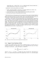
2.2.1. Compliance and Resonances of Lumped Mass Systems

Any one of the building blocks of an AFM, be it the body of the microscope itself or the force measuring
cantilevers, is a mechanical resonator. These resonances can be excited either by the surroundings or by
the rapid movement of the tip or the sample. To avoid problems due to building or air-induced oscilla-
tions, it is of paramount importance to optimize the design of the scanning probe microscopes for high
resonance frequencies; which usually means decreasing the size of the microscope (Pohl, 1986). By using
cubelike or spherelike structures for the microscope, one can considerably increase the lowest eigenfre-
quency. The eigenfrequency of any spring is given by
(2.3)

where

k

is the spring constant and

m

eff

is the effective mass. The spring constant

k

of a cantilevered beam
with uniform cross section is given by (Thomson, 1988)
(2.4)
where

E

is the Young’s modulus of the material, l

the length of the beam, and

I

the moment of inertia.
For a rectangular cross section with a width

b

(perpendicular to the deflection) and a height

h,

one
obtains for

I

(2.5)
k
m
=ω
2
2
k
m
=






h
h
ω
2

2
f
k
m
=
π
1
2
eff
k
EI
=
3
3
l
,
I
bh
=
3
12

© 1999 by CRC Press LLC

Combining Equations 2.3 through 2.5, and we get the final result for f :
(2.6)
The effective mass can be calculated using Rayleigh’s method. The general formula using Rayleigh’s
method for the kinetic energy

T of a bar is

(2.7)
For the case of a uniform beam with a constant cross section and length

L,

one obtains for the deflection

z

(

x

) =

z

max

(1 – (3

x)

/(2 l

) + (

x

3

)/(2l

3

). Inserting

z

max

into Equation 2.7 and solving the integral gives
(2.8)
and
for the effective mass.
Combining Equations 2.4 and 2.8 and noting that

m

=

ρl bh , where

ρ is the density of mass, one
obtains for the eigenfrequency
(2.9)
Further reading on how to derive this equation can be found in the literature (Thomson, 1988). It
is evident from Equation 2.9, that one way to increase the eigenfrequency is to choose a material
with as high a ratio

E /

ρ

. Another way to increase the lowest eigenfrequency is also evident in
Equation 2.9. By optimizing the ratio
h /l
2
one can increase the resonance frequency. However, it
does not help to make the length of the structure smaller than the width or height. Their roles will
just be interchanged. Hence, the optimum structure is a cube. This leads to the design rule, that
long, thin structures like sheet metal should be avoided. For a given resonance frequency the quality
factor should be as low as possible. This means that an inelastic medium such as rubber should be
in contact with the structure to convert kinetic energy into heat.

2.2.2 Cantilevers

Cantilevers are mechanical devices specially shaped to measure tiny forces. The analysis given in the
previous chapter is applicable. However, to understand better the intricacies of force detection systems
we will discuss the example of a straight cantilevered beam (Figure 2.1).
f
EI
m
Ebh
m
=
π
=
π
1

2
3
1
2
4
3
3
3
ll
eff eff
T
m
x
dx=
∂
()
∂








∫
1
2
0
2

l
l
z
t
T
m
zx
t
xx
dx
mzt
=
∂
()
∂
−






+















=
()
∫
ll
l
l
0
3
3
2
1
3
2
1
2
max
maxeff
m
eff
m=
9
20
f

Eh
=
π








1
2
5
3 ρ
l
2

© 1999 by CRC Press LLC

The bending of beams with a cross section

A

(

x

) is governed by the Euler equation (Thomson, 1988):
(2.10)

where

E

is Young’s modulus,

I

(

x

) the flexure moment of inertia defined by
(2.11)
Equations 2.10 and 2.11 can be derived by evaluating torsion moments about an element of infinites-
imal length at position

x

.
Figure 2.2 shows the forces and moments acting on an element of the beam.

V

is the shear moment,

M

the bending moment, and

p

(

x

) the position-dependent load per unit length. Summing forces in the

z

-direction, one obtains
(2.12)
Summing moments on the right face of the element gives
(2.13)
Finally, one obtains for the shear and bending moments
(2.14)

FIGURE 2.1 A

typical force microscope cantilever with a
length l

, a width

b

, and a height

h

. The height of the tip is

a

.
The material is characterized by Young’s modulus

E

, the shear
modulus

G

=

E

/(2(1 +

σ

)), where

σ

is the Poisson number,
and a density

ρ

.

FIGURE 2.2

Moments and forces acting on an
element of the beam.
d
dx
EI x
d
dx
zpx
2
2
2
2
()






=
()
I x z dydz
Ax
()
=

()
∫
2
dV p x dx−
()
= 0
dM Vdx p x dx−−
()( )
=
1
2
2
0
dV
dx
px
dM
dx
V
=
()
=
© 1999 by CRC Press LLC
Combining both parts of Equation 2.14, one obtains the following result
(2.15)
Using the flexure equation to express the bending moment, one obtains
(2.16)
Combining Equations 2.15 and 2.16, and one obtains the Euler Equation 2.10. Beams with a nonuni-
form cross section are difficult to calculate. Let us, therefore, concentrate on straight beams. These
cantilever beams are widely used for friction mode as well as for noncontact experiments.

A force acting on the cantilever at a position x
0
can be handled by the Dirac function δ(x – x
0
), for
which one has
(2.17)
Hence, one sets
(2.18)
where l is the length of the cantilever. Integrating M twice from the beginning to the end of the cantilever,
one obtains
(2.19)
since the moment must vanish at the end point of the cantilever. Integrating twice more and observing
that EI is a constant for beams with an uniform cross section, one gets
(2.20)
The slope of the beam is
(2.21)
Evaluating this and Equation 2.20 at the end of the cantilever, i.e., for x = l, one gets
(2.22)
dM
dx
dV
dx
px
2
2
==
()
MEI
dz

dx
=
2
2
fx x x dx fx
()
−
()
=
()
−∞
∞
∫
δ
00
px F
()
=
()
δ l
Mx xF
()
=−
()
l
dz
dx
Mx
EI
zx

EI
xx
F
2
2
3
2
6
3
=
()
⇒
()
=






−






l
ll
′

()
== −






=−






zx
dz
dx EI
xx
F
x
EI
x
F
l
ll
l
l
2
2

2
2
2
z
EI
F
z
EI
F
z
l
l
l
l
l
l
()
=−
′
()
=− =
()
3
2
3
2
3
2
© 1999 by CRC Press LLC
z′(l) is also the tangent of the deflection angle. Using the definition of the moment of inertia for a beam

with a rectangular cross section,
(2.23)
where b is the width and h the thickness of the lever, one gets for the deformation z at the end of the
cantilever is related to the applied normal force F by
(2.24)
Hence, the compliance k
N
is
(2.25)
and a change in angular orientation of the end of
(2.26)
We can ask ourselves what will, to first order, happen if we apply a lateral force F
L
to the end of the
cantilever. The cantilever will bend sideways and it will twist. The sideways bending can be calculated
with Equation 2.24 by exchanging b and h
(2.27)
Therefore, the compliance for bending in lateral direction is larger than the compliance for bending in
the normal direction by (b/h)
2
. The twisting or torsion on the other side is more complicated to handle.
For wide, thin cantilevers (b ӷ h), we obtain
(2.28)
The ratio of the torsion compliance to the bending compliance is (Colchero, 1993)
(2.29)
where we assumed a Poisson ratio s = 0.333. We see that thin, wide cantilevers with long tips favor torsion
while cantilevers with square cross sections and short tips favor bending. Finally, we calculate the ratio
between the torsion compliance and the normal mode-bending compliance.
(2.30)
Ibh=

1
12
3
z
Eb h
F=






4
3
l
k
F
z
Eb h
N
==






4
3
l

∆
∆
α=






=
63
2
2
Ebh h
F
z
N
l
l
k
F
z
Eh b
Lb
L
,
==







∆ 4
3
l
k
Gbh
a
L,tor
=
3
2
3l
k
k
ab
h
L
Lb
,
,
tor
=







1
2
2
l
k
ka
L
N
,tor
=






2
2
l
© 1999 by CRC Press LLC
Equations 2.28 to 2.30 hold in the case where the cantilever tip is exactly in the middle axis of the
cantilever. Triangular cantilevers and cantilevers with tips not on the middle axis can be dealt with by
finite-element methods.
The third possible deflection mode is the one from the forces along the cantilever axis. Their effect
on the cantilever is a torque. The boundary condition for the free end of the cantilever is M
0
= a*F
Fr
(see
Figure 2.3). This leads to the following modification of Equation 2.19:

(2.31)
Integration of Equation 2.31 now leads to
(2.32)
A second integration gives the deflection
(2.33)
Evaluating Equations 2.32 and 2.33 at the end of the cantilever, we get the deflection and the tilt due to
the normal force F
N
and the force from the front F
Fr
(2.34)
These equations can be inverted. One obtains the two:
(2.35)
FIGURE 2.3 The effect of normal F
N
and frontal forces F
Fr
on a cantilever.
Mx xF Fa
N
()
=−
()
+l
Fr
′
()
== −







+








zx
dz
dx EI
xx
F axF
N
1
2
2
l
l
Fr
zx
EI
x
x
FaxF

N
()
=−






+








1
23
1
22
l
l
Fr
z
EI
F
a
EI

F
EI
a
FF
z
EI
F
a
EI
F
EI
aF F
NN
NN
l
lll l
l
llll
()
=− + = −






′
()
=− + = −







322
2
32 23
22
Fr Fr
Fr Fr
F
EI
z
z
F
EI
a
zz
N
Fr
=−
()
−
′
()









=−
()
−
′
()
()
12
2
2
32
3
2
l
l
ll
l
lll
© 1999 by CRC Press LLC
A second class of interesting properties of cantilevers is their resonance behavior. For cantilevered beams
one can calculate that the resonance frequencies are (Colchero, 1993)
(2.36)
with λ
0
= (0.596864 …)π, λ
1
= (1.494175 …)π, λ

n
→ (n + ½)π.
A similar Equation 2.36 as holds for cantilevers in rigid contact with the surface. Since there is an
additional restriction on the movement of the cantilever, namely, the location of its end point, the
resonance frequency increases. Only the λ
n
’s terms change to (Colchero, 1993)
with λ′
0
= (1.2498763…)π, λ′
1
= (2.2499997…)π, λ′
n
→ (n + ¼)π(2.37)
The ratio of the fundamental resonance frequency in contact to the fundamental resonance frequency
not in contact is 4.3851. For the torsion mode, we can calculate the resonance frequency to
(2.38)
for thin, wide cantilevers. In contact, we obtain
(2.39)
The amplitude of the thermally induced vibration can be calculated from the resonance frequency using
(2.40)
where k
b
is Boltzmann’s factor and k the compliance of the cantilever. Since force microscope cantilevers
are resonant structures, sometimes with rather high qualities Q, the thermal noise is not evenly distributed
as Equation 2.40 suggests. The spectral noise density below the peak of the response curve is
(2.41)
2.2.3 Tips and Cantilevers
The key to the successful operation of an AFM is the measurement of the interaction forces between the
tip and the sample surface. The tip would ideally consist of only one atom, which is brought in the

vicinity of the sample surface. The interaction forces between the AFM tip and the sample surface must
be smaller than about 10
–7
N for bulk materials and preferably well below 10
–9
N for organic macromol-
ecules. To obtain a measurable deflection larger than the inevitable thermal drifts and noise the cantilever
deflection for static measurements should be at least 10 nm. Hence, the spring constants should be less
than 10 N/m for bulk materials and less than 1 N/m for organic macromolecules. Experience shows that
cantilevers with spring constants of about 0.01 N/m work best in liquid environments, whereas stiffer
cantilevers excel in resonant detection methods.
ω
λ
ρ
n
n
hE
free
=
2
2
23
l
ω
ρ
0
2
tors
=π
h

b
G
l
ω
ω
0
0
2
132
tors,contact
tors
=
+
()
ab
∆z
kT
k
B
therm
=
z
kT
kQ
B
0
0
4
=
ω

in m Hz
© 1999 by CRC Press LLC
Building vibrations usually have frequencies in the range from 10 to 100 Hz. These vibrations are
coupled to the cantilever. To get an estimate, we use Equation 2.3. Inserting 100 Hz for the resonance
frequency and a spring constant of 0.1 N/m, we obtain an upper limit of the lumped effective mass m
eff
of 0.25 mg. The quality factor of this resonance in air is typically between 10 and 100. To get a reasonable
suppression of the excitation of cantilever oscillations, the resonance frequency of the cantilever has to
be at least a factor of 10 higher than the highest of the building vibration frequencies. This means, that
m
eff
has to be under any circumstances no larger than 0.25 mg/100 = 2.5 µg. It would be preferable to
limit the mass to 0.1 µg. This lumped mass m
eff
, however, is smaller than the real mass m, by a factor
that depends on the geometry of the cantilever.
A good rule of thumb says that the effective mass m
eff
is 9/20 of the real mass. Today, micro-machined
cantilevers are commercially available and are used almost exclusively.
2.2.4 Materials and Geometry
Cantilevers have been made from a whole range of materials (Pitsch et al., 1989; Akamine et al., 1990;
Grütter et al., 1990; Wolter et al., 1991; Colchero, 1993). Most common are cantilevers made of Si and
of Si
3
N
4
. As has been shown in Equation 2.25, Young’s modulus E and the density ρ are the material
parameters determining the resonance frequency, besides the geometry. The realizable thickness depends
on the fabrication process and the material properties. Grown materials such as Si

3
N
4
can be made thinner
than those fabricated out of the bulk.
The first row of Table 2.1 shows the different materials. The second row gives Young’s modulus. The
third row is the hardness, a quantity that is important to judge the durability of the cantilevers. The last
row, finally, shows the speed of sound, indicative of the resonance frequency for a given shape.
Cantilevers come basically in two shapes (Figure 2.4). Straight types are preferentially used for lateral
force measurements and noncontact modes. Their properties are rather easy to calculate. Triangular-
shaped cantilevers are easier to align. They are mostly made of silicon nitride. Their response to lateral
forces is more complicated.
Whereas type b must be calculated using finite-element methods, one can get a good estimate of the
normal force compliance of type c in Figure 2.4 using analytical methods. Using Equation 2.25 and
observing that the length of the two joined cantilever beams are l
2
eff
= l
2
+ (w/2)
2
, where w is the width
of the base of the cantilever, one gets for the compliance:
(2.42)
TABLE 2.1 Material Properties of Cantilevers
Diamond Si
3
N
4
Si W Ir Steel Au Al PMMA

E in GPa 1,000 300/180 110 410 530 200 80 70 2.5-3
Mohs Hardness 10 9 7 6 6–6.5 5–8.5 2.5–3 2–3 <1
c
long
in m/s 17,500 10,000 5,970 5,400 4,860 6,000 3,240 6,420 1,600
FIGURE 2.4 Shapes of cantilevers: (a) is preferentially used
for lateral force measurements and for noncontact measure-
ments; (b) and (c) are two types, mostly fabricated from
silicon nitride.
k
Ebh w
N
=+






3
2
2
32
24
l
© 1999 by CRC Press LLC
2.2.5 Outline of Fabrication
Most force sensors in use today or commercially available are manufactured either from silicon or
from silicon nitride. These two material systems are compatible with standard integrated circuit
processing techniques. The shape and the thickness are easily controlled with sub-100 nm precision.

This is necessary because the largest extension of the cantilevers is typically smaller than 300 µm.
Microfabrication techniques and batch processing are important prerequisites for any successful large-
scale production of force sensors.
The first published production recipe for cantilevers (Akamine et al., 1990) was for a sensor made of
silicon nitride. All silicon nitride levers available today are made more or less along the guidelines outlined
there. A silicon (100) wafer is thinned. Next, the tips are defined by masking the topside of the wafer
with oxide, leaving square openings with about 4-µm-long sides. They have to be oriented parallel to the
(110) directions. The silicon in these openings is attacked by the anisotropic etchant KOH. The etch
process is fastest parallel to the (111) surfaces. Therefore, a pyramidal-shaped depression is etched away.
Since the anisotropy of the etch rate is of the order of 100, the process slows down considerably once all
the sides of the pyramid meet. The etch process is then terminated.
In the next step the silicon nitride is grown on top of the silicon, on the side with the etch pits. The
thickness of the layer, together with the shape of the cantilever, determines the resonance frequency and
the compliance. Since the silicon nitride is grown, one has a very good control on the layer thickness.
Typically, cantilevers are 300 nm thick, or more. Calculated and experimentally verified spring constants
are of the order of 0.01 to 1 N/m. In a next step, Pyrex glass with openings for the cantilevers is bonded
from the topside onto the wafer. The remaining silicon is dissolved, leaving the cantilevers free. In the
last manufacturing step the cantilevers are coated with a thin reflective film, since most microscopes use
light reflected off the back of the cantilever to detect its deflection. Gold is usually used as the coating
material, together with a 1-nm layer of chromium as an adhesion layer.
The radius of curvature of silicon nitride cantilevers is limited to about 30 to 50 nm, because of the
manufacturing process. The imperfections of the etch pits and the filled-in silicon nitride limit the
sharpness. Silicon nitride tips can be sharpened during the production by thermal oxidation (Akamine
and Quate, 1992). Instead of directly depositing silicon nitride on the wafers with the pyramidal etch
pits, an oxide layer is deposited first. Then, the silicon nitride is added. When the oxide was removed
with buffered oxide etch, a sharpening effect was observed. Details of the process are described by the
inventors (Akamine and Quate, 1992). A second method is to grow in an electron microscope a so-called
supertip on top of the silicon nitride. It is well known that in scanning electron microscopes with a base
pressure of more than 10
–10

mbar hydrocarbon residues are present. These residues are cracked at the
surface of the sample by the electron beam, leaving carbon in a presumed amorphous state on the surface.
It is known that prolonged imaging in such an instrument degrades the surface. If the electron beam is
not scanned, but stays at the same place, one can build up tips with a diameter comparable with the
electron beam diameter and with a height determined by the dwell time. These tips are extremely sharp;
they can reach radii of curvature of a few nanometers. They allow therefore an imaging with a very high
resolution. In addition, they enable the microscope to image the bottoms of small crevasses and ditches
on samples. Unprocessed silicon nitride tips are not able to do this, since their sides enclose an angle of
90°, due to the crystal structure of the silicon.
Silicon nitride cantilevers are less expensive than those made of other materials. They are very rugged
and well suited to imaging in almost all environments. They are especially compatible to organic and
biological materials.
Alternatives to silicon nitride cantilevers are those made of silicon. The basic manufacturing idea is
the same as for silicon nitride. Masks determine the shape of the cantilevers. Processes from the
microelectronics fabrication are used. Since the thickness of the cantilevers is determined by etching
and not by growth, wafers have to be more precise as for the manufacturing of the silicon nitride
cantilevers.
© 1999 by CRC Press LLC
The first step in the process is a wet chemical etch to thin the wafer to a thin membrane (Wolter et al.,
1991; Kassing and Oesterschulze, 1997). The membrane thickness is adjusted such that it corresponds
to the lever thickness and the tip height (10 to 30 µm). The resulting membrane must be free of stresses.
The next step is to define the cantilever layout by reactive ion etching and by chemical etching, which
already creates freestanding cantilevers, as used later on in the microscopes. The third step is to define
the tip. One way starts with a small oxide cap at the place where the tip should be. The silicon is then
attacked by KOH. Its anisotropical etching characteristics then attack the silicon such that the protective
oxide cap is underetched. The art of cantilever manufacturing consists in timing this process such that
the silicon under the tip is just about to be etched away. The caps then fall down, and the rupture site
produces cantilevers with well-defined radii of curvature of 2 to 5 nm. An example of such a cantilever
is shown in Figure 2.5. The end section of the cantilever is shown. The lever is rounded to minimize
unwanted contacts of the lever edge with the sample. Improved fabrication processes have made it possible

to produce regularly tips with a radius of curvature of 2 nm. Tips, such as the one shown in Figure 2.6,
permit imaging at the highest resolution in all known imaging modes.
Since the thickness of the cantilever is determined by etching, it cannot be made as thin as in the
silicon nitride case. The lower limit is typically 1 µm. Therefore, the stiffness of the silicon cantilevers is
higher, ranging from 1 to 100 N/m. Since the material is a single crystal, unlike the silicon nitride, it has
a very high quality of the resonance. Values exceeding 100,000 have been observed in vacuum. Therefore,
silicon cantilevers are often used for noncontact or tapping mode experiments. The cantilevers have two
drawbacks when working in the contact mode. First, they have a very high affinity to organic materials.
They often destroy such samples. Second, their index of refraction matches the one of water rather closely.
Silicon cantilevers have a very poor reflectivity in aqueous environments.
There are efforts under way to make cantilevers of GaAs (Kassing and Oesterschulze, 1997). This
material is more difficult to process, but it would offer new advantages. GaAs is a direct band gap material.
Optoelectronic functions could be easily integrated into such cantilevers. The investigation of magnetic
properties could be improved by the use of spin-polarized tunneling.
Occasionally, cantilevers are made with tungsten wire or thin metal foils, with tips of diamond or
other materials glued to it.
FIGURE 2.5 A commercial cantilever from Nanosensors. (Courtesy of Nanosensors.)
© 1999 by CRC Press LLC
2.3 Optical Detection Systems
2.3.1 Interferometer
Soon after the first papers on the AFM (Binnig et al., 1986), which used a tunneling sensor, an instrument
based on an interferometer was published (McClelland et al., 1987). The sensitivity of the interferometer
depends on the wavelength of the light employed in the apparatus. Figure 2.7 shows the principle of such
an interferometric design. The light incident from the left is focused by a lens on the cantilever. The
FIGURE 2.6 A SuperSharpSilicon™ tip from Nanosensors. The distance between two points on the scale in the
image is 18 nm. (Courtesy of Nanosensors. Used with permission.)
FIGURE 2.7 Principle of an interferometric AFM. The light of the laser light source is polarized by the polarizing
beam splitter and focused on the back of the cantilever. The light passes twice through a quarter wave plate and is
hence orthogonally polarized to the incident light. The second arm of the interferometer is formed by the flat. The
interference pattern is modulated by the oscillating cantilever.

© 1999 by CRC Press LLC
reflected light is collimated by the same lens and interferes with the light reflected at the flat. To separate
the reflected light from the incident light, a λ/4-plate converts the linear polarized incident light to
circular polarization. The reflected light is made linear polarized again by the λ/4-plate, but with a
polarization orthogonal to that of the incident light. The polarizing beam splitter then deflects the
reflected light to the photodiode.
2.3.1.1 Homodyne Interferometer
To improve the signal-to-noise ratio of the interferometer, the lever is driven by a piezoactuator near its
resonance frequency. The amplitude ∆z of the lever is
(2.43)
where ∆z
0
is the constant drive amplitude, Ω
0
the resonance frequency of the lever, Q the quality of the
resonance, and Ω the drive frequency. The resonance frequency of the lever is given by the effective
potential
(2.44)
where k is the spring constant of the free lever, U the interaction potential between the tip and the sample,
and m
eff
the effective mass of the cantilever. Equation 2.44 shows that an attractive potential decreases
the resonance frequency Ω
0
. The change in the resonance frequency Ω
0
in turn results in a change of the
lever amplitude ∆z (see Equation 2.43).
The movement of the cantilever changes the path difference in the interferometer. The light reflected
from the lever with the amplitude A

l,0
and the reference light with the amplitude A
r,0
interfere on the
detector. The detected intensity I(t) = {A
l
(t) + A
r
(t)}
2
consists of two constant terms and a fluctuating
term:
(2.45)
Here ω is the frequency of the light, δ the path difference in the interferometer, and ∆z is the instantaneous
amplitude of the lever, given according to Equations 2.43 and 2.44 as a function of the driving frequency
Ω, the spring constant k, and the interaction potential U. The time average of Equation 2.45 then becomes
(2.46)
Here all small quantities have been omitted and functions with small arguments have been linearized.
The amplitude of the lever oscillation ∆z can be recovered with a lock-in technique. However,
Equation 2.46 shows that the measured amplitude is also a function of the path difference δ in the
∆Ω ∆
Ω
ΩΩ
ΩΩ
zz
Q
()
=
−
()

+
0
0
2
2
0
2
2
2
0
2
2
Ω
0
2
2
1
=+
∂
∂






k
U
z
m

eff
2
44
00
AtAt AA t
z
tt
lr lr
() ()
=+
π
+
π
()






()
,,
sin sin sinω
δ
λλ
ω
∆
Ω
2
44

44
44
AtAt
z
t
z
t
z
t
lr
T
() ()
∝
π
+
π
()








≈
π







−
π
()








≈
π






−
π
()
cos sin
cos sin sin
cos sin
δ
λλ

δ
λλ
δ
λλ
∆
Ω
∆
Ω
∆
Ω
© 1999 by CRC Press LLC
interferometer. Hence, this path difference δ must be very stable. The best sensitivity is obtained when
sin(4δ/λ) ≈ 0.
2.3.1.2 Heterodyne Interferometer
This influence is not present in the heterodyne detection scheme shown in Figure 2.8. Light incident
from the left with a frequency ω is split in a reference path (upper path in Figure 2.8) and a measurement
path. Light in the measurement path is shifted in frequency to ω
1
= ω + ∆ω and focused on the cantilever.
The cantilever oscillates at the frequency Ω, as in the homodyne detection scheme. The reflected light
A
l
(t) is collimated by the same lens and interferes on the photodiode with the reference light A
r
(t). The
fluctuating term of the intensity is given by
(2.47)
where the variables are defined as in Equation 2.45. Setting the path difference sin(4πδ/λ) ≈ 0 and taking
the time average, omitting small quantities and linearizing functions with small arguments, we get
(2.48)

FIGURE 2.8 Heterodyne interferometer AFM. Light with the frequency ω
0
is split into a reference path (upper
path) and a measurement path. The light in the measurement path is frequency shifted to ω
1
by an acousto-optical
modulator (or an electro-optical modulator). The light reflected from the oscillating cantilever interferes with the
reference beam on the detector.
2
44
00
AtAt A A t
z
tt
lr lr
() ()
=+
()
+
π
+
π
()






()

,,
sin sin sinωω
δ
λλ
ω∆
∆
Ω
2
44
44
44
4
AtAt t
z
t
t
z
t
t
z
t
tr
T
() ()
∝+
π
+
π
()







=+
π






π
()






−+
π






π

()






≈
π





cos sin
cos cos sin
sin sin sin
cos
∆
∆
Ω
∆
∆
Ω
∆
∆
Ω
ω
δ
λλ

ω
δ
λλ
ω
δ
λλ
δ
λ

−
π
()






≈+
π






−
π
()







sin sin
cos sin
4
4
1
8
22
2
∆
Ω
∆
∆
Ω
z
t
t
z
t
λ
ω
δ
λ
λ
© 1999 by CRC Press LLC
Multiplying electronically the components oscillating at ∆ω and ∆ω + Ω and rejecting any product except

the one oscillating at Ω, we obtain
(2.49)
Unlike in the homodyne detection scheme, the recovered signal is independent from the path difference
δ of the interferometer. Furthermore, a lock-in amplifier with the reference set sin(∆ωt) can measure
the path difference δ independent of the cantilever oscillation. If necessary, a feedback circuit can keep
δ = 0.
2.3.1.3 Fiber-Optic Interferometer
The fiber-optic interferometer (Rugar et al., 1989) is one of the simplest interferometers to build and
use. Its principle is sketched in Figure 2.9. The light of a laser is fed into an optical fiber. Laser diodes
with integrated fiber pigtails are convenient light sources. The light is split in a fiber-optic beam splitter
into two fibers. One fiber is terminated by an index-matching oil to avoid any reflections back into the
fiber. The end of the other fiber is brought close to the cantilever in the AFM. The emerging light is
partially reflected back into the fiber by the cantilever. Most of the light, however, is lost. This is not a
−
ππ






()
=+
π







−
π
+
π
sin sin
cos cos
44
48 4
22
2
∆
∆Ω
∆
∆
∆
z
tt
t
z
t
λ
ω
δ
λ
ω
δ
λ
λ
ω
δ

λ






()
−
π
+
π






()
=+
π






−
π
+

π






−
π
+
π






()
−
π
sin
sin sin
cos cos
cos cos
sin
Ω
∆
∆Ω
∆
∆

∆
∆
∆Ω
∆
∆
t
z
tt
t
z
t
z
tt
z
44
44 4
44
2
4
22
2
22
2
λ
ω
δ
λ
ω
δ
λ

λ
ω
δ
λ
λ
ω
δ
λ
λ
ωω
δ
λ
ω
δ
λ
λ
λ
ω
δ
λ
ω
δ
λ
tt
t
z
z
tt
+
π







()
=+
π






−
π






+
π
+
()
+
π









+−
()
+
π


















+

4
4
1
4
2
2
4
2
4
2
22
2
22
2
sin
cos
cos cos
Ω
∆
∆
∆
∆Ω ∆Ω
ππ
+
()
+
π









+−
()
+
π


















∆
∆Ω ∆Ω
z

tt
λ
ω
δ
λ
ω
δ
λ
cos cos
44
A
zz
tt
zz
tt
z
t
=−
π






+
()
+
π







+
π






=−
π






+
()
+
π







+
()






≈
π
2
1
4
2
44
1
4
2
8
22
2
22
2
∆∆
∆Ω ∆
∆∆
∆Ω Ω
∆
Ω

λ
λ
ω
δ
λ
ω
δ
λ
λ
λ
ω
δ
λ
λ
cos cos
cos cos
cos
(()
© 1999 by CRC Press LLC
big problem since only 4% of the light is reflected at the end of the fiber, at the glass–air interface. The
two reflected light waves interfere with each other. The product is guided back into the fiber coupler and
again split into two parts. One half is analyzed by the photodiode. The other half is fed back into the
laser. Communications-grade laser diodes are sufficiently resistant against feedback to be operated in
this environment. They have, however, a bad coherence length, which in this case does not matter, since
the optical path difference is in any case no larger than 5 µm. Again, the end of the fiber has to be
positioned on a piezo drive to set the distance between the fiber and the cantilever to λ (n + ¼).
2.3.1.4 Nomarski Interferometer
Another solution to minimize the optical path difference uses the Nomarski (Schönenberger and Alva-
rado, 1989). Figure 2.10 depicts a sketch of the microscope. The light of a laser is focused on the cantilever
by a lens. A birefringent crystal (for instance, calcite) between the cantilever and the lens with its optical

axis 45° off the polarization direction of the light splits the light beam into two paths, offset by a distance
given by the length of the birefringent crystal. Birefringent crystals have varying indexes of refraction. In
calcite, one crystal axis has a lower index than the other two. This means that certain light rays will
propagate at a different speed through the crystal than others. By choosing a correct polarization, one
can select the ordinary ray, the extraordinary ray, or one can get any distribution of the intensity among
those two rays. A detailed description of birefringence can be found in textbooks (Shen, 1984). A calcite
crystal deflects the extraordinary ray at an angle of 6° within the crystal. By choosing a suitable length
of the calcite crystal, any separation can be set.
FIGURE 2.9 A typical setup for a fiber-optic interferometer readout.
FIGURE 2.10 Principle of the Nomarski AFM (Schönenberger and Alvarado, 1989, 1990). The circular polarized
input beam is deflected to the left by a nonpolarizing beam splitter. The light is focused onto a cantilever. The calcite
crystal between the lens and the cantilever splits the circular polarized light into two spatially separated beams with
orthogonal polarizations. The two light beams reflected from the lever are superimposed by the calcite crystal and
collected by the lens. The resulting beam is again circular polarized. A Wollaston prism produces two interfering
beams with a π/2 phase shift between them. The minimal path difference accounts for the excellent stability of this
microscope.
© 1999 by CRC Press LLC
The focus of one light ray is positioned near the free end of the cantilever while the other is placed
close to the clamped end. Both arms of the interferometer pass through the same space, except for the
distance between the calcite crystal and the lever. The closer the calcite crystal is placed to the lever, the
less influence disturbances like air currents have.
2.3.2 Sensitivity
Sarid (1991) has given values for the sensitivity of the different interferometeric detection systems.
Table 2.2 shows a summary of his results.
2.4 Optical Lever
The most common cantilever deflection detection system is the optical lever (Meyer and Amer, 1988;
Alexander et al., 1989). This method, depicted in Figure 2.11, employs the same technique as light beam
deflection galvanometers. A fairly well collimated light beam is reflected off a mirror and projected to a
receiving target. Any change in the angular position of the mirror will change the position where the
light ray hits the target. Galvanometers use optical path lengths of several meters and scales projected to

the target wall as a readout help.
For the AFM using the optical lever method, a photodiode segmented into two (or four) closely spaced
devices detects the orientation of the end of the cantilever (see Figure 2.11). Initially, the light ray is set
to hit the photodiodes in the middle of the two subdiodes. Any deflection of the cantilever will cause an
imbalance of the number of photons reaching the two halves. Hence, the electrical currents in the
TABLE 2.2 Noise in Interferometers
Homodyne
Interferometer,
Fiber-Optic
Interferometer
Heterodyne
Interferometer
Nomarski
Interferometer
Laser noise 〈δi
2
〉
L
Thermal noise 〈δi
2
〉
l
Shot noise 〈δi
2
〉
S
4eηP
d
B 2eη(P
R

+ P
S
)B
F is the finesse of the cavity in the homodyne interferometer, P
i
is the incident power, P
d
is the
power on the detector, η is the sensitivity of the photodetector, and RIN is the relative intensity noise
of the laser. P
R
and P
S
are the power in the reference and sample beam in the heterodyne interferometer.
P is the power in the Nomarsky interferometer, and δΘ is the phase difference between the reference
and the probe beam in the Nomarsk y interferometer. B is the bandwidth and e the electron charge.
λ is the wavelength of the laser and k the stiffness of the cantilever, T is the temperature.
FIGURE 2.11 Optical lever setup.
1
4
222
η FP
i
RIN
η
22 2
PP
RS
+
()

RIN
1
16
22
ηδP Θ
16
4
2
2
222
0
π
λ
η
ω
FP
k TBQ
k
i
B
4
4
2
2
22
0
π
λ
η
ω

P
k TBQ
k
d
B
π
λ
η
ω
2
2
22
0
4
P
k TBQ
k
B
1
2
ePBη
© 1999 by CRC Press LLC
photodiodes will be unbalanced, too. The difference signal is further amplified and is the input signal to
the feedback loop. Unlike the interferometric AFMs, where often a modulation technique is necessary
to get a sufficient signal-to-noise ratio, most AFMs employing the optical lever method are operated in
a static mode. AFMs based on the optical lever method are universally used. It is the simplest method
to construct an optical readout and it can be confined in volumes smaller than 5 cm on the side.
The optical lever detection system is a simple yet elegant way to detect normal and lateral force signals
simultaneously (Meyer and Amer, 1988, 1990; Alexander et al., 1989; Marti, Colchero et al., 1990). It has
the additional advantage that it is a remote detection system.

2.4.1 Implementations
Light from a laser diode or from a superluminescent diode is focused on the end of the cantilever. The
reflected light is directed onto a quadrant diode that measures the direction of the light beam. A Gaussian
light beam far from its waist is characterized by an opening angle β. The deflection of the light beam by
the cantilever surface tilted by an angle α is 2α. The intensity on the detector then shifts to the side by
the product of 2α and the separation between the detector and the cantilever. The readout electronics
calculates the difference of the photocurrents. The photocurrents, in turn, are proportional to the intensity
incident on the diode.
The output signal is hence proportional to the change in intensity on the segments:
(2.50)
Figure 2.12 shows a schematic drawing of the optical lever setup. For the sake of simplicity, we assume
that the light beam is of uniform intensity with its cross section increasing proportionally with the
distance between the cantilever and the quadrant detector. The movement of the center of the light beam
is then given by
(2.51)
The photocurrent generated in a photodiode is proportional to the number of incoming photons hitting
it. If the light beam contains a total number of N
0
photons, then the change in difference current becomes
(2.52)
FIGURE 2.12 The setup of optical lever detection microscope.
II
sig tot
∝ 4
α
β
∆∆xz
d
Det
=

l
∆∆∆I I I zdN
RL
−
()
==const
0
© 1999 by CRC Press LLC
Combining Equations 2.51 and 2.52, one obtains that the difference current ∆I is independent of the
separation of the quadrant detector and the cantilever. This relation is true if the light spot is smaller
than the quadrant detector. If it is greater, the difference current ∆I becomes smaller with increasing
distance. In reality, the light beam has a Gaussian intensity profile. For small movements ∆x (compared
with the diameter of the light spot at the quadrant detector), Equation 2.52 still holds. Larger movements
∆x, however, will introduce a nonlinear response. If the AFM is operated in a constant-force mode, only
small movements ∆x of the light spot will occur. The feedback loop will cancel out all other movements.
The scanning of a sample with an AFM can twist the microfabricated cantilevers because of lateral
forces (Mate et al., 1987; Marti et al., 1990; Meyer and Amer, 1990) and affect the images (den Boef,
1991). When the tip is subjected to lateral forces, it will twist the lever, and the light beam reflected from
the end of the lever will be deflected perpendicular to the ordinary deflection direction. For many
investigations, this influence of lateral forces is unwanted. The design of the triangular cantilevers stems
from the desire to minimize the torsion effects. However, lateral forces open up a new dimension in force
measurements. They allow, for instance, a distinction of two materials because of the different friction
coefficient, or the determination of adhesion energies. To measure lateral forces the original optical lever
AFM has to be modified; Figure 2.13 shows a sketch of the instrument. The only modification compared
with Figure 2.12 is the use of a quadrant detector photodiode instead of a two-segment photodiode and
the necessary readout electronics. The electronics calculates the following signals:
(2.53)
The calculation of the lateral force as a function of the deflection angle does not have a simple solution
for cross sections other than circles. An approximate formula for the angle of twist for rectangular beams
is (Baumeister and Marks, 1967)

(2.54)
FIGURE 2.13 Scanning force and friction microscope (SFFM). The lateral forces exerted on the tip by the moving
sample cause a torsion of the lever. The light reflected from the lever is deflected orthogonally to the deflection caused
by normal forces.
UIIII
UIIII
Normal Force Upper Left Upper Right Lower Left Lower Right
Lateral Force Upper Left Upper Left Lower Right Lower Right
=+
()
−+
()
[]
=+
()
−+
()
[]
α
β
Θ=
M
Gb h
t
l
β
3
© 1999 by CRC Press LLC
where M
t

= Fa is the external twisting moment due to friction, l is the length of the beam, b and h the
sides of the cross section, G the shear modulus, and β a constant determined by the value of h/b. For the
equation to hold, h has to be larger than b.
Inserting the values for a typical microfabricated lever with integrated tips
(2.55)
into Equation 2.54, we obtain the relation
(2.56)
Typical lateral forces are of order 10
–10
N.
2.4.2 Sensitivity
The sensitivity of this setup has been calculated in various papers (Colchero et al., 1991; Sarid, 1991;
Colchero, 1993), to name just three examples. Assuming a Gaussian beam, the resulting output signal as
a function of the deflection angle is dispersion like. Equation 2.50 shows that the sensitivity can be
increased by increasing the intensity of the light beam I
tot
or by decreasing the divergence of the laser
beam. The upper bound of the intensity of the light I
tot
is given by saturation effects on the photodiode.
If we decrease the divergence of a laser beam, we automatically increase the beam waist. If the beam waist
becomes larger than the width of the cantilever, we start to get diffraction. Diffraction sets a lower bound
on the divergence angle. Hence, one can calculate the optimal beam waist w
opt
and the optimal divergence
angle β (Colchero et al., 1991; Colchero, 1993)
(2.57)
where b is the width of the cantilever and λ is the wavelength of the light. The optimal sensitivity of the
optical lever then becomes
(2.58)

The angular sensitivity optical lever can be measured by introducing a parallel plate into the beam. A
tilt of the parallel plate results in a displacement of the beam, mimicking an angular deflection.
Additional noise source can be considered. Of little importance is the quantum mechanical uncertainty
of the position (Colchero et al., 1991; Colchero, 1993), which is for typical cantilevers at room temperature
b =×
×
×
−
610
7
m
h =10 m
=10 m
a = 3.3 10 m
G=5 10 Pa
= 0.333
-5
-4
-6
10
l
β
FN
Lateral Force
=× ×
−
11 10
4
. Θ
wb

b
opt
opt
≈
≈
036
089
.
.θ
λ
ε
λ
mW rad mW
tot
[]
=
[]
18.
b
I
© 1999 by CRC Press LLC
(2.59)
At very low temperatures and for high-frequency cantilevers, this could become the dominant noise
source. A second noise source is the shot noise of the light. The shot noise is related to the particle
number. We can calculate the number of photons incident on the detector
(2.60)
where I is the intensity of the light, τ the measurement time, B = 1/τ the bandwidth, c the speed of light,
and λ the wavelength of the light. The shot noise is proportional to the square root of the number of
particles. Equating the shot noise signal with the signal resulting for the deflection of the cantilever, one
obtains

(2.61)
where w is the diameter of the focal spot. Typical AFM setups have a shot noise of 2 pm. The thermal
noise can be calculated from the equipartition principle. The amplitude at the resonance frequency is
(2.62)
where Q is the quality of the cantilever resonance, ω
0
the resonance frequency, and k is the stiffness of
the cantilever spring. A typical value is 16 pm. Upon touching the surface, the cantilever increases its
resonance frequency by a factor of 4.39. This results in a new thermal noise amplitude of 3.2 pm for the
cantilever in contact with the sample.
2.5 Piezoresistive Detection
2.5.1 Implementations
An alternative detection system which is not as widespread as the optical detection schemes are piezore-
sistive cantilevers (Ashcroft and Mermin, 1976; Stahl et al., 1994; Kassing and Oesterschulze, 1997). These
levers are based on the fact that the resistivity of certain materials, in particular of Si, changes with the
applied stress. Figure 2.14 shows a typical implementation of a piezoresistive cantilever. Four resistances
are integrated on the chip, forming a Wheatstone bridge. Two of the resistors are in unstrained parts of
the cantilever; the other two are measuring the bending at the point of the maximal deflection. For
instance, when an AC voltage is applied between terminals A and C one can measure the detuning of
the bridge between terminals B and D. With such a connection, the output signal varies only due to bending,
but not due to changing of the ambient temperature and thus the coefficient of the piezoresistance.
2.5.2 Sensitivity
The resistance change is (Kassing and Oesterschulze, 1997)
(2.63)
∆z
m
==
h
2
005

0
ω
.fm
n
II
Bc
I
B
==
π
=×
[]
[]
τ
ω
λ
hh2
18 10
9
.
W
Hz
∆z
w
B
I
shot
kHz
mW
fm=

[]
[]
[]
68
l
∆z
B
kQ
therm
Nm
pm=
[]
[]
129
0
ω
∆R
R
0
=Πδ
© 1999 by CRC Press LLC
where ∏ is the tensor element of the piezoresistive coefficients, δ the mechanical stress tensor element,
and R
0
the equilibrium resistance. For a single resistor, they separate the mechanical stress and the tensor
element in longitudinal and transversal components.
(2.64)
The maximum value of the stress components are ∏
t
= –64.0 × 10

–11
m
2
/N and ∏
l
= 71.4 × 10
–11
m
2
/N
for a resistor oriented along the (110) direction in silicon (Kassing and Oesterschulze, 1997). In the
resistor arrangement of Figure 2.14 two of the resistors are subject to the longitudinal piezoresistive effect
and two of them are subject to the transversal piezoresistive effect. The sensitivity of that setup is about
four times that of a single resistor, with the advantage that temperature effects cancel to first order. It is
then calculated that
(2.65)
where the geometric constants are defined in Figure 2.1, F is the normal force applied to the end of the
cantilever, ∆z is the deflection resulting from this force, and ∏ = 67.7 × 10
–11
m
2
/N

is the averaged
piezoresistive coefficient. Plugging in typical values for the dimensions (ᐉ = 100 µm, b = 10 µm, h =
1 µm), one obtains that
(2.66)
The sensitivity can be tailored by optimizing the dimensions of the cantilever.
2.6 Capacitive Detection
The capacitance of an arrangement of conductors depends on the geometry. Generally speaking, the

capacitance increases for decreasing separations. Two parallel plates form a simple capacitor (see
Figure 2.15, upper left), with the capacitance
(2.67)
FIGURE 2.14 A typical setup for a piezoresistive readout.
∆R
R
tt ll
0
=Π +Πδδ
∆
∆
R
R
Eh
z
bh
F
0
22
3
2
6
=Π =Π
l
l
∆R
R
F
0
5

410
=
×
−
nN
C
A
x
=
εε
0
© 1999 by CRC Press LLC
where A is the area of the plates, assumed equal, and x the separation. Alternatively, one can consider a
sphere vs. an infinite plane (see Figure 2.15, lower left). Here, the capacitance is (Sarid, 1991)
(2.68)
where R is the radius of the sphere and α is defined by
(2.69)
One has to keep in mind that capacitance of a parallel plate capacitor is a nonlinear function of the
separation. Using a voltage divider, one can circumvent this problem.
Figure 2.16a shows a low-pass filter. The output voltage is given by
(2.70)
Here, C is given by Equation 2.67, ω is the excitation frequency, and j is the imaginary unit. The
approximate relation in the end is true when ωCR ӷ 1. This is equivalent to the statement that C is fed
by a current source, since R must be large in this setup. Plugging this equation into Equation 2.70 and
neglecting the phase information, one obtains
(2.71)
which is linear in the displacement x.
FIGURE 2.15 Three possible arrangements of a capacitive readout.
The upper left shows the cross section through a parallel plate capac-
itor. The lower left shows the geometry sphere vs. the plane. The

right side shows the more-complicated, but linear capacitive readout.
FIGURE 2.16 Measuring the capacitance. The left side (a) shows a low-pass filter; the right side (b) shows a
capacitive divider. C (left) or C
2
are the capacitances under test.
CR
n
n
=π
()
()
=
∞
∑
4
0
2
ε
α
α
sinh
sinh
α=++ +









ln 1 2
2
2
z
R
z
R
z
R
UU
jC
R
jC
U
jCR
U
jCR
out
=
+
=
+
≅
≈≈
≈
1
1
1
1

ω
ω
ωω
U
Ux
RA
out
=
≈
ωεε
0