Tài liệu Handbook of Micro and Nano Tribology P11 docx

Harrison, J.A. et al. “Atomic-Scale Simulation of Tribological and Related ”
Handbook of Micro/Nanotribology.
Ed. Bharat Bhushan
Boca Raton: CRC Press LLC, 1999

© 1999 by CRC Press LLC

11

Atomic-Scale
Simulation of
Tribological and

Related Phenomena

Judith A. Harrison, Steven J. Stuart,
and Donald W. Brenner

11.1 Introduction
11.2 Molecular Dynamics Simulations

Interatomic Potentials • Thermodynamic Ensemble •
Temperature Regulation

11.3 Nanometer-Scale Material Properties: Indentation,
Cutting, and Adhesion

Indentation of Metals • Indentation of Metals Covered by
Thin Films • Indentation of Nonmetals • Cutting of
Metals • Adhesion

11.4 Lubrication at the Nanometer Scale: Behavior of
Thin Films

Equilibrium Properties of Confined Thin Films • Behavior of
Thin Films under Shear

11.5 Friction

Solid Lubrication • Friction in the Presence of a Third
Body • Tribochemistry

11.6 Summary
Acknowledgments
References

11.1 Introduction

Understanding and ultimately controlling friction and wear have long been recognized as important to
many areas of technology. Historical examples include the Egyptians, who had to invent new technologies
to move the stones needed to build the pyramids (Dowson, 1979); Coulomb, whose fundamental studies
of friction were motivated by the need to move ships easily and without wear from land into the water
(Dowson, 1979); and Johnson et al. (1971), whose study of automobile windshield wipers led to a better
understanding of contact mechanics, including surface energies. Today, the development of microscale

© 1999 by CRC Press LLC

(and soon nanoscale) machines continues to challenge our understanding of friction and wear at their
most fundamental levels.
Our knowledge of friction and related phenomena at the atomic scale has rapidly advanced over the
last decade with the development of new and powerful experimental methods. The surface force apparatus

(SFA), for example, has provided new information related to friction and lubrication for many liquid
and solid systems with unprecedented resolution (Israelachvili, 1992). The friction force and atomic force
microscopes (FFM and AFM) allow the frictional and mechanical properties of solids to be characterized
with atomic resolution under single-asperity contact conditions (Binnig et al., 1986; Mate et al., 1987;
Germann et al., 1993; Carpick and Salmeron, 1997). Other techniques, such as the quartz crystal
microbalance, are also providing exciting new insights into the origin of friction (Krim et al., 1991; Krim,
1996). Taken together, the results of these studies have revolutionized the study of friction, wear, and
mechanical properties, and have reshaped many of our ideas about the fundamental origins of friction.
Concomitant with the development and use of these innovative experimental techniques has been the
development of new theoretical methods and models. These include analytic models, large-scale molec-
ular dynamics (MD) simulations, and even first-principles total-energy techniques (Zhong and Tomanek,
1990). Analytic models have had a long history in the study of friction. Beginning with the work of
Tomlinson (1929) and Frenkel and Kontorova (1938), through to recent studies by McClelland and Glosli
(1992), Sokoloff (1984, 1990, 1992, 1993, 1996), and others (Helman et al., 1994; Persson, 1991), these
idealized models have been able to break down the complicated motions that create friction into basic
components defined by quantities such as spring constants, the curvature and magnitude of potential
wells, and bulk phonon frequencies. The main drawback of these approaches is that simplifying assump-
tions must be made as part of these models. This means, for example, that unanticipated defect structures
may be overlooked, which may strongly influence friction and wear even at the atomic level.
Molecular dynamics computer simulations, which are the topic of this chapter, represents a compro-
mise between analytic models and experiment. On the one hand, this method deals with approximate
interatomic forces and classical dynamics (as opposed to quantum dynamics), so it has much in common
with analytic models (for a comparison of analytic and simulation results, see Harrison et al., 1992c).
On the other hand, simulations often reveal unanticipated events that require further analysis, so they
also have much in common with experiment. Furthermore, a poor choice of simulation conditions, as
in an experiment, can result in meaningless results. Because of this danger, a thorough understanding
of the strengths and weaknesses of MD simulations is crucial to both successfully implementing this
method and understanding the results of others.
On the surface, atomistic computer simulations appear rather straightforward to carry out: given a
set of initial conditions and a way of describing interatomic forces, one simply integrates classical

equations of motion using one of several standard methods (Gear, 1971). Results are then obtained from
the simulations through mathematical analysis of relative positions, velocities, and forces; by visual
inspection of the trajectories through animated movies; or through a combination of both (Figure 11.1).
However, the effective use of this method requires an understanding of many details not apparent in this
simple analysis. To provide a feeling for the details that have contributed to the success of this approach
in the study of adhesion, friction, and wear as well as other related areas, the next section provides a
brief review of MD techniques. For a more detailed overview of MD simulations, including computer
algorithms, the reader is referred to a number of other more comprehensive sources (Hoover, 1986;
Heermann, 1986; Allen and Tildesley, 1987; Haile, 1992).
The remainder of this chapter presents recent results from MD simulations dealing with various aspects
of mechanical, frictional, and wear properties of solid surfaces and thin lubricating films. Section 11.2
summarizes several of the technical details needed to perform (or understand) an MD simulation. These
range from choosing an interaction potential and thermodynamic ensemble to implementing tempera-
ture controls. Section 11.3 describes simulations of the indentation of metals and nonmetals, as well as
the machining of metal surfaces. The simulations discussed reveal a number of interesting phenomena
and trends related to the deformation and disordering of materials at the atomic scale, some (but not
all) of which have been observed at the macroscopic scale. Section 11.4 summarizes the results of

© 1999 by CRC Press LLC

simulations that probe the properties of liquid films confined to thicknesses on the order of atomic
dimensions. These systems are becoming more important as demands for lubricating moving parts
approach the nanometer scale. In these systems, fluids have a range of new properties that bear little
resemblance to liquid properties on macroscopic scales. In many cases, the information obtained from
these studies could not have been obtained in any other way, and is providing unique new insights into
recent observations made by instruments such as the SFA. Section 11.5 discusses simulations of the
tribological properties of solid surfaces. Some of the systems discussed are sliding diamond interfaces,
Langmuir–Blodgett films, self-assembled monolayers, and metals. The details of several unique mecha-
nisms of energy dissipation are discussed, providing just a few examples of the many ways in which the
conversion of work into heat leads to friction in weakly adhering systems. In addition, simulations of

molecules trapped between, or chemisorbed onto, diamond surfaces will be discussed in terms of their
effects on the friction, wear, and tribology of diamond. A summary of the MD results is given in the
final section.

11.2 Molecular Dynamics Simulations

Atomistic computer simulations are having a major impact in many areas of the chemical, physical,
material, and biological sciences. This is largely due to enormous recent increases in computer power,

FIGURE 11.1

Flow chart of an MD simulation.

© 1999 by CRC Press LLC

increasingly clever algorithms, and recent developments in modeling interatomic interactions. This last
development, in particular, has made it possible to study a wide range of systems and processes using
large-scale MD simulations. Consequently, this section begins with a review of the interatomic interac-
tions that have played the largest role in friction, indentation, and related simulations. For a slightly
broader discussion, the reader is referred to a review by Brenner and Garrison (1989). This is followed
by a brief discussion of thermodynamic ensembles and their use in different types of simulations. The
section then closes with a description of several of the thermostatting techniques used to regulate the
temperature during an MD simulation. This topic is particularly relevant for tribological simulations
because friction and indentation do work on the system, raising its kinetic energy.

11.2.1 Interatomic Potentials

Molecular dynamics simulations involve tracking the motion of atoms and molecules as a function of
time. Typically, this motion is calculated by the numerical solution of a set of coupled differential
equations (Gear, 1971; Heermann, 1986; Allen and Tildesley, 1987). For example, Newton’s equation of

motion,
(11.1)
where

F

is the force on a particle,

m

is its mass,

a

its acceleration,

v

its velocity, and

t

is time, yield a set
of 3

n

(where

n

is the number of particles) second-order differential equations that govern the dynamics.
These can be solved with finite-time-step integration methods, where time steps are on the order of

1

/

25

of a vibrational frequency (typically tenths to a few femtoseconds) (Gear, 1971). Most current simulations
then integrate for a total time of picoseconds to nanoseconds. The evaluation of these equations (or any
of the other forms of classical equations of motion) requires a method for obtaining the force

F

between
atoms.
Constraints on computer time generally require that the evaluation of interatomic forces not be
computationally intensive. Currently, there are two approaches that are widely used. In the first, one
assumes that the potential energy of the atoms can be represented as a function of their relative atomic
positions. These functions are typically based on simplified interpretations of more general quantum
mechanical principles, as discussed below, and usually contain some number of free parameters. The
parameters are then chosen to closely reproduce some set of physical properties of the system of interest,
and the forces are obtained by taking the gradient of the potential energy with respect to atomic positions.
While this may sound straightforward, there are many intricacies involved in developing a useful potential
energy function. For example, the parameters entering the potential energy function are usually deter-
mined by a limited set of known system properties. A consequence of that is that other properties,
including those that might be key in determining the outcome of a given simulation, are determined
solely by the assumed functional form. For a metal, the properties to which a potential energy function

might be fit might include the lattice constant, cohesive energy, elastic constants, and vacancy formation
energy. Predicted properties might then include surface reconstructions, energetics of interstitial defects,
and response (both elastic and plastic) to an applied load. The form of the potential is therefore crucial
if the simulation is to have sufficient predictive power to be useful.
The second approach, which has become more useful with the advent of powerful computers, is the
calculation of interatomic forces directly from first-principles (Car and Parrinello, 1985) or semiempirical
(Menon and Allen, 1986; Sankey and Allen, 1986) calculations that explicitly include electrons. The
advantage of this approach is that the number of unknown parameters may be kept small, and, because
the forces are based on quantum principles, they may have strong predictive properties. However, this
does not guarantee that forces from a semiempirical electronic structure calculation are accurate; poorly
chosen parameterizations and functional forms can still yield nonphysical results. The disadvantage of
this approach is that the potentials involved are considerably more complicated, and require more
computational effort, than those used in the classical approach. Longer simulation times require that
Fa
v
==mm
d
dt
,

© 1999 by CRC Press LLC

both the system size and the timescale studied be smaller than when using more approximate methods.
Thus, while this approach has been used to study the forces responsible for friction (Zhong and Tomanek,
1990), it has not yet found widespread application for the type of large-scale modeling discussed here.
The simplest approach for developing a continuous potential energy function is to assume that the
binding energy

E

b

can be written as a sum over pairs of atoms,
(11.2)
The indexes

i

and

j

are atom labels,

r

ij

is the scalar distance between atoms

i

and

j,

and

V

pair

(

r

ij

) is an
assumed functional form for the energy. Some traditional forms for the pair term are given by
(11.3)
where the parameter

D

determines the minimum energy for pairs of atoms. Two common forms of this
expression are the Morse potential (

X

=

e

–

β

r
ij

), and the Lennard–Jones (LJ) “12-6” potential (

X

= (

σ

/

r

ij

)

6

).
(

β

and

σ

are arbitrary parameters that are used to fit the potential to observed properties.)
The short-range exponential form for the Morse function provides a reasonable description of repulsive

forces between atomic cores, while the 1/

r

6

term of the LJ potential describes the leading term in long-
range dispersion forces. A compromise between these two is the “exponential-6,” or Buckingham, poten-
tial. This uses an exponential function of atomic distances for the repulsion and a 1/

r

6

form for the
attraction. The disadvantage of this form is that as the atomic separation approaches zero, the potential
becomes infinitely attractive.
For systems with significant Coulomb interactions, the approach that is usually taken is to assign each
atom a fractional point charge

q

i

. These point charges then interact with a pair potential
Because the 1/

r

Coulomb interactions act over distances that are long compared to atomic dimensions,

simulations that include them typically must include large numbers of atoms, and often require special
attention to boundary conditions (Ewald, 1921; Heyes, 1981).
Other forms of pair potentials have been explored, and each has its strengths and weaknesses. However,
the approximation of a pairwise-additive binding energy is so severe that in most cases no form of pair
potential will adequately describe every property of a given system (an exception might be rare gases).
This does not mean that pair potentials are without use — just the opposite is true! A great many general
principles of many-body dynamics have been gleaned from simulations that have used pair potentials,
and they will continue to find a central role in computer simulations. As discussed below, this is especially
true for simulations of the properties of confined fluids.
A logical extension of the pair potential is to assume that the binding energy can be written as a many-
body expansion of the relative positions of the atoms
(11.4)
Normally, it is assumed that this series converges rapidly so that four-body and higher terms can be
ignored. Several functional forms of this type have had considerable success in simulations. Stillinger
and Weber (1985), for example, introduced a potential of this type for silicon that has found widespread
EVr
bij
ji
i
=
()
>
()
∑∑
pair
.
Vr DXX
ijpair
()
=⋅ −

()
1,
Vr
qq
r
ij
ij
ij
pair
()
= .
EV V V
jikjilkji
b body body body
=+ + +…
−− −
∑∑∑∑∑∑∑∑∑
1
2
1
3
1
4
23 4
!!
.

© 1999 by CRC Press LLC

use, an example of which is discussed in Section 11.3.3. Another example is the work of Murrell and co-

workers (1984) who have developed a number of potentials of this type for different gas-phase and
condensed-phase systems.
A common form of the many-body expansion is a valence force field. In this approach, interatomic
interactions are modeled with a Taylor series expansion in bond lengths, bond angles, and torsional
angles. These force fields typically include some sort of nonbonded interaction as well. Prime examples
include the molecular mechanics potentials pioneered by Allinger and co-workers (Allinger et al., 1989;
Burkert and Allinger, 1982). A common variation of the valence-force approach is to assume rigid bonds,
and allow only changes in bond angles. Because the angle bends generally have smaller force constants,
there tend to be larger variations in angles than in bond lengths, so this approximation often gives accurate
predictions for the shapes of large molecules at thermal energies. The advantage of this approximation
is that because the bending modes have lower frequencies than those involving bond stretching modes,
time steps may be used that are an order of magnitude larger than those required for flexible bonds, with
no larger numerical errors in the total energy.
One method of including many-body effects in Coulomb systems is to account for electrostatic
induction interactions. Each point charge will give rise to an electric field, and will induce a dipole
moment on neighboring atoms. This effect can be modeled by including terms for the atomic or molecular
dipoles in the interaction potential, and solving for the values of the dipoles at each step in the dynamics
simulation. An alternative method is to simulate the polarizability of a molecule by allowing the values
of the point charges to change directly in response to their local environment (Streitz and Mintmire,
1994; Rick et al., 1994). The values of the charges in these simulations are determined by the method of
electronegativity equalization and may either by evaluated iteratively (Streitz and Mintmire, 1994) or
carried as dynamic variables in the simulation (Rick et al., 1994).
Several potential energy expressions beyond the many-body expansion have been successfully devel-
oped and are widely used in MD simulations. For metals, the embedded atom method (EAM) and related
methods have been highly successful in reproducing a host of properties, and have opened up a range
of phenomena to simulation (Finnis and Sinclair, 1984; Foiles et al., 1986; Ercollessi et al., 1986a,b). These
have been especially useful in simulations of the indentation of metals, as discussed in Section 11.3. This
approach is based on ideas originating from effective medium theory (Norskov and Lang, 1980; Stott
and Zaremba, 1980). In this formalism, the energy of an atom interacting with surrounding atoms is
approximated by the energy of the atom interacting with a homogeneous electron gas and a compensating

positive background. The EAM assumes that the density of the electron gas can be approximated by a
sum of electron densities from surrounding atoms, and adds a repulsive term to account for core–core
interactions. Within this set of approximations, the total binding energy is given as a sum over atomic sites
(11.5)
where each site energy is given as a pair sum plus a contribution from a functional (called an embedding
function) that, in turn, depends on the sum of electron densities at that site:
(11.6)
The function

Φ

(

r

ij

) represents the core–core repulsion,

F

is the embedding function, and

ρ

(

r

ij

) is the
contribution to the electron density at site

i

from atom

j

. For practical applications, functional forms are
assumed for the core–core repulsion, the embedding function, and the contribution of the electron
densities from surrounding atoms. For a more complete description of this approach, including a much
more formal derivation and discussion, the reader is referred to Sutton (1993).
EE
bi
i
=
∑
,
ErFr
iij
j
ij
j
=
()
+
()









∑∑
1
2
Φρ.

© 1999 by CRC Press LLC

For close-packed metals, it has been found that the electron densities in the solid can be adequately
approximated by a pairwise sum of atomic-like electron densities. With this approximation, the com-
puting time required to evaluate an EAM potential scales with the number of atoms in the same way as
a pair potential. The quantitative results of the EAM, however, are dramatically better than those obtained
with pair potentials. Energies and structures of solid surfaces and defects in metals, for example, match
experimental results (or more-sophisticated calculations) reasonably well despite the relatively simple
analytic form. Because of this, EAM potentials have been used extensively in studies of indentation.
Schemes similar to EAM but based on other levels of approximation have also been developed. For
example, three-body terms in the electron-density contributions have been studied for modeling a range
of metallic and covalently bonded systems (Baskes, 1992). Another example is the work of DePristo and
co-workers, who have studied various hierarchies of approximation within effective medium theory by
including additional correction terms to Equation 11.6 (Raeker and DePristo, 1991), as have Norskov
and co-workers (Jacobson et al., 1987).
A potential that is similar to the EAM but based on bond orders has also been developed (Abell, 1985).
Originally adapted by Tersoff (1986) to model silicon, the approach has found use in computer simula-
tions of a wide range of covalently bonded systems (Tersoff, 1989; Brenner, 1989a, 1990; Khor and Das

Sarma, 1988). Like the embedded atom potentials, Tersoff potentials begin by approximating the binding
energy of a system as a sum over sites:
(11.7)
In this case, however, each site energy is given by an expression that resembles a pair potential,
(11.8)
The functions

V

A

(

r

ij

) and

V

R

(

r

ij

) represent pairwise-additive attractive and repulsive terms, respectively,

and

B

ij

represents an empirical bond-order expression that modulates the attractive pair potential. This
bond-order term is where the many-body effects are introduced. As in the other potentials, functional
forms for the bond order and the pair terms are fit to a range of properties for the systems of interest.
Applications of this approach have assumed functional forms for the bond order that decrease its value
as the number of nearest-neighbors of a given pair of bonded atoms increases. Physically, the attractive
pair term can be envisioned as bonding due to valence electrons, with the bond order destabilizing the
bond as the valence electrons are shared among more and more neighbors. Tersoff, Abell, and others
have shown that this simple expression can capture a range of bond energies, bond lengths, and related
properties for group IV solids. Also, if properly parameterized, the potential yields Pauling’s bond-order
relations (Abell, 1985; Khor and Das Sarma, 1988; Tersoff, 1989). These properties have been shown to
make this expression very powerful for predicting covalently bonded structures and, therefore, useful for
predicting new phenomena through MD simulations.
Although they are based on different principles, the EAM and Tersoff expressions are quite similar. In
the EAM, binding energy is defined by electron densities through the embedding function. The electron
densities are, in turn, defined by the arrangement of neighboring atoms. Similarly, in the Tersoff expres-
sion the binding energy is defined directly by the number and arrangement of neighbors through the
bond-order expression. In fact, the EAM and Tersoff approaches have been shown to be identical for
simplified expressions provided that angular interactions are not used (Brenner, 1989b).
Although not all potential energy expressions widely used in MD simulations have been covered, this
section provides a brief introduction to those that have found the most use in the simulations of friction,
wear, and related phenomena. As mentioned above, methods that explicitly incorporate semiempirical
and first-principles electronic structure calculations have not been discussed. As computer speeds
EE
bi

i
=
∑
.
EVrBVr
i R ij ij A ij
ji
=
()
+⋅
()
[]
>
()
∑
.

© 1999 by CRC Press LLC

continue to increase and as new algorithms are developed, we expect that these more exact methods will
play an increasingly important role in tribological simulations.

11.2.2 Thermodynamic Ensemble

When performing a MD simulation, a choice must be made as to which thermodynamic ensemble to
study. These ensembles are distinguished by which thermodynamic variables are held constant over the
course of the simulation. (For a broader and more rigorous treatment of ensemble averaging, the reader
should consult any statistical mechanics text, (e.g., McQuarrie, 1976)).
Without specific reasons to do otherwise, it is quite natural to keep the number of atoms (

N

) and the
volume of the simulation cell (

V

) constant over the course of a MD simulation. In addition, for a system
without energy transfer, integrating the equations of motion (Equation 11.1) will generate a trajectory
over which the energy of the system (

E

) will also be conserved. A simulation of this type is thus performed
in the constant-

NVE,

or microcanonical, ensemble.
Systems undergoing sliding friction or indentation, however, require work to be performed on the
system, which raises its energy and causes the temperature to increase. In a macroscopic system, the
environment surrounding the region of tribological interest acts as an infinite heat sink, removing excess
energy and helping to maintain a fairly constant temperature. Ideally, a sufficiently large simulation would
be able to model this same behavior. But while the thousands of atoms at an atomic-scale interface are
within reach of computer simulation, the

O

(10

23

) atoms in the experimental apparatus are not. Thus, a
thermodynamic ensemble that will more closely resemble reality will be one in which the temperature
(

T

), rather than the energy, is held constant. These simulations are performed in the constant-

NVT,

or
canonical, ensemble.
A constant temperature is maintained in the canonical ensemble by using any of a large number of
thermostats, many of which are described in the following section. What is often done in simulations of
indentation or friction is to apply the thermostat only in a region of the simulation cell that is well
removed from the interface where friction is taking place. This allows for local heating of the interface
as work is done on the system, while also providing a means for efficient dissipation of excess heat. These
“hybrid”

NVE/NVT

simulations, although not rigorously a member of any true thermodynamic ensem-
ble, are very useful and quite common in tribological simulations.
A particularly troublesome system for MD simulations is the nonequilibrium dynamics of confined
thin films (see Section 11.4.2). In these systems, the constraint of constant atom number is not necessarily
applicable. Under experimental conditions, a thin film under shear or tension is free to exchange mole-
cules with a reservoir of bulk liquid molecules, and the total atom number is certainly conserved. But
the number of atoms in the film itself is subject to rather dramatic changes. According to some studies,

as many as half the molecules in an ultrathin film will exit the interfacial region upon a change in registry
of the opposing surfaces (i.e., with no change in interfacial volume) (Schoen et al., 1989). Changes in
the film particle number can be equally large under compression.
The proper conserved quantity in these simulations is not the particle number

N,

but the chemical
potential

µ

. During a simulation performed in the constant-

µ

VT,

or grand canonical, ensemble, the
number of atoms or molecules fluctuates to keep the chemical potential constant. A true grand canonical
MD simulation is too difficult to perform for all but the simplest of liquid molecules, however, due to
the difficulties associated with inserting or removing molecules at bulk densities. An alternative chosen
by some authors is to mimic the experimental reservoir of bulk liquid molecules on a microscopic scale.
This involves performing a constant-

NVT

(Wang et al., 1993a,b, 1994) or constant-

NPT

(Gao et al., 1997)
simulation that explicitly includes a collection of molecules that are external to the interfaces (see
Figure 11.14). As liquid molecules drain into or are drawn from the reservoir region, the number of
particles directly between the interfaces is free to change. This method is then an approximation to the
grand canonical ensemble when only a subset of the system is considered. Two drawbacks to this method
are that the interface can extend infinitely (via periodic boundary conditions) in only one dimension
instead of two, and also that a significant number of extraneous atoms must be carried in the simulation.

© 1999 by CRC Press LLC

An interesting alternative to the grand canonical ensemble is that chosen by Cushman and co-workers
(Schoen et al., 1989; Curry et al., 1994). They performed a series of grand canonical Monte Carlo
simulations at various points along a hypothetical sliding trajectory. These simulations were used to
calculate the correct particle numbers at a fixed chemical potential, which were in turn used as inputs
to nonsliding, constant-

NVE

MD simulations at each of the chosen trajectory points. Because the system
was fully equilibrated at each step along the sliding trajectory, the sliding speed can be assumed to be
infinitely slow. This offers a useful alternative to continuous MD simulations, which are currently
restricted to sliding speeds of roughly 1 m/s or greater — orders of magnitude larger than most experi-
mental studies.

11.2.3 Temperature Regulation

As was discussed in the previous section, some method of controlling the system temperature is required
in simulations involving friction or indentation. In this section, we discuss some of the many available
thermostats that are used for this purpose. For a more formal discussion of heat baths and the trajectories

that they produce, the reader is referred to Hoover (1986).
The most straightforward method for controlling heat production is simply to rescale intermittently
the atomic velocities to yield a desired temperature (Woodcock, 1971). This approach was widely used
in early MD simulations, and is often effective at maintaining a given temperature during the course of
a simulation. However, it has several disadvantages that have spurred the development of more-sophis-
ticated methods. First, there is little formal justification. For typical system sizes, averaged quantities,
such as pressure, do not correspond to those obtained from any particular thermodynamic ensemble.
Second, the dynamics produced are not time reversible, again making results difficult to analyze in terms
of thermodynamic ensembles. Finally, the rate and mode of heat dissipation are not determined by system
properties, but instead depend on how often velocities are rescaled. This may influence dynamics that
are unique to a particular system.
A more-sophisticated approach to maintaining a given temperature is through Langevin dynamics.
Originally used to describe Brownian motion, this method has found widespread use in MD simulations.
In this approach, additional terms are added to the equations of motion, corresponding to a frictional
term and a random force (Schneider and Stoll, 1978; Hoover, 1986; Kremer and Grest, 1990). The
equations of motion (see Equation 11.1) are given by
(11.9)
where

F

are the forces due to the interatomic potential, the quantities

m

and

v

are the particle mass and

velocity, respectively,

ξ

is a friction coefficient, and

R

(

t

) represents a random “white noise” force. The
friction kernel is defined in terms of a memory function in formal applications; kernels developed for
harmonic solids have been used successfully in MD simulations (Adelman and Doll, 1976; Adelman,
1980; Tully, 1980).
As with any thermostat, the atom velocities are altered in the process of controlling the temperature.
It is important to keep this in mind when using a thermostat, because it has the potential to perturb any
dynamic properties of the system being studied. To help avoid this problem, one effective approach is to
add Langevin forces only to those atoms in a region away from where the dynamics of interest occurs.
In this way, coupling to a heat bath is established away from the important action, and simplified
approximations for the friction term can be used without unduly influencing the dynamics produced by
the interatomic forces. For heat flux via nuclear (as opposed to electronic) degrees of freedom in solids,
it has been shown that a reasonable approximation for the friction coefficient

ξ

is 6/

π

times the Debye
frequency

β

(Adelman and Doll, 1976). Lucchese and Tully (1983) have shown that with this approxi-
mation and a sufficiently large reaction zone, the vibrational modes of atoms away from the bath atoms
are well described by the interatomic potential.
mmRtaF v== +
()
ξ ,

© 1999 by CRC Press LLC

The random force can be given by a Gaussian distribution where the width, which is chosen to satisfy
the fluctuation–dissipation theorem, is determined from the equation
(11.10)
The function

R

is the random force in Equation 11.9,

m

is the particle mass,

T

is the desired temperature,

k

is Boltzmann’s constant,

t

is time, and

ξ

is the friction coefficient. The random forces are uncoupled
from those at the previous steps (as denoted by the delta function), and the width of the Gaussian
distribution from which the random force is chosen depends on the temperature.
The simplified Langevin approach outlined above does not require any feedback from the current
temperature of the system; instead, the random forces are determined solely from Equation 11.10. A
slightly different expression has been developed that eliminates the random forces and replaces the
constant-friction coefficient with one that depends on the ratio of the desired temperature to current
kinetic energy of the system (measured as a temperature) (Berendsen et al., 1984). The resulting equations
of motion are
(11.11)
where

F

is the force due to the interatomic potential,

T

0

and

T

are the desired and actual temperatures,
respectively, and

v is again the particle velocity. The advantage of this approach is that it requires no
evaluation of random forces, which can be expensive for a large number of bath atoms. One disadvantage
in practice is that if the system is not pre-equilibrated to populate properly the vibrational modes, or if
nonrandom external forces are applied to the system, it can be slow to fully equilibrate the system. For
example, a simulated indentation of a solid surface requires that the bottom layers of the solid be held
rigid (Section 11.3). Compression of the surface during indentation may cause sound waves to propagate
into the bulk, reflect from the bottom layers, and continue to reflect between the surface and rigid layers.
Because the Berendsen thermostat uses a frictional force that depends on the average kinetic energy, it
would only reduce the total kinetic energy of the system, and not help dissipate a traveling wave. On the
other hand, the Langevin approach using a random force on each atom does not require feedback from
the system, and thermostats each atom individually. Thus, the random forces are much more efficient
in eliminating these nonphysical reflecting waves.
Nonequilibrium equations of motion have also been developed to maintain a constant temperature
(Hoover, 1986). Like the Berendsen thermostat, this approach adds a friction to the interatomic forces.
However, it is derived from Gauss’ principle of least constraint, which maintains that the sum of the
squares of any constraining forces on a system should be as small as possible. Using a Lagrange multiplier,
a frictional force on each atom i of the form
(11.12)
where
(11.13)
can be derived that maintains a constant temperature. The quantity m

i
is the mass of atom i, v
i
is its
velocity, and F
i
is the total force on atom i due to the interatomic potential. Note that there is no target
temperature in this expression; instead, the temperature of the system when the constraint is initiated is
R R t mkT t02
()
⋅
()
=
()
ξδ .
mm
T
T
aF v=+ −






ξ
0
1,
Fv
iii

m
friction
=−ς ,
ς= ⋅
()
()
∑∑
Fv v
ii
i
i
i
m
2
,
© 1999 by CRC Press LLC
maintained for all time. This approach has several obvious advantages. First, it does not rely on an
approximated input such as the Debye frequency as in the simplified Langevin or Berendsen thermostats.
Heat loss and gain are therefore determined only by implicit system properties. Second, because a random
force is not required, it does not significantly increase computational time. Third, the equations of motion
are time reversible. Finally, by differentiating total energy with respect to time, the heat loss (or gain)
due to the thermostat can be calculated directly (this is also true of the Langevin thermostat). However,
as with the Berendsen thermostat, coupling of the frictional to global properties of the system may be
slow to randomize nonphysical vibrational disturbances.
A thermostat that corresponds rigorously to a canonical ensemble has been developed by Nosé
(1984a,b). This significant advance also adds a friction term, but one that maintains the correct distri-
bution of vibrational modes. It achieves this by adding a new dimensionless variable to the standard
classical equations of motion that can be thought of as a large heat bath, which couples to each of the
physical degrees of freedom. The actual effect of the variable, however, is to scale the coordinates of either
time or mass in the system. The dynamics of the expanded system correspond to the microcanonical

ensemble, but when projected onto only the physical degrees of freedom they generate a trajectory in
the canonical ensemble. Sampling problems associated with very small or very stiff systems can be
overcome by attaching a series of these Nosé-Hoover thermostats to the system (Martyna et al., 1992).
The resulting equations of motion are time reversible, and the trajectories can be analyzed exactly with
well-established statistical mechanical principles (Martyna et al., 1992). For a complete description of
the Nosé thermostat, its relation to other formalisms for generating classical equations of motion, and
a comparison of the dynamics generated with this approach and the others that have been reviewed here,
the reader is referred to Hoover (1986).
Each of the potential energy functions, thermodynamic ensembles, and thermostats outlined above
has advantages and disadvantages. The optimum choice depends strongly on the particular system and
process being simulated as well as on the type of information in which one is interested. For example,
general principles related to liquid lubrication in confined areas may be most easily understood and
generalized from simulations that use pair potentials and may not require a thermostat. On the other
hand, if one wants to study the wear or indentation of a surface of a particular metal, then EAM or other
semiempirical potentials, together with a thermostat, may yield more reliable results. Even more-detailed
studies, including the evaluation of electronic degrees of freedom, may require interatomic forces derived
from some level of electronic structure calculation. The best way to make this choice is to understand
carefully the strong points of each of these approaches, decide what one wishes to learn from the
simulation, and form conclusions based on this careful understanding.
11.3 Nanometer-Scale Material Properties: Indentation,
Cutting, and Adhesion
Understanding material properties at the nanometer scale is crucial to developing the fundamental ideas
needed to design new coatings with tailor-made friction and wear properties. One of the ways in which
these properties is being characterized is through the use of the AFM. This technique is proving to be a
very versatile tool that can provide a rich variety of atomic-scale information pertaining to a given
tip–sample interaction (Burnham and Colton, 1993). For example, when an AFM tip (the radius of
curvature of AFM tips typically ranges from 100 Å to 100 µm) is rastered across a sample substrate and
the force on the tip perpendicular to the substrate is measured at each point, a force map of the surface
is obtained that can be related to the actual topography of the surface (Meyer et al., 1992). Rastering the
AFM tip across a substrate in the same way, but measuring the deflection of the tip in the lateral direction

instead, produces a friction map of the surface (Germann et al., 1993). Finally, by moving the tip
perpendicular to the surface of the substrate, the AFM can be used as a nanoindenter that probes the
mechanical properties of various substrates and thin films (Burnham and Colton, 1989; Burnham et al.,
1990).
© 1999 by CRC Press LLC
Adhesive contact can be examined by gradually moving the tip closer to the substrate until the two
come into contact. After contact, the tip is retracted from the surface, and any differences between the
force curves for contact and retraction reflect characteristics of adhesion. A plot of normal force on the
tip vs. tip–sample separation (i.e., a force curve) is typically made to record this sequence of events. A
force curve for the adhesive contact of a Ni tip with an Au substrate (denoted Ni/Au) is shown in
Figure 11.2a. This is a typical curve possessing the same qualitative features as most AFM force curves.
For instance, as the tip and the sample begin to interact, a small attractive well, due to long-range forces
(Burnham and Colton, 1993) is apparent in the force curve at large tip–sample separations (the well is
centered at a tip–sample separation of approximately 17 nm). The distance between the tip and the
sample is gradually decremented until the tip comes into contact with the sample. After contact the tip
is retracted, and adhesion between the tip and the substrate manifests itself as a hysteresis in the force
curve.
After contact, if the tip is moved farther toward the substrate, rather than away from the substrate,
indentation of the sample by the tip results. This indentation is reflected as a dramatic increase in force
as the tip is moved farther into the substrate (Figure 11.2b). This region of the force curve is known as
the repulsive wall region (Burnham and Colton, 1993), or when considered without the rest of the force
curve, an indentation curve. Retraction of the tip subsequent to indentation results in an enhanced
adhesion, therefore, in a larger hysteresis in the force curve. The origin of this enhanced adhesion is
discussed later.
Many types of adhesion at a tip–substrate interface are possible. Adhesion might result from the
formation of covalent chemical bonds between the tip and the sample. Alternatively, real surfaces usually
have a layer of liquid contamination on the surface that can lead to capillary formation and adhesion.
FIGURE 11.2 Experimentally measured force vs. tip-to-sample distance curves for an Ni tip interacting with an
Au substrate for contact followed by separation in (a) and contact, indentation, then separation in (b). These curves
were derived from AFM measurements taken in dry nitrogen. (From Landman, U. et al. (1990), Science 248, 454–461.

With permission.)
© 1999 by CRC Press LLC
In metallic systems a different sort of wetting is possible; specifically, the sample can be wet by the tip
(or vice versa). The result of this wetting is the formation of “connective neck” of metallic atoms between
the tip and the sample and a consequent adhesion. Finally, entanglement of molecules that are anchored
on the tip with molecules anchored on the sample could also be responsible for an observed hysteresis.
Molecular dynamics simulations of indentations were first employed in an effort to shed light on the
physical phenomena that are responsible for the qualitative shape of AFM force curves. In addition to
succeeding at this task, MD simulations have revealed an abundance of atomic-scale phenomena that
occur during the indentation process. In the remainder of this section, MD simulations related to
indentation and related processes are discussed.
11.3.1 Indentations of Metals
Landman et al. (1990) were among the first groups to use MD to simulate the indentation of a metallic
substrate with a metal tip. In an early simulation, a Ni tip was used to indent a Au(001) substrate. The
tip was originally arranged as a pyramid and contained 1400 dynamic atoms and 1176 rigid atoms used
as a holder. The substrate was composed of 11 layers of Au atoms containing 450 atoms each. These
constant-temperature simulations were carried out at 300 K. The forces governing the interatomic motion
of the system were derived from EAM potentials for Ni and Au.
After equilibration of the tip and substrate to 300 K, the tip was brought into contact with surface by
moving the tip holder 0.25 Å closer to the surface every 1525 fs. This rate (or a tip velocity of approximately
16 m/s), while fast compared with experiment, is much smaller than the speed of sound in Au, and
allowed the system to evolve dynamically such that only natural fluctuations of system properties
occurred. This process was continued throughout the indentation. By calculating the force on the rigid
layers of the tip while moving the tip closer to the sample, a plot of force vs. tip sample separation was
generated (Figure 11.3).
The shape of the computer-generated force curve for the indentation of the Au substrate by the Ni tip
showed qualitative agreement with the experimentally derived force curve (Figure 11.2b) with two
exceptions. First, there was no attractive well at large tip–sample separations in the computer-generated
force curve. This was due to the lack of long-range attractive interactions, such as dispersion forces, in
the simulations. Second, the computer-generated force curve contained a fine structure not present in

the force curve generated from experimental data.
FIGURE 11.3 Computationally derived force F
z
vs. tip-to-sample distance d
hs
curves for approach, contact, inden-
tation, then separation using the same tip–sample pair as in Figure 11.2. These data were calculated from an MD
simulation. (From Landman U. et al. (1990), Science 248, 454–461. With permission.)
© 1999 by CRC Press LLC
One advantage of simulations is that the shape of the force curve, along with its fine structure, can be
related to specific atomic-scale events. For instance, Landman et al. (1990) reported the observation of
a jump to contact (JC) that corresponded to that region of the force curve where there was a precipitous
drop in the force just prior to tip–substrate contact (Figure 11.3, point D). The JC phenomenon was
previously observed by Pethica and Sutton (1988) and by Smith et al. (1989). In this region of the force
curve, the gold atoms “bulged up” to meet the tip. Deformation occurred in the gold substrate because
its modulus is much lower than that of the nickel tip. This deformation occurred in a short time span
(approximately 1 ps) and was accompanied by wetting of the Ni tip by several Au atoms. Landman et al.
(1990) concluded that the JC phenomenon in metallic systems is driven by the tendency of the interfacial
atoms of the tip and the substrate to optimize their embedding energies while maintaining their individual
material cohesive binding.
Advancing the tip past the JC point caused indentation of the gold substrate accompanied by the
characteristic increase in force with decreasing tip–substrate separation (Figure 11.3, points D to M).
This region of the computer generated force curve had a maximum not present in the force curve
generated from experimental data (Figure 11.3, point L). The origin of this variation in force was tip-
induced flow of the Au atoms. This flow caused “piling-up” of Au atoms around the edges of the Ni
indenter. *
The force curve was completed by reversal of the tip motion (Figure 11.3, points M to X). The hysteresis
in this force curve was due to adhesion between the tip and the substrate. As the tip was retracted from
the sample, a “connective neck” of atoms between the tip and the substrate formed (Figure 11.4). While
this connective neck of atoms was largely composed of Au atoms, some Ni atoms did diffuse into the

neck. Retraction of the tip caused the magnitude of the force to increase (i.e., become more negative)
until, at some critical force, the atoms in adjacent layers of the connective neck rearranged so that an
FIGURE 11.4 Illustration of atoms in the MD simulation of an Ni tip being pulled back from an Au substrate.
This causes the formation of a connective neck of atoms between the tip and the surface. Red spheres represent Ni
atoms. The first layer of Au substrate is colored yellow, the second blue, the third green, the fourth yellow, and so
on. (From Landman U. et al. (1990), Science 248, 454–461. With permission.)*
* Color reproduction follows page 16.
© 1999 by CRC Press LLC
additional row of atoms formed in the neck. These rearrangement events were the essence of the
elongation process, and they were responsible for the fine structure (apparent as a series of maxima)
present in the retraction portion of the force curve. These elongation and rearrangement steps were
repeated until the connective neck of atoms was severed.
When the Ni tip was coated with an epitaxial gold monolayer (Landman et al., 1992) and the inden-
tation of an Au(001) substrate repeated, the adhesive contact between the tip and the substrate was
reduced. The JC instability, formation of an adhesive contact, and hysteresis during subsequent retraction
were all observed. In contrast to the Ni/Au study, complete separation of the tip and substrate resulted
in the transfer of a smaller number of substrate atoms to the tip when the connective neck of atoms,
composed entirely of Au, was severed. Because the tip was covered with Au, the interaction between the
tip and the substrate was composed mostly of Au–Au interactions, and Au possesses less of a tendency
to wet itself than it does to wet Ni. This accounted for the insignificant number of substrate atoms
transferred to the tip.
When a hard Ni tip indented a soft Au substrate, the substrate sustained most of the damage. Con-
versely, damage was predominately done to the tip when a soft tip was used to indent a hard substrate.
For example, Landman and Luedtke (1991) used a pyramidal Au(001) tip to indent a Ni(001) substrate.
These constant-temperature indentations were carried out in the same manner described above for the
Ni/Au system. Force curves generated from the indentation of the Ni substrate by the Au tip had the
same qualitative shape as the Ni/Au force curves. However, there were differences in the fine structure
of these force curves, therefore, in the atomic-scale events responsible for this structure. For instance, in
this case the tip bulged toward the substrate during the JC, rather than the substrate bulging toward the
tip. Thus, the softer material (i.e., the one with the lower modulus) was displaced during the JC. The

adhesive contact between the tip and the substrate caused large structural rearrangements in the interfacial
region of the Au tip. The closest three or four Au layers to the Ni substrate exhibited a marked tendency
toward a (111) reconstruction, consistent with an increase in interlayer spacing. In fact, this reconstruc-
tion persisted throughout the separation process.
When the tip was pushed farther toward the substrate subsequent to the JC, it became flattened (or
compressed) increasing its contact area. This flattening involved structural rearrangements of the outer
layers of the tip that reduced the number of crystalline layers, leaving an interstitial-layer defect in the
core of the tip. The interstitial defect was annealed away upon further compression of the tip. Upon
separation, a connective neck of Au atoms was formed due to adhesion between the Au and the Ni. This
connective neck of atoms underwent a series of elongation events, as in the Ni/Au study, until the
tip–sample distance was such that the neck became thin and broke.
Other metallic tip–substrate systems were examined with interesting results. For instance, Tomagnini
et al. (1993) studied the interaction of a pyramidal Au tip with a Pb(110) substrate using MD. These
constant-energy simulations were carried out at approximately room temperature and again at temper-
atures high enough to initiate surface melting of the Pb substrate (600 K). The forces were calculated
using a many-body potential, called the glue model, that is very similar to the EAM potentials (Ercolessi
et al., 1988).
At room temperature (300 K), when the Au tip was brought into close proximity to the Pb substrate,
a JC was initiated by a few Pb atoms wetting the Au tip. The connective neck of atoms between the tip
and the surface was composed almost entirely of Pb. The tip became deformed because the inner-tip
atoms were pulled more toward the sample surface than toward atoms on the tip surface. Because these
were constant-energy simulations, the energy released due to the wetting of the tip caused an increase
in temperature of the tip (of approximately 15 K). Extensive structural rearrangements in the tip occurred
when the tip–sample distance was decremented further. Results for the retraction of the tip from the Pb
substrate were not reported.
Increasing the substrate temperature to 600 K caused the formation of a liquid Pb layer (approximately
four layers thick) on the surface of the substrate. During the indentation, the distance at which the JC
occurred increased by approximately 1.5 Å. Due to the high diffusivity of Pb surface atoms at this
temperature, the contact area also increased. Eventually, the Au tip dissolved in the liquid Pb atom “bath.”
© 1999 by CRC Press LLC

This liquid-like connective neck of atoms followed the tip upon retraction. As a result, the liquid–solid
interface moved farther back into the bulk Pb substrate, increasing the length of the connective neck.
Similar elongation events have been observed experimentally. For example, scanning tunneling micros-
copy (STM) experiments on the same surface demonstrated that the neck can elongate approximately
2500 Å without breaking.
Similar atomic-scale phenomena were observed for an Ir tip indenting a Pb substrate (Raffi-Tabar
et al., 1992). These constant-temperature MD simulations made use of long-range, many-body Finnis-
Sinclair potentials formulated to model the interatomic forces between atoms in face-centered-cubic (fcc)
metallic alloys (Raffi-Tabar and Sutton, 1991). The method developed by Nosé (1984a) was used to
regulate the temperature of the simulation. This simulation was unique in that periodic boundary
conditions were also employed in the indentation direction. Therefore, images of the substrate–tip system
were located in the cells above and below the computational cell. Indentation of the substrate by the tip
was achieved by decrementing the computational cell length normal to the substrate surface.
During the indentation process, the Pb substrate wetted the Ir tip subsequent to the JC. Significant
structural rearrangement of the Pb substrate was brought about when the tip was pushed closer to the
substrate after the JC. This structural rearrangement led to a “piling up” of the Pb atoms around the
edges of the tip and was brought about by the local diffusional flow of the Pb atoms in much the same
way as it was when an Ni tip was used to indent a soft Au substrate (Landman et al., 1990). In both the
Ni/Au and the Ir/Pb systems, the tip (Ni and Ir) retained most of its shape because it was harder than
the substrate. Plastic flow in the Ir/Pb system resulted in a hysteresis in the force curve upon retraction
of the tip. The nonmonotonic features in the force curves generated from the Ir/Pb simulation were
associated with discrete, local, atomic movements; however, the precise nature of these movements was
not elucidated.
The large-scale indentation of approximately 70,000-atom Cu and Ag(111) surfaces with a rigid,
triangular-shaped tip has been simulated by Belak and co-workers (Belak and Stowers, 1992; Belak et al.,
1993). The forces between metal atoms in these large-scale MD simulations were derived from EAM
potentials and interaction between the tip and the metal substrate was modeled by an LJ potential.
Indentations were performed by moving the tip closer to the substrate at constant velocities of 1, 10, and
100 m/s. A Nosé thermostat (1984a) was used to control the temperature of the simulation.
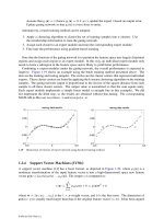
For the 1 m/s indentation of Cu(111), the load increased linearly with indentation depth until the tip

indented approximately 0.6 nm into the substrate (Figure 11.5). At this point, the surface yielded plas-
tically and the force dropped suddenly. This plastic yielding was concomitant with a single atom “pop-
ping” out onto the surface of the substrate from beneath the tip. Continued indentation caused several
of these events to occur. At the maximum indentation depth (1.7 nm) atoms from the substrate were
“piled up” around the edges of the tip (Figure 11.6) and plastic deformation was limited to a few lattice
spacings surrounding the tip. The piling up of atoms is typical in cases where a hard tip is used to indent
FIGURE 11.5 Computationally derived load vs. indentation
depth curve for the indentation of Cu(111) with a rigid tip.
These data were calculated from an MD simulation. (From
Belak, J. and Stowers, I. F. (1992), in Fundamentals of Friction:
Macroscopic and Microscopic Processes (I. L. Singer and H. M.
Pollock, eds.), 511–520, Kluwer, Dordrecht. With permission.)
© 1999 by CRC Press LLC
a soft substrate. Retracting the tip from the substrate caused the load to drop quickly to zero with only
small oscillations, presumably due to some plastic events at the surface. Both the pile up of substrate
atoms and the plastic nature of the indentation were apparent from analysis of the Cu(111) substrate
subsequent to indentation (Figure 11.6).
Plastic deformation in this system during the 1 m/s indentation occurred via the motion of point
defects. The formation of defects or dislocations was driven by the need to release stored elastic energy.
Plots of the energy required to create a dislocation and the elastic energy vs. length of the radius of the
indenter cross at length values of a few nanometers. In contrast, at the faster indentation rates of 10 m/s,
the system did not have time to relax completely and the stored elastic energy was much greater.
Eventually, the surface yielded and a small dislocation loop was observed on the surface.
Even though the tip was much sharper for the indentation of the Ag(111), the force curves generated
from that indentation were similar to those generated from the indentation of Cu(111). For the 1 m/s
indentation, the initial plastic events corresponded to the “popping” of single atoms out of the substrate.
The hardness value obtained from this simulation, estimated from the load divided by contact area, was
approximately 4 GPa, or approximately four times larger than the experimentally determined hardness
value of approximately 1 GPa (Pharr and Oliver, 1989).
11.3.2 Indentation of Metals Covered by Thin Films

Using simulation procedures similar to those in their earlier work, Raffi-Tabar and Kawazoe (1993) used
an Ir tip to indent an Ir substrate that was covered with a monolayer Pb film. As the tip approached the
Pb/Ir substrate, the Pb atoms directly below the tip strained upward to wet the Ir tip and a JC was
observed. The disruption of the Pb monolayer caused by the JC also resulted in local deformation of the
Ir substrate beneath the monolayer. Further indentation resulted in penetration of the Pb film at only
FIGURE 11.6 Illustration of Cu(111) substrate atoms in an MD simulation after indentation by a rigid tip at 1 m/s.
The piling-up of the substrate atoms (gray spheres) around the edge of the tool tip after indentation is evident in
this picture. (From Belak, J. and Stowers, I. F. (1992), in Fundamentals of Friction: Macroscopic and Microscopic
Processes (I. L. Singer and H. M. Pollock, eds.), 511–520, Kluwer, Dordrecht. With permission.)
© 1999 by CRC Press LLC
one atomic site. As a result, no Ir–Ir adhesion was observed. Because Ir–Ir adhesion is stronger than
Ir–Pb adhesion, the separation force was less in this case than it was in the absence of the Pb monolayer
(Raffi-Tabar et al., 1992). In addition, the Ir substrate was not deformed as a result of the indentation
because the Ir tip did not wet the substrate.
When a Pb tip was used to indent an Ir-covered Pb substrate, the Pb tip atoms wetted the Ir monolayer
during the JC. As a result of the JC, the contact area between the tip and the Ir monolayer was larger
and there was no discernible crystal structure present in the Pb tip. Instead, the tip appeared to have the
structure and properties of a liquid drop wetting a surface. Because of the presence of the Ir monolayer,
continued indentation of the tip did not result in the formation of any adhesive Pb–Pb bonds. During
pull off, the Pb tip formed a connective neck, which decreased in width, as it separated from the
monolayer–substrate system. This was largely due to the Pb–Pb interaction that is small compared with
the Ir–Pb interaction. The radius of this connective neck of atoms was smaller than it was in the absence
of the Ir layer. As a result, the pull-off force (i.e., the force of adhesion) was less when the Ir layer was
present.
In summary, a reduction in the force of adhesion was observed when a monolayer film was placed
between the tip and the substrate. In the Ir/Pb/Ir case, formation of strong Ir–Ir adhesion was prevented
by the presence of the Pb film; therefore, the pull-off force was reduced. In the Pb/Ir/Pb case, the smaller
radius of the connective neck between the tip and substrate was responsible for the reduction in the force
of adhesion.
Molecular dynamics has also been used to simulate indentation of an n-hexadecane-covered Au(001)

substrate with an Ni tip (Landman et al., 1992). The forces governing the metal–metal interactions were
derived from EAM potentials. A so-called united-atom model (Ryckaert and Bellmans, 1978) was used
to model the n-hexadecane film. In this model, the hydrogen and carbon atoms were treated as one
united atom and the bonds between united atoms were held rigid. The interchain forces and the inter-
action of the chain molecules with the metallic tip and substrate were both modeled using an LJ potential
energy function. The size of the metallic tip and substrate were the same as in a previous study (Landman
et al., 1990). The hexadecane film consisted of 73 alkane molecules. The film was equilibrated on a 300
K Au surface and indentation was performed as described earlier (Landman et al., 1990).
Equilibration of the film with the Au surface resulted in a partially ordered film where molecules in
the layer closest to the Au substrate were oriented parallel to the surface plane. When the Ni tip was
lowered, the film “swelled up” to meet and partially wet the tip. Continued approach of the tip toward
the film caused the film to flatten and some of the alkane molecules to wet the sides of the tip. Lowering
the tip farther caused drainage of the top layer of alkane molecules from underneath the tip, increased
wetting of the sides of the tip, “pinning” of hexadecane molecules under the tip, and deformation of the
gold substrate beneath the tip. At this stage of the simulation, the force between the Ni tip and the film/Au
substrate was repulsive. In contrast, the force between the tip and the substrate had been attractive when
the alkane film was not present (Landman et al., 1990). Further lowering of the tip resulted in the drainage
of the pinned alkane molecules, inward deformation of the substrate, and eventual formation of an
intermetallic contact by surface Au atoms moving toward the Ni tip, which was concomitant with the
force between the tip and the substrate becoming attractive.
The effect of indenter shape on the compression of self-assembled monolayers was examined using
MD simulations by Tupper et al. (1994); 64 chains of hexadecanethiol were chemisorbed on an Au(111)
substrate composed of 192 atoms. A flat compressing surface, also composed of 192 atoms, and an
asperity, which was ¼ the size of the flat surface at the point of contact, were used to compress the
hexadecanethiol film in separate studies. Equilibration of the hexadecanethiol films, prior to compression,
resulted in highly ordered films in which the sulfur head group was bound to the threefold hollow sites
in a hexagonal array with a nearest-neighbor distance of 4.99 Å. The temperature of the system was
maintained at 300 K while the films were compressed by moving the flat surface (or the asperity) closer
to the films at a constant velocity of 100 m/s. The potential energy, load, and average tilt angle of the
film molecules were monitored during the simulation.

© 1999 by CRC Press LLC
For the compression of the monolayer film by the flat surface, there was a reversible change in the tilt
angle of the chain-tail group normal to the surface. Prior to compression, the tail groups were tilted
uniformly at an angle of 28° with respect to the surface normal. As the surface and the film were brought
into close proximity, the tilt angle decreased to approximately 20° during the JC. Compression of the
film to a load of 1.0 nN/molecule caused the tilt angle to increase steadily to 48°. This uniform change
in tilt angle of the tail groups suggested that a structural change had occurred. This was confirmed by
examination of the structure factors for the sulfur head groups. The structure factors indicated that the
head groups had converted from their original hexagonal packing to oblique packing. Because this change
was also observed in the tail groups, this suggested that the film had undergone a uniform structural
change to form an ordered structure (Tupper and Brenner, 1994). This structural rearrangement was
largely due to the uniform compression of the bonds in the chains accompanied by the formation of few
gauche defects in the hexadecanethiol film. When the compressing surface was retracted, the average tilt
angle of the tail groups returned to its equilibrium value. Thus, this structural rearrangement was shown
to be reversible. The signature of this transition appeared as a subtle slope change in the force vs. distance
curve. A similar effect was observed in experimental data generated by Joyce et al. (1992).
Conversely, a large number of random structural changes of the film resulted when an asperity was
used to compress the film. During compression, the average tilt angle of the tail groups varied nonuni-
formly between 20° and 30°. In addition, the distribution of bond lengths was much broader than for
the flat surface compression. The average bond angle also decreased and a large number of gauche defects
were formed in the film. Finally, the structure factors calculated for the sulfur head groups suggested
that the sulfur head groups were disordered. By comparing the force profiles from these two indentations
Tupper et al. (1994) concluded that an asperity can approach the substrate much closer than the flat
surface before disrupting the film. This conclusion agrees with the hypothesis that surface asperities that
penetrate these thick insulating films may play a crucial role in the STM imaging of these films (Liu and
Salmeron, 1994).
11.3.3 Indentation of Nonmetals
Large-scale MD simulations have also been used to investigate nanometer-sized indentation processes in
nonmetallic systems. For example, Kallman et al. (1993) examined the microstructure of amorphous and
crystalline silicon before, during, and after indentation. This was done in an effort to examine the assertion

that Si directly beneath the indenter undergoes two different pressure-induced, solid–solid phase trans-
formations during indentation involving the high-pressure β-Sn structure (above 100 kbars) and a
thermodynamically unstable amorphous phase. The constant-temperature MD simulations contained
over 350,000 substrate silicon atoms. By using both a “smooth” continuum tip and rigid, but atomically
“rough” tetrahedral tip, both amorphous and crystalline silicon were indented using two different inden-
tation speeds (2.7 km/s, or ⅓ the longitudinal speed of sound in Si, and approximately 0.3 km/s).
Interatomic forces governing the motion of the silicon atoms were derived from the many-body silicon
potential of Stillinger and Weber (1985). Both substrates were also indented at a number of temperatures,
the highest temperature being close to the melting point of silicon.
Phase transitions during the simulated indentation were monitored by calculating both a diffraction
pattern and the angle-averaged pair distribution function G(r). Because bar-code plots of G(r) differ
qualitatively for different phase of silicon, they reveal the structural state of the silicon during indentation,
when examined in conjunction with the calculated diffraction patterns.
At the highest indentation rate and the lowest temperature, Kallman et al. (1993) determined that
amorphous and crystalline Si have similar yield strengths (138 and 179 kbar). Near the melting temper-
ature and at the slowest indentation rate, lower yield strengths (30 kbar) were observed for both amor-
phous and crystalline Si. Thus, the simulated nanoyield strength of Si depended on structure, rate of
deformation, and temperature of the sample. Amorphous silicon did not show any sign of crystallization
upon indentation. Conversely, indentation of the crystalline silicon close to its melting point did show
© 1999 by CRC Press LLC
a tendency to transform to the amorphous phase near the indenter surface. No evidence of the transfor-
mation to the β-Sn structure under warm indentation was found.
Ionic solids also show interesting behavior upon indentation. The interaction of a CaF
2
tip with a CaF
2
substrate was examined using constant-temperature MD simulations by Landman et al. (1992). The
substrate was composed of 242 static and 2904 dynamic ions. The stacking sequence was ABAABA …,
where A and B correspond to F
–

and Ca
+2
layers, respectively. The tip was a (111)-faceted microcrystal
that contained nine (111) layers. Indentation was performed by repeatedly moving the tip 0.5 Å closer
to the substrate and allowing the system to equilibrate. The energy was described as a sum of pairwise
interactions between ions, where the potential between ions was composed of both Coulomb and
repulsive contributions, as well as a van der Waals dispersion interaction that was parameterized by fitting
to experimental data. The long-range Coulomb interactions were treated via the Ewald summation
method and the temperature was maintained at 300 K.
The attractive force between the tip and the substrate increased gradually as the tip approached the
substrate. At the critical distance of 2.3 Å, the attractive force increased dramatically; this was accompanied
by increased interlayer spacing (i.e., elongation) in the tip. This process was similar to the JC phenomenon
observed in metals; however, the amount of elongation (0.35 Å) is much smaller in this case. Decrement-
ing the distance between the tip holder and the substrate further caused an increase in the attractive
energy until an extremum value was reached. Continued indentation resulted in a repulsive tip–substrate
interaction, compression of the tip, and ionic bonding between the tip and substrate. These bonds were
responsible for the observed hysteresis in the force curve and upon retraction from the substrate ultimately
led to plastic deformation of the tip and its fracture.
As noted earlier, the AFM can be used to measure nanomechanical properties (such as elastic modulus
and hardness) with depth and force resolution superior to other methods (Burnham et al., 1990; Burnham
and Colton, 1993). One way to do this is to relate the shape and the slope of the repulsive wall region
of the force curve for an elastic indentation to the Young’s modulus of the material that is indented. With
this in mind, MD simulations have been used to simulate indentation at the atomic scale to elucidate
the strengths, limitations, and interpretation of nanoindentation for characterizing materials and thin-
film properties.
The simulated indentation of various hydrocarbon substrates using an sp
3
-hybridized indenter was
first performed by Harrison et al. (1992a). In a series of 300 K simulations, a hydrogen-terminated, sp
3

-
hybridized tip was used to indent the (111) surface of a (1 × 1) hydrogen-terminated diamond substrate,
the (100) surface of a (2 × 1) hydrogen-terminated diamond substrate, and the basal plane of a graphite
substrate. The indentation rate was approximately 0.3 km/s. This rate is orders of magnitude faster than
experimental indentation rates, but much slower than the propagation of sound in diamond (12 to
18 km/s). The particle forces were derived from a reactive empirical bond-order potential (REBO) that
is unique among hydrocarbon potentials in its ability to model chemical reactions (Brenner, 1990; Brenner
et al., 1991).
Elastic indentations were performed on all three substrates and force curves were generated. The
loading portion of the force curves for the elastic indentation of each of these substrates were all
approximately linear, with slopes S
111
> S
100
ӷ S
graphite
. Experimental indentation of diamond (100) and
graphite using an AFM also resulted in linear loading curves and the curve for diamond (100) had a
larger slope than the curve for graphite. Because the indentation of diamond (111) involved both the
compression of, and the changing of angles between, carbon–carbon bonds, while indentation of the
(100) surface only involved the latter (Harrison et al., 1991), the (100) surface was softer. While these
simulations provided the correct qualitative information regarding the relative hardness of the diamond
and graphite substrates, the quantitative values of Young’s moduli were not in good agreement with
experimental values.
Classical elasticity theory predicts that the slope of the indentation curve is proportional to the modulus
of the material (Sneddon, 1965). For cubic systems, the Young’s moduli E(111) for a (111) surface and
E(100) for a (100) surface are related to the elastic constants c
ij
of the substrate via the following
relationships:

© 1999 by CRC Press LLC
(11.14)
(11.15)
Substitution of the bulk elastic constants for diamond into Equations 11.14 and 11.15 yields values of
1267 GPa for E(111) and 1172 GPa for E(100). When the elastic constants calculated from Brenner’s
potential (Brenner, 1990; Brenner et al., 1991) were substituted into Equations 11.14 and 11.15 values of
1102 and 488 GPa were obtained for E(111) and E(100), respectively. Because the hydrocarbon potential
was developed principally to model chemical vapor deposition of diamond films, little attention was paid
to fitting of the elastic constants. As a result, the values of E(111) and E(100) calculated from the
hydrocarbon potential differ by 13% and 58%, respectively, from the values calculated using the exper-
imentally determined elastic constants. With this in mind, efforts focused upon extracting qualitative
information from the indentation of diamond (111) surfaces and upon refitting the hydrocarbon potential
energy function.
The plastic indentation of diamond (111) substrates, with and without hydrogen termination, using
a hydrogen-terminated sp
3
-bonded tip, was investigated by Harrison et al. (1992b). The depth at which
the diamond (111) substrate incurred a plastic deformation due to indentation was determined by
examination of the total potential energy of the tip–substrate system as a function of tip–substrate
separation (Figure 11.7a to c). No hysteresis in the potential energy vs. distance curve was observed
(Figure 11.7a) when the maximum normal force on the tip holder was 200 nN or less. Thus, the
indentation was nonadhesive and elastic; therefore, the tip–substrate system did not sustain any perma-
nent damage due to the indentation. This was also apparent from a comparison of initial and final
tip–substrate geometries.
In contrast, increasing the maximum normal force on the tip holder to 250 nN prior to retraction
caused plastic deformation of the tip and the substrate. This was apparent from the marked hysteresis
FIGURE 11.7 Potential energy as a function of rigid-layer separation generated from an MD simulation of an elastic
(nonadhesive) indentation (a) and plastic (adhesive) indentation (b) of a hydrogen-terminated diamond (111) surface
using a hydrogen-terminated, sp
3

-hybridized tip. Panel (c) shows the results of the same tip indenting a diamond
(111) surface after the hydrogen termination layer was removed. (Data from Harrison, J. A. et al. (1992), Surf. Sci.
271, 57–67.)
E cccccc111 6 2 2 4
44 11 12 11 12 44
()
=+
()
++
()
Ecccc100 2
11 12 12
2
11
()
=+− .
© 1999 by CRC Press LLC
in the plot of potential energy vs. distance (Figure 11.7b) and from the initial and final tip–substrate
geometries (Figures 11.8a to d). Examination of the atomic coordinates as a function of time allowed
for specific, atomic-scale motions to be associated with certain features in the plot of potential energy
as a function of distance. As the tip was withdrawn from the substrate, connective strings of atoms formed
(Figure 11.8c). Increasing the distance between the tip and crystal caused these strings to break one by
one. Each break was accompanied by a sudden drop in the potential energy at large positive values of
tip–substrate separation (Figure 11.7b).
During indentation, the end of the tip twisted to minimize interatomic repulsions between hydrogen
atoms chemisorbed to the tip and those chemisorbed to the substrate. This twisting allowed the tip atoms
to form chemical bonds with the carbon atoms below the first layer of carbon atoms in the substrate. As
a result, the indentation was disordered and ultimately led to the formation of connective strings of
atoms between the substrate and tip as the tip was retracted.
When hydrogen was removed from the substrate surface and indentation to approximately the same

value of maximum force was repeated, plastic deformation was also observed. However, the atomic-scale
details, including the degree of damage, differed. The absence of hydrogen on the surface of the substrate
minimized repulsive interactions during indentation and, therefore, allowed the tip to indent the substrate
without twisting (Harrison, et al., 1992b). Because carbon–carbon bonds were formed between the tip
and the first layer of substrate, the indentation was ordered (i.e., the surface was not disrupted as much
by the tip) and the eventual fracture of the tip during retraction resulted in minimal damage to the
FIGURE 11.8 Illustrations of atoms in the MD simulation of the indentation of a hydrogen-terminated diamond
(111) substrate with a hydrogen-terminated, sp
3
-hybridized tip at selected time intervals. The tip–substrate system
at the start of the simulation (a), at maximum indentation (b), as the tip was withdrawn from the sample (c), and
at the end of the simulation (d). Large and small spheres represent carbon and hydrogen atoms, respectively. (Data
from Harrison, J. A. et al. (1992b), Surf. Sci. 271, 57–67. With permission.)*

* Color reproduction follows page 16.
© 1999 by CRC Press LLC
substrate (Figures 11.9a and b). The concerted fracture of all bonds in the tip gave rise to the single
maximum in the potential vs. distance curve at large distance (Figure 11.7c).
The hydrocarbon potential developed by Brenner (Brenner, 1990; Brenner et al., 1991) has also been
used by Glosli et al. (1995) to examine the evolution of the microstructure of amorphous-carbon films
during indentation. A blunt rigid tip was used to indent films, which were 4 nm thick, at 35 m/s. The
tip interacted with the film via a truncated LJ potential. A thermostat was applied to the middle layers
of the amorphous film to maintain the desired temperature.
The force curves in these simulations had steps that were indicative of plastic events, likely due to
rapid rearrangement of the bonding network during the indentation. The reported hardness of the films
calculated from these simulations was 75 ± 25 GPa.
In an effort to glean quantitative information from the indentation of hydrocarbons, the REBO
potential was recently improved to reproduce the elastic constants of diamond and graphite accurately
while maintaining all of its original properties (Brenner et al., unpublished). The elastic constants for
diamond calculated using this improved potential are in good agreement with experimentally determined

values (Sinnott et al., 1997). Substitution of the elastic constants calculated from the improved potential
into Equations 11.14 and 11.15 yields values of 1367 and 1177 GPa for E(111) and E(100), respectively.
Recently, Sinnott et al. (1997) used an sp
3
-hybridized carbon tip to indent a hydrogen-terminated (111)
face of diamond and a thin film of amorphous carbon on (111) diamond. Comparison of pictures before
and after indentation (Figure 11.10a to c) confirmed a lack of significant adhesion between the tip and
substrate, so this indentation was classified as elastic. Thus, the simulated force curves could be used to
calculate the reduced elastic modulus of the tip–sample system. For an elastic indentation, the loading
portion of the force curve is related to the reduced modulus, although the exact relationship varies
depending upon the geometry of the indenter. For example, classical elasticity theory predicts a linear
relationship for flat-ended indenters and a nonlinear relationship for spherical or conical indenters
(Sneddon, 1965).
For the force curve depicted in Figure 11.11, the force curve in the loading region is linear. The
relationship of the slope to the reduced elastic modulus is given by
(11.16)
FIGURE 11.9 Illustrations of atoms in the MD simulation of the indentation of a non-hydrogen-terminated,
diamond (111) substrate with a hydrogen-terminated, sp
3
-hybridized tip. The tip–substrate system prior to inden-
tation (a) and subsequent to indentation (b). The large, dark gray spheres represent carbon atoms and the small,
white spheres represent hydrogen atoms. (Data from Harrison, J. A. et al. (1992b), Surf. Sci. 271, 57–67.)
FEah
r
= 2,
© 1999 by CRC Press LLC
where F is the force, E
r
is the reduced elastic modulus, a is the radius of the contact area (approximately
6 Å), and h is the penetration depth. The reduced modulus is given by

(11.17)
where ν is Poisson’s ratio and the subscripts 1 and 2 denote tip and substrate, respectively.
FIGURE 11.10 Illustrations of atoms in the MD simulation of a hydrogen-terminated, diamond (111) surface indented
by an sp
3
-hybridized tip. The dark gray, light gray, white, and black spheres represent tip carbon atoms, surface carbon
atoms, surface hydrogen atoms, and tip hydrogen atoms, respectively. Simulation times are 0.0 ps in (a), 6.0 ps in (b),
and 15.0 ps in (c). (From Sinnott, S. B. et al. (1997), J. Vac. Sci. Technol. A 15, 936–940. With permission.)
FIGURE 11.11 Force vs. position of the tip rigid layer for the indentation of a diamond (111) surface by the sp
3
-
hybridized tip using MD simulations. (Only the loading portion of the curve is shown.) The tip first contacts the
surface when the tip position is approximately 14 Å. The inset shows the line of best fit to these data. (From Sinnott,
S. B. et al. (1997), J. Vac. Sci. Technol. A 15, 936–940. With permission.)
11 1
1
2
12
2
2
EEE
r
=−
()
+−
()
νν,