Tài liệu 3 Parameter Setting of Analog Speed Controllers pdf
Bạn đang xem bản rút gọn của tài liệu. Xem và tải ngay bản đầy đủ của tài liệu tại đây (1.15 MB, 28 trang )
3 Parameter Setting of Analog Speed Controllers
Practical speed controlled systems comprise delays in the feedback path.
Their torque actuators, with intrinsic dynamics, provide the driving torque
lagging with respect to the desired torque. Such delays have to be taken
into account when designing the structure of the speed controller and setting
the control parameters. In this chapter, an insight is given into traditional DC-
drives with analog speed controllers, along with practical gain-tuning proce-
dures used in industry, such as the double ratios and symmetrical optimum.
In the previous chapter, the speed controller basics were explained with
reference to the system given in Fig. 1.2, assuming an idealized torque ac-
tuator (
A
the parameter settings are discussed for the realistic speed-control systems,
including practical torque actuators with their internal dynamics
A
( ).
Traditional DC drives with analog controllers are taken as the design ex-
ample. Delays in torque actuation are derived for the voltage-fed DC drives
and for drives comprising the minor loop that controls the armature current.
Parameter-setting procedures commonly used in tuning analog speed con-
trollers are reviewed and discussed, including double ratios, symmetrical
The driving torque
T
em
, provided by a DC motor, is proportional to the ar-
mature current
i
a
and to the excitation flux
Φ
p
. The torque is found as
T
em
=
k
m
Φ
p
i
a
, where the coefficient
k
m
is determined by the number of rotor con-
ductors
N
R
(
k
m
=
N
R
/2/π). The excitation flux is either constant or slowly
varying. Therefore, the desired driving torque
T
ref
is obtained by injecting
the current
i
a
=
T
ref
/(
k
m
Φ
p
) into the armature winding. Hence, the torque re-
sponse is directly determined by the bandwidth achieved in controlling the
armature current. In cases when the response of the current is faster than
the desired speed response by an order of magnitude, neglecting the torque
3.1 Delays in torque actuation
W s
W
(
s
) = 1). In this chapter, the structure of the speed controller and
optimum, and absolute value optimum. The limited bandwidth and perform-
ance limits are attributed to the intrinsic limits of analog implementation.
52 3 Parameter Setting of Analog Speed Controllers
actuator dynamics is justified (
W
A
(
s
) = 1), and the synthesis of the speed
controller can follow the steps outlined in the previous chapter. With refer-
ence to traditional DC drives, the current loop response time is moderate.
For that reason, delays incurred in the torque actuation are meaningful and
the transfer function
W
A
(
s
) cannot be neglected.
3.1.1 The DC drive power amplifiers
The armature winding of a DC motor is supplied from the drive power
converter. In essence, the drive converter is a power amplifier comprising
the semiconductor power switches (such as transistors and thyristors), in-
ductances, and capacitors. It changes the AC voltages obtained from the
mains into the voltages and currents required for the DC motor to provide
the desired torque
T
em
. In the current controller, the armature voltage
u
a
is
the driving force. The voltage
u
a
is applied to the armature winding in order
to suppress the current error ∆
i
a
and to provide the armature current equal
to
T
ref
/(
k
m
Φ
p
). The rate of change of the torque
T
em
and current
i
a
are given
in Eq. 3.1, where
R
a
and
L
a
stand for the armature winding resistance and
inductance, respectively;
k
m
and
k
e
are the torque and electromotive force
coefficients of the DC machine, respectively;
Φ
p
is the excitation flux; and
ω
is the rotor speed. Given both polarities and sufficient amplitude of the
driving force
u
a
, it is concluded from Eq. 3.1 that both positive and nega-
tive slopes of the controlled variable are feasible under any operating con-
dition. Therefore, any discrepancy in the
i
a
and
T
em
can be readily corrected
by applying the proper armature voltage. The rate of change of the arma-
ture current (and, hence, the response time of the torque) is inversely pro-
portional to the inductance
L
a
. Therefore, for a prompt response of the
torque actuator, it is beneficial to have a servo motor with lower values of
the winding inductance.
()
()
()
ω
ω
a
pem
aaa
a
pm
em
peaaa
a
aaa
a
a
L
kk
iRu
L
k
t
T
kiRu
L
EiRu
Lt
i
2
d
d
11
d
d
Φ
−−
Φ
=
Φ−−=−−=
(3.1)
The power converter topologies used in conjunction with DC drives are
given in Figs. 3.1–3.3. The thyristor bridge in Fig. 3.1 is line commutated.
The firing angle is supplied by the digital drive controller (µP). An appro-
priate setting of the firing angle allows for a continuous change of the ar-
mature voltage. Both positive and negative average values of the voltage
u
a
3.1 Delays in torque actuation 53
are practicable. With six thyristors in the bridge, the instantaneous value of
u
a
(
t
) retains six voltage pulses within each cycle of the mains frequency
f
S
.
Hence, the bridge voltage
u
a
(
t
) can be split into the average value, required
for the current/torque regulation, and the parasitic AC component, of which
S
the equivalent series inductance of the armature circuit. Therefore, most
traditional thyristorized DC drives make use of an additional inductance in-
stalled in series with the armature winding, in order to smooth the
i
a
(
t
)
waveform. With the topology shown in Fig. 3.1, the current control con-
sists of setting the thyristor firing angle in a manner that contributes to the
suppression of the error in the armature current.
Fig. 3.1. Line-commutated two-quadrant thyristor bridge employed as the DC
drive power amplifier. The bridge operates with positive armature cur-
rents. The armature winding is supplied with adjustable voltage
u
a
,
controlled by the firing angle. The voltage
u
a
assumes both positive
and negative values.
Each thyristor is fired once within the period
T
S
= 1/
f
S
of the mains volt-
age. Hence, the current controller can effectuate change in the driving force
u
a
(
t
) six times per period
T
S
. In other words, the sampling time of the cur-
rent controller is
T
S
/6 (2.77 ms or 3.33 ms). A relatively small sampling
frequency of practicable current controllers and the presence of an addi-
tional series inductance are the main restraining factors for current control-
controller design.
the predominant component has the frequency 6
f
. The AC component
of the armature voltage produces the current ripple, inversely proportional to
lers in thyristorized DC drives. The consequential delays in the torque
actuations cannot be neglected and must be taken into account in the speed
54 3 Parameter Setting of Analog Speed Controllers
The circuit shown in Fig. 3.1 supplies only positive currents into the ar-
mature winding. Therefore, only positive values of the driving torque are
feasible. In applications where a thyristorized DC drive is required to sup-
quadrant operation. One possibility to supply the four-quadrant DC drive is
given in Fig. 3.2.
Fig. 3.2. Four-quadrant thyristor bridge employed as the DC drive power ampli-
fier. Both polarities of the armature current are available. A bipolar,
adjustable voltage
u
a
is the driving force for the armature windings.
The bandwidth of the torque actuator can be improved by replacing the
thyristor bridge with the power amplifier given in Fig. 3.3, comprising
power transistors. While the thyristors (Fig. 3.1) are switched each 2.77 ms
(3.33 ms), the switching cycle of the power transistors can go below
100 µs, allowing for a much quicker change in the armature voltage. The
transistors Q1–Q4 and the armature winding, placed at the center of the ar-
rangement, constitute the letter
H
. Such an H-bridge is supplied with the
DC voltage
E
DC
. The voltage
E
DC
is either rectified mains voltage or the
voltage obtained from a battery. The instantaneous value of the armature
voltage can be +
E
DC
, –
E
DC
, or
u
a
= 0. The positive voltage is obtained when
Q1 and Q4 are switched on, the negative voltage is secured with Q2 and
Q3, and the zero voltage is obtained with either the two upper switches
(Q1, Q3) or the two lower switches (Q2, Q4) being turned on. The con-
tinuously changing average value (
U
AV
) is obtained by the Pulse Width
Modulation (PWM) technique, illustrated at the bottom of Fig. 3.3. Within
each period
T
PWM
= 1/
f
PWM
, the armature voltage comprises a positive pulse
with adjustable width
t
ON
and a negative pulse that completes the period.
ply the torques of both polarities and run the motor in both directions of
rotation, it is necessary to devise a power amplifier suitable for the four-
3.1 Delays in torque actuation 55
The average voltage
U
AV
across the armature winding can be varied in suc-
cessive
T
PWM
intervals by adjusting the positive pulse width
t
ON
. The PWM
pattern can be obtained by comparing the ramp-shaped PWM carrier (
c
(
t
)
in Fig. 3.3) and the modulating signal
m
(
t
).
The pulsed form of the armature voltage obtained from a PWM-
controlled H-bridge provides the useful average value
U
AV
(
t
ON
) and the
parasitic high-frequency component, with most of its spectral energy at the
PWM frequency. As a consequence, the armature current will comprise a
PWM PWM
can
go well beyond 10 kHz. At high PWM frequencies, the motor inductance
L
a
, alone, is sufficient to suppress the current ripple, and the usage of the
external inductance
L
m
can be avoided. With the H-bridge (Fig. 3.3) being
used as the voltage actuator of an armature current controller, the current
(torque) response time of several PWM periods can be readily achieved.
With
T
PWM
ranging from 50 µS to 100 µS, the resulting dynamics of the
torque actuator
W
A
(
s
) are negligible, compared with the outer loop tran-
sients. Transistorized H-bridges have not been used in traditional DC drives
and were made available only upon the introduction of high-frequency
power transistors.
Fig. 3.3. Four-quadrant transistor bridge employed as the DC drive power am-
plifier. The armature winding is voltage supplied, and both polarities
of armature current are available. The average value of the bipolar, ad-
justable voltage
u
a
is controlled through the pulse width modulation.
= 1/
T
triangular-shaped current ripple. The PWM frequency
f
56 3 Parameter Setting of Analog Speed Controllers
3.1.2 Current controllers
In most traditional DC drives, the driving torque
T
em
is controlled by means
of a minor (local) current control loop. The minor loop controls the armature
current by adjusting the armature voltage. The power amplifiers used for
supplying the adjustable voltage to the armature are outlined in the previous
section. The minor current control loop is widely used in contemporary AC
drives as well. It is of interest to investigate the current control basics, in or-
der to outline the gain tuning problem and to achieve insight into practicable
torque actuator transfer functions.
The simplified block diagram of the armature current controller is given
in Fig. 3.4. The current reference
i
a
*
(on the left in the figure) is obtained
from the speed controller
W
SC
(
s
). With
M
em
=
k
m
Φ
p
i
a
, the signal
i
a
*
is the
reference for the driving torque as well. The current controller is assumed
to have proportional and integral action, with respective gains denoted by
G
P
and
G
I
. Within the drive control structure, the power amplifier feeds the
armature winding, with the voltage prescribed by the current controller. In
Fig. 3.4, the power amplifier is assumed to be ideal, providing the voltage
u
a
(
t
), equal to the reference
u
a
*
(
t
) with no delay. The armature current is es-
tablished according to Eq. 3.1. The rate of change of the electromotive
force
E
=
k
e
Φ
p
ω
is determined by the rotor speed
ω
. The speed dynamics
are slow, compared with the transient phenomena within the current loop.
Therefore, the electromotive force
E
can be treated as an external, slowly
varying disturbance affecting the current loop (Fig. 3.4).
Fig. 3.4. The closed-loop armature current controller with idealized power am-
plifier, the PI current controller, and the back electromotive force
E
modeled as an external disturbance, with the current reference ob-
tained from the outer speed control loop.
The analysis of the PI analog current controller is summarized in Eqs.
3.2–3.5. It is based on the assumptions listed in the text above Fig. 3.4.
3.1 Delays in torque actuation 57
Minor delays and the intrinsic nonlinearity of the voltage actuator (i.e., the
power amplifier) are neglected as well. Practical power amplifiers (Figs.
3.1–3.3) provide the output voltage
u
a
, limited in amplitude. This situation
should be acknowledged by attaching a limiter to the output of the block
W
CC
(
s
) in Fig. 3.4. At this stage, the analysis is focused on the current loop
response to small disturbances. Therefore, nonlinearities originated by the
system limits are not taken into account.
The transfer function
W
P
(
s
) of the armature winding and the transfer
function
W
CC
(
s
) of the current controller are given in Eq. 3.2. The parame-
ters
G
P
and
G
I
are the proportional and integral gains of the PI current con-
troller, respectively. The closed-loop transfer function
W
SS
(
s
) is derived in
Eq. 3.3.
()
()
() ()
()
s
GsG
sW
sLRsEsu
si
sW
IP
CC
aaa
a
P
+
=
+
=
−
= ,
1
(3.2)
()
()
()
I
a
I
pa
I
P
CCP
CCP
E
a
a
SS
G
L
s
G
GR
s
G
G
s
WW
WW
si
si
sW
2
0
*
1
1
1
+
+
+
+
=
+
==
=
(3.3)
The closed-loop transfer function has one real zero and two poles. The
closed-loop poles can be either real or conjugate complex, depending on
the selection of the feedback gains. The conjugate complex poles contribute
to overshoots in the step response and may result in the armature-current
instantaneous
value exceeding the rated level. The armature current circu-
lates in power transistors and thyristors within the drive power converter
(Figs. 3.1–3.3). The power semiconductors are sensitive to instantaneous
current overloads. Therefore, it is good practice to avoid overshoots in the
armature current. To this end, the feedback gains
G
P
and
G
I
should provide
a well-damped step response and preferably real closed-loop poles.
In traditional DC drives, it is common practice to apply feedback gains
complying with the relation
G
P
/
G
I
=
L
a
/
R
a
. In this manner, the electrical
time constant of the armature winding
τ
a
=
L
a
/
R
a
becomes equal to
τ
CC
=
G
P
/
G
I
(Eq. 3.4). If we consider
W
CC
(
s
) in Eq. 3.2, the value
τ
CC
is the time
constant corresponding to real zero
z
CC
= –
G
I
/
G
P
. With
τ
a
=
τ
CC
, the zero
z
CC
cancels the
W
P
(
s
) pole
p
P
= –
R
a
/
L
a
, and the open-loop transfer function
W
S
(
s
) =
W
P
(
s
)
W
CC
(
s
) reduces to
G
I
/(
sR
a
). Consequently, the closed-loop
transfer function transforms into the form shown in Eq. 3.5, with only one
real pole and no zeros.
58 3 Parameter Setting of Analog Speed Controllers
I
P
CC
a
a
a
G
G
R
L
==
=
ττ
(3.4)
() ()
(
)
()
TA
I
a
E
a
a
SSA
s
G
R
s
si
si
sWsW
τ
+
=
+
===
=
1
1
1
1
0
*
(3.5)
With the parameter setting given in Eq. 3.4 and with the closed-loop
transfer function of Eq. 3.5, the transfer function of the torque actuator
(
W
A
(
s
) in Fig. 1.1) reduces to the first-order lag described by the time con-
stant
τ
TA
. In traditional DC drives, the torque actuator comprises the power
amplifier, analog current controller, and separately excited DC motor. In
the next sections, the transfer function
W
A
(
s
) = 1/(1+
sτ
TA
) is used in con-
siderations related to speed loop-analysis and tuning.
3.1.3 Torque actuation in voltage-controlled DC drives
The torque actuator can be made without the current controller, with the
armature winding being voltage supplied. In Fig. 3.5, the speed controller
W
SC
(
s
) generates the voltage reference
u
a
*
. Given an ideal power amplifier,
the actual armature voltage
u
a
(
t
) corresponds to the reference
u
a
*
(
t
) without
delay. In the absence of the current controller, the armature current
i
a
(
t
) is
driven by the difference between the supplied voltage and the back elec-
tromotive force (
u
a
(
t
)
E
(
t
)). Since the speed changes are slower compared
with the armature current, the electromotive force
E
=
k
e
Φ
p
ω
is considered
to be an external, slowly varying disturbance. Under these assumptions, the
transfer function
W
A
(
s
) of the voltage-supplied DC motor, employed as the
torque actuator, is given in Eq. 3.6. The transfer function has the static gain
K
M
=
k
m
Φ
p
/
R
a
and one real pole, described by the electrical time constant
of the armature winding (
τ
TA
=
L
a
/
R
a
).
In the previous section, the transfer function
W
A
(
s
) of the torque actuator
was investigated for the case when the closed-loop current control is used
(Eq. 3.5). In the present section, Eq. 3.6 describes torque generation with
voltage-supplied armature winding and no current feedback. In both cases,
the function
W
A
(
s
) can be approximated with the first-order lag having the
time constant
τ
TA
. This conclusion will be used in the subsequent sections
in the analysis and tuning of the speed loop.
–
3.2 The impact of secondary dynamics on
speed-controlled DC drives 59
Fig. 3.5. The torque actuation in cases when the speed controller supplies the
voltage reference for the armature winding. The current controller is
absent, and the actual current
i
a
(
t
) depends on the voltage difference
u
a
(
t
)
E
(
t
) across the winding impedance
R
a
+
sL
a
.
()
()
()
TA
M
a
a
a
pm
E
a
em
A
s
K
R
L
s
R
k
su
sT
sW
τ
+
=
+
Φ
==
=
1
1
1
1
0
*
(3.6)
The transfer function
T
em
(
s
)/∆
ω
(
s
) =
W
SC
(
s
)
W
A
(
s
) in Fig. 3.6 can be ex-
pressed as (
K
P
+
K
I
/
s
)/(1+
sτ
TA
), where
K
P
=
K
P
K
M
and
K
I
=
K
I
K
M
. Hence,
the assumption
K
M
= 1 can be made without lack of generality.
In Fig. 3.6, the speed controlled system employing the DC motor as the
torque actuator is shown. The figure includes the secondary phenomena,
such as the speed-feedback acquisition dynamics
W
M
(
s
) and delays in the
torque generation
W
A
(
s
). It is assumed that the process of speed acquisition
and filtering can be modeled with the first-order lag having the time con-
stant
τ
FB
. The torque actuator is modeled in the previous section (Eqs. 3.5–
3.6), with
W
A
(
s
) = 1/(1 +
sτ
TA
). It is assumed that the plant
W
P
(
s
) is de-
scribed by the friction coefficient
B
and equivalent inertia
J
. The speed
controller
W
SC
(
s
) is assumed to have proportional gain
K
P
and integral gain
K
I
.
The presence of four distinct transfer functions within the loop (
W
P
,
W
SC
,
W
M
, and
W
A
) contributes to the complexity of the open-loop and
closed-loop transfer functions. Each of the transfer functions
W
P
,
W
SC
,
W
M
,
–
,
, ,
,
3.2 The impact of secondary dynamics
on speed-controlled DC drives
60 3 Parameter Setting of Analog Speed Controllers
and
W
A
, comprises either the integrator or the first order lag. Therefore, the
system in Fig. 3.6 is of the fourth order, as it includes four states. The
open-loop transfer function
W
S
(
s
) is given in Eq. 3.7, while Eq. 3.8 gives
the closed-loop transfer function
W
SS
(
s
). Notice in Eq. 3.7 that the open
loop transfer function
W
S
(
s
) describes the signal flow from the error-input
∆
ω
to the signal
ω
fb
, measured at the system output.
The closed-loop poles of the system are the zeros of the polynomial in
the denominator of
W
SS
(
s
), referred to as the
characteristic
polynomial
f
(
s
).
For the system in Fig. 3.6, the characteristic polynomial is given in Eq. 3.9.
The polynomial
f
(
s
) is of the fourth order. Therefore, there are four closed-
loop poles that determine the character of the closed-loop response. The ac-
tual values of the closed-loop poles depend on the polynomial coefficients.
The coefficients of
f
(
s
) depend on the plant parameters (
B
,
J
), time con-
stants (
τ
TA
,
τ
FB
), and feedback gains (
K
P
,
K
I
). The plant parameters and time
constants are the given properties of the system and cannot be changed.
The dynamic behavior of the system can be tuned by adjusting the feed-
back gains.
Fig. 3.6. The speed-controlled DC drive system, including the model of secon-
dary dynamic phenomena. The torque generation is modeled as the
first-order lag
W
A
(
s
). The delays and internal dynamics of feedback
acquisition are approximated with the transfer function
W
M
(
s
).
()
(
)
(
)
(
)
(
)
sWsWsWsWsW
MPASCS
=
(3.7)
()
(
)
(
)
(
)
() () () ()
sWsWsWsW
sWsWsW
sW
MPASC
PASC
SS
+
=
1
(3.8)
3.3 Double ratios and the absolute value optimum 61
()
()
(
)
FBTA
I
FBTA
P
FBTA
FBTA
FBTA
FBTAFBTA
J
K
s
J
KB
s
J
JB
s
J
BJ
ssf
ττττ
ττ
ττ
ττ
ττττ
+
+
+
++
+
++
+=
234
(3.9)
If we measure that the feedback acquisition system is sufficiently fast,
the relevant time constant
is presumed to be
τ
FB
= 0, the system reduces to
the third order, and the resulting characteristic polynomial is given in
()
TA
I
TA
P
TA
TA
J
K
s
J
KB
s
J
JB
ssf
τττ
τ
+
+
+
+
+=
23
.
(3.10)
In a system of the third order (Eq. 3.10), there are three closed-loop
poles and only two adjustable feedback parameters (
K
P
,
K
I
). In Eq. 3.9,
there are four closed-loop poles (i.e.,
f
(
s
) zeros) to be tuned by setting the
two feedback parameters (
K
P
,
K
I
). Under these circumstances, the closed
loop cannot be arbitrarily set. An unconstrained placement of the four
closed-loop poles requires the state feedback [3], with the driving force be-
ing calculated from all four system states. The speed controller transfer
function
W
SC
(
s
) can be enhanced with additional control actions, providing
for an implicit state feedback. In such cases, the
W
SC
(
s
) frequently involves
the differentiation of the input signal ∆
ω
. Specifically, in order to imple-
ment the implicit state feedback, the speed controller in Fig. 3.6 should in-
clude the first and the second derivative of the input signal ∆
ω
, along with
the two associated feedback gains.
Most traditional DC drives do not employ state feedback, nor do they
use multiple derivatives within the
W
SC
(
s
) block. Although the number of
relevant closed-loop poles is larger than two, the PI speed controller is
commonly used. A number of techniques have been developed and used
over the past decades for tuning the PI gains, obtaining a satisfactory
placement of multiple poles, and securing a robust, well-damped response.
Some of these techniques are discussed in subsequent sections.
3.3 Double ratios and the absolute value optimum
The feedback gains of speed control systems employing traditional DC
drives are frequently tuned according to the common design practice called
the
double
ratios
. The rule is focused on extending the range of frequencies
62 3 Parameter Setting of Analog Speed Controllers
≈ 1. As a result, the bandwidth frequency
ω
BW
is increased. The corre-
sponding step response is fast and includes sufficient damping. The
double
ratios
design rule is explained in this section.
The closed-loop transfer function can be expressed in the form given in
Eq. 3.11, with the numerator
num
(
s
) having
m
zeros and the denominator
f
(
s
) having
n
zeros. The
f
(
s
) is, at the same time, the characteristic poly-
nomial of the system, and its zeros are the closed-loop poles determining
the character of the step response. In Eq. 3.11,
out
(
s
) stands for the com-
plex image (i.e., Laplace transform) of the system output, while
ref
(
s
)
represents the setpoint disturbance.
()
()
()
()
()
sf
snum
sb
sa
sbsbsbb
sasasaa
sref
sout
sW
n
i
i
i
m
i
i
i
n
n
m
m
SS
==
++++
++++
==
∑
∑
=
=
0
0
2
210
2
210
(3.11)
The Laplace transform of the system output
out
(
s
) depends on the input
reference
ref
(
s
) and the transfer function
W
SS
(
s
):
out
(
s
) =
W
SS
(
s
)
ref
(
s
). If
we consider the steady-state operation of the closed-loop system with sinu-
soidal input
ref
(
t
) =
Ω
*
sin(
ωt
), the Fourier transform of the output can be
obtained as
out
(
jω
) =
W
SS
(
jω
)
ref
(
jω
). Whatever the input disturbance
ref
(
t
), it is desirable to have the output speed
out
(
t
), which tracks the ref-
erence
ref
(
t
) without error in the steady state. Therefore, the closed-loop
system transfer function ideally should be
W
SS
(
s
) = 1. With
W
SS
(
jω
) = 1 +
j0, the system will track the sinusoidal input
ref
(
t
) =
Ω
*
sin(
ωt
) without er-
rors in amplitude or phase. Hence, it is desirable to have the amplitude
characteristic
A
(ω) = |
W
SS
(
jω
)| =
a
0
/
b
0
= 1 and the phase characteristic
ϕ
(ω) = arg(
W
SS
(
jω
)) = 0. The coefficients of the characteristic polynomial
b
0
b
n
and the coefficients of the numerator
a
0
a
m
contribute to changes in
amplitude and phase of the closed-loop system transfer function (Eq. 3.12).
Therefore, the ideal case of
W
SS
(
jω
) = 1 + j0 can hardly be expected, in
particular at higher excitation frequencies
ω
. In Fig. 3.7, the common out-
line of the amplitude characteristic is shown, with the excitation frequency
and the amplitude
A
(ω) = |
W
SS
(
jω
)| given in the logarithmic scale. In the
middle of the plot, the amplitude characteristic is supposed to have a reso-
nant peak, frequently encountered in systems with conjugate complex
poles. Within the frequency range comprising the resonant peak, the most
significant closed-loop poles and zeros are found. The frequency
ω
PEAK
is
closely related to the bandwidth frequency
ω
BW
(Section 2.1.1).
where the amplitude of the closed-loop transfer function remains |
W
SS
(
jω
)|
3.3 Double ratios and the absolute value optimum 63
()
()
()
()
()
ω
ω
ω
ω
ω
jf
jnum
jb
ja
jW
n
i
i
i
m
i
i
i
SS
==
∑
∑
=
=
0
0
(3.12)
As the excitation frequency increases (see the right side of Fig. 3.7), the
amplitude
A
(ω) reduces towards zero. This reflects the fact that the number
of closed-loop poles
n
in practicable transfer functions (Eq. 3.12) exceeds
the number of closed-loop zeros
m
. Therefore, at very high frequencies,
the amplitude characteristic can be approximated by
A
(ω) ≈
K
/
ω
n m
.
Fig. 3.7. Common shape of the closed-loop transfer function
W
SS
(
jω
) amplitude
characteristic. The amplitude characteristic
A
(
ω
) and the excitation
frequency
ω
are given in logarithmic scale.
The low-frequency region extends to the left side of the resonant peak in
Fig. 3.7. Within this range, the amplitude characteristic
A
(ω) is expected to
be close to one. At very low frequencies
ω
≈ 0, the
A
(ω) = |
W
SS
(
jω
)|
comes close to
a
0
/
b
0
= 1. For sinusoidal reference inputs
Ω
*
sin(
ωt
) with ex-
citation frequency
ω
substantially smaller than
ω
PEAK
, the error in the sys-
tem output
out
(
t
) will be negligible. An insignificant output error can be
achieved, as well, with reference signals
ref
(
t
) that are not sinusoidal, pro-
vided that most of their spectral energy is contained in the low-frequency
region, where
A
(ω) = |
W
SS
(
jω
)| ≈ 1. Specifically, in cases when
ref
(
t
) com-
prises a number of frequency components
ω
x
, these should stay within the
frequency range defined as 0 <
ω
x
<<
ω
PEAK
.
−
64 3 Parameter Setting of Analog Speed Controllers
When a closed-loop control system is being designed, it is of interest to
maximize the range of applicable excitation frequencies 0 <
ω
x
<<
ω
PEAK
.
Specifically, it is desirable to extend the range where the amplitude charac-
teristic in Fig. 3.7 is flat (|
W
SS
(
jω
)| ≈ 1). The frequency
ω
PEAK
and band-
width frequency
ω
BW
(Section 2.1.1) depend on the closed-loop poles and
zeros, which, in turn, are functions of the polynomial coefficients
b
0
b
n
and
a
0
a
m
. The coefficients of
f
(
s
) and
num
(
s
) in Eq. 3.11 are calculated
from the plant parameters and control parameters (i.e., feedback gains). The
former are given and cannot be changed, while the latter can be adjusted so
as to achieve the desired step response and/or the desired amplitude charac-
teristic |
W
SS
(
jω
)|.
In traditional DC drives, the feedback gains are frequently tuned accord-
ing to the design rule called
double
ratios
. The rule is focused on extending
the frequency range where the amplitude characteristic |
W
SS
(
jω
)| is flat to-
bandwidth
ω
BW
. The rule consists of setting the feedback gains to obtain the
characteristic polynomial
f
(
s
) with the coefficients
b
0
b
n
that satisfy the
Eq. 3.13.
kkk
k
k
k
k
bbb
b
b
b
b
1
2
1
1
2
−
−
+
≥⇒≤
(3.13)
The effects of the design rule 3.13 are readily seen in Eq. 3.14, where the
amplitude |
W
SS
(
jω
)| of the closed-loop transfer function
W
SS
(
s
) is derived
for a second-order system. It is assumed that
W
SS
(
s
) has two poles and no
zeros (
num
(
s
) =
a
0
). Regarding the coefficients of the characteristic poly-
nomial
f
(
s
) =
b
0
+
b
1
s
+
b
2
s
2
, it is assumed that
b
1
2
= 2
b
0
b
2
.
()
()
()
()
42
2
2
0
2
0
42
2
2
20
2
1
2
0
2
0
2
2
210
0
2
ωωω
ω
ωω
ω
bb
a
bbbbb
a
jW
jbjbb
a
jW
SS
SS
+
=
+−+
=
++
=
(3.14)
With
b
1
2
= 2
b
0
b
2
, the denominator of the amplitude characteristic in Eq.
3.14 reduces to
b
0
2
+
b
2
2
ω
4
. The range of frequencies where the amplitude
characteristic is flat (|
W
SS
(
jω
)| ≈ 1) extends towards the corner frequency
ω
BW
= (
b
0
/
b
2
)
0
.
5
. A similar consideration can be extended to the third order
transfer function given in Eq. 3.15, having three closed-loop poles with no
0 1 2
2
3
s
3
.
SS
2
wards higher frequencies [4, 5, 6], increasing, in this way, the closed loop
finite zeros and with the characteristic polynomial
f
(
s
) =
b
+
b s
+
b
s
+
b
(
jω
)| given in Eq. 3.16 includes four The amplitude characteristic |
W
3.3 Double ratios and the absolute value optimum 65
factors in the denominator. The coefficients with the second and the fourth
power of frequency
ω
are (
b
1
2
2
b
0
b
2
) and (
b
2
2
2
b
1
b
3
), respectively.
()
() ()
3
3
2
210
0
ωωω
ω
jbjbjbb
a
jW
SS
+++
=
(3.15)
()
()()
62
3
4
31
2
2
2
20
2
1
2
0
2
0
2
22
ωωω
ω
bbbbbbbb
a
jW
SS
+−+−+
=
(3.16)
1
2
0 2 2
2
2
b
1
b
3
) in Eq. 3.16 become equal to zero. The amplitude characteristic
A
2
(ω) = |
W
SS
(
jω
)|
2
reduces to the form shown in Eq. 3.17. In this manner,
the frequency range with |
W
SS
(
jω
)| ≈ 1 spreads towards higher frequen-
cies. The corner frequency
ω
BW
, from where the amplitude characteristic
starts to decline, reaches
ω
BW
= (
b
0
/
b
3
)
1
/
3
. An analogous conclusion can be
drawn for the closed-loop systems of the order
n
> 3.
()
62
3
2
0
2
0
2
ω
ω
bb
a
jW
SS
+
=
(3.17)
The
double
ratios
extend the range of frequencies where the amplitude
characteristic
A
(ω) remains |
W
SS
(
jω
)| ≈ 1. Therefore, this value is fre-
quently referred to as the
absolute
value
optimum
.
It is interesting to consider the effects of the
double
ratios
design rule on
the closed-loop poles and, thereupon, the character of the closed loop sys-
tem step response. In Table 3.1, the closed-loop poles for the second-,
third-, and fourth-order systems are derived by calculating
the
roots
of
the
relevant characteristic polynomials
f
2
(
s
) =
b
0
+
b
1
s
+
b
2
s
2
,
f
3
(
s
), and
f
4
(
s
).
Polynomials
f
2
(
s
),
f
3
(
s
), and
f
4
(
s
) are generated by selecting an arbitrary ra-
tio establishing
b
0
/
b
1
and setting the remaining coefficients so as to meet
the condition
b
k
2
= 2
b
k 1
b
k
+
1
. The initial ratio
b
0
/
b
1
determines the natural
frequency
ω
n
of the closed-loop poles in Table 3.1. The damping factor of
the closed loop poles ranges from 0.5 to 0.707. The experience in applying
the
double
ratios
approach [4, 5, 6] provides evidence that the
b
k
2
= 2
b
k 1
b
k
+
1
design rule ensures a well damped response, with a reasonable robustness
to plant parameter changes. If we apply the rule to characteristic polynomi-
als of the
n
th
order, where
n
ranges from 5 to 16, the damping coefficients
of the resulting conjugate-complex pole remain between 0.64 and 0.66.
−
−
–
–
–2
b b
) and (
b
–
If we apply the
double
ratios
setting, the coefficients (
b
66 3 Parameter Setting of Analog Speed Controllers
Table 3.1. The zeros of the characteristic polynomial and their damping factors
for the second-, third-, and fourth-order systems. Polynomial coeffi-
cients are adjusted according to the rule of double ratios.
3.4 Double ratios with proportional speed controllers
The
double
ratios
design rule is applied to the speed controlled DC drive,
which comprises an imperfect torque actuator
W
A
(
s
), with the driving
torque
T
em
lagging behind the reference
T
ref
. The block diagram of such a
system is given in Fig. 3.8. The torque actuator is modeled as the first-order
lag having a time constant of
τ
TA
. In this section, it is assumed that the me-
chanical load is inertial, with a negligible friction (
B
= 0). The speed con-
troller is supposed to have proportional control action with gain
K
P
.
Fig. 3.8. The speed-controlled DC drive system comprising the first-order lag
torque actuator
W
A
(
s
), inertial load, and the proportional speed con-
troller.
The closed-loop transfer function of the system is given in Eq. 3.18. The
zeros of the characteristic polynomial are determined by the coefficients
J
,
the
order
n
= 2
n
= 3
n
= 4
the
roots
22
2/1
nn
js
ωω
±−=
n
nn
s
js
ω
ω
ω
−=
±−=
3
2/1
3
22
22
22
4/3
2/1
nn
nn
js
js
ωω
ω
ω
±−=
±−=
damping
factor
707.0=
ξ
5.0
=
ξ
707.0
=
ξ
3.4 Double ratios with proportional speed controllers 67
K
P
, and
τ
TA
. The feedback gain
K
P
can be set to meet the
double
ratios
rela-
tion
b
1
2
= 2
b
0
b
2
(Eq. 3.19). With
K
P
=
J
/(2
τ
TA
), the absolute value optimum
is achieved, as the amplitude characteristic |
W
SS
(
jω
)| remains close to one,
in an extended range of frequencies.
()
PTA
P
SS
KJssJ
K
sW
++
=
2
τ
(3.18)
TA
PTA
J
KKJbbb
P
τ
τ
2
22
20
2
1
=⇒=⇒=
(3.19)
The decision 3.19 converts the closed-loop transfer function into the
form expressed in Eq. 3.20. The corresponding closed-loop poles are given
in Eq. 3.21. The damping of the closed-loop poles is 0.707, as predicted in
Table 3.1.
()
122
1
22
++
=
ss
sW
TATA
SS
ττ
(3.20)
TATA
js
ττ
2
1
2
1
2/1
±−=
(3.21)
The closed-loop step response of the system, shown in Fig. 3.8, sub-
jected to parameter setting 3.19, is given in Fig. 3.9. The output speed
reaches the setpoint in approximately five
τ
TA
intervals, where
τ
TA
stands
for the time lag of the torque actuator. The output speed overshoots the set-
point by 5%. Following the overshoot, the speed error gradually decays to
zero.
The absolute values of the closed-loop poles (Eq. 3.21) are |
s
1
/
2
| =
0.707/
τ
TA
. At the same time, for the frequency
ω
= 0.707/
τ
TA
, the amplitude
A
(ω) = |
W
SS
(
jω
)| of the closed-loop transfer function reduces to 0.707 (i.e.,
to –3 dB). Therefore, the closed-loop bandwidth obtained with the structure
in Fig. 3.8, subjected to the parameter setting in Eq. 3.19, is
ω
BW
=
0.707/
τ
TA
. The bandwidth is inversely proportional to the torque actuator
time constant
τ
TA
.
The question arises as to whether the bandwidth
ω
BW
can surpass the
value imposed by the internal dynamics of the torque actuator. Preserving
the speed controller structure (
W
SC
(
s
) =
K
P
) and renouncing the design rule
b
1
2
= 2
b
0
b
2
by doubling the proportional gain, the step response becomes
faster (Fig. 3.10), and the closed loop bandwidth increases. This result is
68 3 Parameter Setting of Analog Speed Controllers
achieved at the cost of a threefold increase in the overshoot. While the op-
timum gain setting results in an overshoot of 5%, the response obtained
with increased
K
P
gain (Fig. 3.10) exceeds the setpoint by 17%. Therefore,
it is concluded that for the system in Fig. 3.8, the absolute value optimum
achieved through the
double
ratios
design rule secures a well-damped
response and provides a reasonable bandwidth.
Fig. 3.9. The step response of the second-order speed-controlled DC drive sys-
tem given in Fig. 3.8, tuned according to the
double
ratios
design
rule (Eq. 3.19).
Further increase in the closed-loop bandwidth can be achieved by ex-
tending the speed controller structure and adding the derivative control ac-
tion. With the speed controller output
T
ref
augmented by the first derivative
of the system output
ω
, the second-order system in Fig. 3.8 will have an
implicit state feedback (i.e., both state variables of the system would have
an impact on the driving force). Given the state feedback, the feedback
gains can be set to accomplish arbitrary closed-loop poles, resulting in an
unconstrained choice of the damping factor, the natural frequency
ω
n
, and
the closed-loop bandwidth
ω
BW
. In traditional speed-controlled DC drives,
the application of the derivative action is hindered by the presence of high-
frequency noise components and by the difficulties of analog implementa-
tion and signal processing.
3.5 Tuning of the PI controller according to double ratios 69
Fig. 3.10. The step response of the second-order speed-controlled DC drive sys-
tem given in Fig. 3.8. The proportional gain is doubled with respect to
the value suggested in Eq. 3.19.
3.5 Tuning of the PI controller according to double ratios
In this section, the
double
ratios
rule is applied in setting the feedback gains
P I
integral speed controller. The block diagram of the system under considera-
tion is given in Fig. 3.11. The corresponding open-loop transfer function is
given in Eq. 3.22.
() () () ()
()
⎟
⎠
⎞
⎜
⎝
⎛
++
⎟
⎟
⎠
⎞
⎜
⎜
⎝
⎛
+
==
B
J
ssBs
K
K
sK
sWsWsWsW
TA
I
P
I
PASCS
11
1
τ
(3.22)
The ratio
τ
P
=
J
/
B
represents the time constant of the mechanical system,
while the ratio between the proportional and integral gains
τ
SC
=
K
P
/
K
I
stands for the time constant of the speed controller. The values of
τ
P
and
τ
SC
correspond to the real pole and real zero of the open-loop system transfer
function
W
S
(
s
). If we introduce
τ
P
and
τ
SC
in Eq. 3.22, the open-loop sys-
tem transfer function assumes the following form:
K
and
K
for the speed-controlled DC drive with delay in the torque
actuator, with friction in the mechanical subsystem, and with a proportional-
70 3 Parameter Setting of Analog Speed Controllers
()
(
)
()()
PTA
SC
I
S
ss
s
sB
K
sW
ττ
τ
++
+
=
11
1
1
.
(3.23)
Fig. 3.11. Speed-controlled DC drive with delay
τ
TA
in the torque actuator, with
load friction
B
and load inertia
J
, and with the PI speed controller.
Two time constants included in the
W
S
(
s
) denominator are the plant time
constant
τ
P
(mechanical) and the torque actuator lag
τ
TA
(electrical time
constant). In most cases, the mechanical time constant is larger by far.
Therefore, the speed controller parameter setting is focused on suppressing
the delays brought forward by the mechanical time constant. In traditional
DC drives, the feedback gains
K
P
and
K
I
are often set with the intent to ob-
tain
τ
P
=
τ
SC
and cancel the pole –1/
τ
P
with the speed controllers zero –1/
τ
SC
[6]. To this end, the
K
P
and
K
I
parameters should satisfy Eq. 3.24. Conse-
quently, the open-loop system transfer function
W
S
(
s
) reduces to Eq. 3.25.
B
J
K
K
PSC
I
P
===
ττ
(3.24)
()
()
TA
I
S
ssB
K
sW
τ
+
=
1
1
(3.25)
The closed-loop transfer function
W
SS
(
s
) =
W
S
(
s
) / (1 +
W
S
(
s
)) of the
system in Fig. 3.11, subjected to decision 3.24, is given in Eq. 3.26. It has a
zeros:
second-order characteristic polynomial in the denominator and no finite
3.5 Tuning of the PI controller according to double ratios 71
()
2
210
2
2
1
1
1
sbsbb
s
K
B
s
K
B
BssBK
K
sW
I
TA
I
TAI
I
SS
++
=
++
=
++
=
τ
τ
.
(3.26)
In Eq. 3.26,
b
0
= 1,
b
1
=
B
/
K
I
, and
b
2
=
τ
TA
B
/
K
I
. With application of the
double
ratios
design rule
b
1
2
= 2
b
0
b
2
, the gains of the PI speed controller are
obtained as
TA
I
TA
P
B
K
J
K
ττ
2
,
2
==
.
(3.27)
With the parameter setting given in 3.27, the closed-loop transfer func-
tion of the system in Fig. 3.11 becomes essentially the same as the one ob-
tained in Eq. 3.20 in the previous section: it has no finite zeros, while the
characteristic polynomial
f
(
s
), found in the denominator of the transfer
function, takes the form
f
(
s
) = 2
τ
TA
2
s
2
+
2
τ
TA
s
+1. The values of the closed-
loop poles can be found in Eq. 3.21, while Fig. 3.9 presents the step response.
Well damped, the step response reaches the setpoint in approximately 5
τ
TA
and experiences an overshoot of 5%.
The
double
ratios
parameter-setting rule, applied to the speed-controlled
system in Fig. 3.11, results in the absolute value optimum: that is, the fre-
quency range where the amplitude characteristic |
W
SS
(
jω
)| is flat and close
to 0 dB is extended towards higher frequencies. The step response is well
damped, while the closed-loop bandwidth
ω
BW
is limited by the time con-
stant
τ
TA
, determined by the internal dynamics
W
A
(
s
) of the torque actuator.
An increase of the closed-loop bandwidth can be achieved by adding the
derivative action to the structure of the speed controller
W
SC
(
s
). The appli-
cation of the derivative action is restricted to the cases where the parasitic
high frequency noise is not emphasized. In such cases, the first derivative
of the noise-contaminated signal retains an acceptable signal-to-noise ratio.
In traditional DC drives with analog implementation of the drive controller,
the derivative action is commonly equipped with a first-order low-pass fil-
ter, devised to suppress the differentiation noise. In most cases, a practica-
ble derivative action is described by the transfer function
sK
D
/(1+
sτ
NF
),
where the time constant
τ
NF
of the low-pass filter has to be set according to
the noise content.
applied in the form given in Eq. 3.28. Given the system in Fig. 3.11, the
If we assume an ideal noise-free condition, the PID controller can be
72 3 Parameter Setting of Analog Speed Controllers
3
2 1 0
D P I
plete control over the coefficients of the characteristic polynomial, the
placement of the closed-loop poles is unrestrained. Therefore, the closed-
loop bandwidth can exceed the value of
ω
BW
= 0.707/
τ
TA
, while, at the
same time, keeping the damping factor and the overshoot at desirable lev-
els. The practical value of this consideration is restricted by the amount of
high-frequency noise encountered in a typical drive environment.
()
s
K
KsKsW
I
PDSC
++=
(3.28)
()
() () ()
IPD
TA
I
TA
P
TA
DTA
KbsKbsKbs
J
K
s
J
KB
s
J
KBJ
ssf
01
2
2
3
23
+++=
+
+
+
+
+
+=
τττ
τ
(3.29)
3.6 Symmetrical optimum
The mechanical subsystem of the speed-controlled DC drive, given in Fig.
3.12, is supposed to have an inertial load with negligible friction. In this
section, the use of the
double
ratios
rule in setting the
K
P
and
K
I
parame-
ters is analyzed and explained. The torque actuator is modeled by the first
order low-pass transfer function
W
A
(
s
) having time constant
τ
TA
. The corre-
sponding open-loop transfer function is given in Eq. 3.30. The analysis and
discussion in this section are focused on deriving the parameter-setting pro-
cedure that would result in an acceptable closed-loop bandwidth and a
well-damped step response. To begin with, the possibility of simplifying
the open-loop function by means of the pole-zero cancellation is discussed
briefly.
The parameter
τ
SC
in Eq. 3.30 represents the speed controller time con-
stant
K
P
/
K
I
and determines the open-loop zero –1/
τ
SC
of the transfer func-
tion
W
S
(
s
). An attempt to cancel out the
W
S
(
s
) real pole –1/
τ
TA
with the
zero –1/
τ
SC
requires the parameters
K
P
and
K
I
to satisfy the relation
K
P
=
τ
TA
K
I
. The design decision
τ
TA
=
τ
SC
reduces the open-loop system transfer
function to
W
S
(
s
) =
K
I
/(
Js
2
), and the closed-loop characteristic polynomial
to
f
(
s
) =
s
2
+
K
I
/
J
. The closed-loop poles s
1
/
2
= ±j(
K
I
/
J
)
0
.
5
result in the damping
coefficient
ξ
= 0 and an unacceptable oscillatory response. Therefore, the
third-order characteristic polynomial is obtained (Eq. 3.29). The coefficient
b
of
f
(
s
) is equal to 1, while the coefficients
b
,
b
, and
b
can be adjusted
by selecting an appropriate value for
K
,
K
, and
K
, respectively. With com-
3.6 Symmetrical optimum 73
pole-zero cancellation cannot be used in conjunction with the system in
Fig. 3.12. The
double
ratios
design rule should be used instead.
Fig. 3.12. Speed-controlled DC drive with frictionless, inertial load, delay
τ
TA
in
the torque actuator, and with the PI speed controller.
() () () ()
⎟
⎟
⎠
⎞
⎜
⎜
⎝
⎛
=
+
+
=
+
+
==
I
P
SC
TA
SC
I
TA
IP
PASCS
K
K
Jss
s
s
K
Jsss
KsK
sWsWsWsW
τ
τ
τ
τ
;
1
1
1
1
1
1
(3.30)
The closed-loop system transfer function
W
SS
(
s
) is given in Eq. 3.31.
The closed-loop transfer function has one real zero (–1/
τ
SC
) and three
closed-loop poles. The characteristic polynomial coefficients are
b
0
= 1,
b
1
=
τ
SC
=
K
P
/
K
I
,
b
2
=
J
/
K
I
, and
b
3
=
Jτ
TA
/
K
I
.
()
3
3
2
211
32
32
32
1
1
1
1
1
sbsbsbb
s
s
K
J
s
K
J
s
s
s
K
J
s
K
J
s
K
K
s
K
K
sJJssKK
sKK
sW
SC
I
TA
I
SC
SC
I
TA
II
P
I
P
TAPI
PI
SS
+++
+
=
+++
+
=
+++
+
=
+++
+
=
τ
τ
τ
τ
τ
τ
(3.31)
The
double
ratios
design rule requires the coefficients
b
0
,
b
1
, and
b
2
to
satisfy the condition
b
1
2
=
b
0
b
2
. The values of
b
1
,
b
2
, and
b
3
are related by
74 3 Parameter Setting of Analog Speed Controllers
the expression
b
2
2
=
b
1
b
3
. The proportional and integral gains that satisfy
the conditions above are calculated in Eq. 3.32. Given the feedback gains
K
P
and
K
I
obtained from Eq. 3.32, the frequency range where the amplitude
characteristic remains flat (|
W
SS
(
jω
)| ≈ 1) is extended. The values of the
feedback gains suggested in Eq. 3.32 are commonly referred to as the
op-
timum
settings
of the PI controlled DC drives with an inertial load.
2
2
8
;
2
2;2
TA
opt
I
TA
opt
PITAIP
J
K
J
KJKKJK
ττ
τ
==⇒==
(3.32)
The open-loop transfer function resulting from the optimum parameter
setting is given in Eq. 3.33. The transfer function
W
S
(
s
) has three open-
loop poles. Two poles reside at the origin (
p
1
=
p
2
= 0), while the third one
is the real pole
p
3
= –1/
τ
TA
. There is one real zero,
z
1
= –1/(4
τ
TA
). The am-
plitude characteristic |
W
S
(
jω
)| of the open-loop transfer function is given in
Fig. 3.13. Next to the origin, it attenuates at a rate of 40 dB per decade.
Passing the open-loop zero
z
1
, the slope reduces to –20 dB. At the fre-
quency
ω
0
= 1/(2
τ
TA
), the amplitude |
W
S
(
jω
)| reduces to 1 (0 dB). Due to
symmetrical placement of
z
1
,
ω
0
, and
p
1
(
ω
0
2
=
z
1
p
1
), the parameter setting
given in Eq. 3.32 is known as the
symmetrical
optimum
. The closed-loop
performance obtained with the symmetrical optimum is discussed later.
()
()
s
s
s
sW
TA
TA
TA
opt
S
τ
τ
τ
+
+
=
1
411
8
1
2
(3.33)
The closed-loop system transfer function
W
SS
(
s
), obtained with
K
P
opt
and
K
I
opt
, is derived in Eq. 3.34. The pole placement in the
s
-plane is illustrated
in Fig. 3.14. The natural frequency
ω
n
= 1/(2
τ
TA
) and damping coefficient
ξ
= 0.5 correspond to the values anticipated in Table 3.1. The closed-loop
step response is given in Fig. 3.15. Compared with the results obtained in
the previous section (Fig. 3.9), the overshoot is increased to approximately
43% due to a lower value of the damping coefficient
ξ
. Following the over-
shoot, the oscillation in the step response 3.15 decays rapidly, and the out-
put speed converges towards the reference.
()
3322
8841
41
sss
s
sW
TATATA
TA
opt
SS
τττ
τ
+++
+
=
(3.34)
3.6 Symmetrical optimum 75
Fig. 3.13. The amplitude characteristic of the open loop transfer function ob-
tained with the gains
K
P
and
K
I
calculated from Eq. 3.32. The ampli-
tude |
W
S
(
jω
)| and frequency
ω
are given in logarithmic scale. The
amplitude |
W
S
(
jω
)| attenuates to 0 dB at
ω
=
ω
0
. Due to symmetrical
placement of
z
1
,
ω
0
and
p
1
(
ω
0
2
=
z
1
p
1
), the parameter setting given in
Eq. 3.32 is known as the
symmetrical
optimum
.
Maintaining the speed controller with the proportional and integral con-
trol actions and making further gain adjustments, the step response in Fig.
3.15 can be dampened only at the cost of reducing the closed-loop band-
width. Likewise, the step response can be made quicker provided that an
overshoot in excess of 43
% is acceptable. A considerable improvement of
the closed-loop performance is feasible in cases where the speed controller
W
SC
(
s
) can be extended with the derivative control action (Eq. 3.35). A
compulsory low-pass filter 1/(1+
sτ
NF
) is used in conjunction with the de-
rivative factor in order to suppress the high-frequency noise incited by the
differentiation. The time constant
τ
NF
of this first-order filter should be
much smaller than the time constants related to the desired closed-loop
transfer function. On the other hand, a sufficient value of
τ
NF
is needed to
filter out detrimental noise components. In cases when the noise is con-
tained in the high-frequency region, beyond the range comprising the de-
sired closed-loop poles, it is possible to allocate a value of
τ
NF
that meets
both requirements.