Tài liệu COOLING ELECTRONIC EQUIPMENT pptx
Bạn đang xem bản rút gọn của tài liệu. Xem và tải ngay bản đầy đủ của tài liệu tại đây (1.35 MB, 31 trang )
54.1
THERMAL
MODELING
54.1.1 Introduction
To
determine
the
temperature
differences
encountered
in the flow of
heat
within
electronic systems,
it is
necessary
to
recognize
the
relevant heat transfer mechanisms
and
their governing relations.
In a
typical system, heat removal
from
the
active regions
of the
microcircuit(s)
or
chip(s)
may
require
the
use of
several mechanisms, some operating
in
series
and
others
in
parallel,
to
transport
the
generated
heat
to the
coolant
or
ultimate heat sink. Practitioners
of the
thermal arts
and
sciences generally deal
with
four
basic thermal transport modes: conduction, convection, phase change,
and
radiation.
54.1.2
Conduction Heat Transfer
One-Dimensional Conduction
Steady thermal transport through solids
is
governed
by the
Fourier equation, which,
in
one-
dimensional
form,
is
expressible
as
q=-kAj^
(W)
(54.1)
where
q is the
heat
flow, k is the
thermal conductivity
of the
medium,
A is the
cross-sectional area
for
the
heat
flow, and
dTldx
is the
temperature gradient. Here, heat
flow
produced
by a
negative
temperature gradient
is
considered positive. This convention requires
the
insertion
of the
minus sign
in
Eq.
(54.1)
to
assure
a
positive heat
flow, q. The
temperature
difference
resulting
from
the
steady
state
diffusion
of
heat
is
thus related
to the
thermal conductivity
of the
material,
the
cross-sectional
area
and the
path length,
L,
according
to
(T
1
~
T
2
)
cd
=
qj^
(K)
(54.2)
Mechanical
Engineers' Handbook,
2nd
ed., Edited
by
Myer Kutz.
ISBN
0-471-13007-9
©
1998 John Wiley
&
Sons, Inc.
CHAPTER
54
COOLING
ELECTRONIC
EQUIPMENT
Allan Kraus
Allan
D.
Kraus
Associates
Aurora, Ohio
54.1
THERMAL
MODELING
1649
54.
1
.
1
Introduction
1
649
54.
1
.2
Conduction Heat
Transfer
1649
54.1.3
Convective Heat
Transfer
1652
54.1.4
Radiative Heat Transfer 1655
54.1.5
Chip Module Thermal
Resistances 1656
54.2
HEAT-TRANSFER
CORRELATIONS
FOR
ELECTRONIC
EQUIPMENT
COOLING
1661
54.2.1
Natural Convection
in
Confined
Spaces 1661
54.2.2 Forced Convection 1662
54.3
THERMAL
CONTROL
TECHNIQUES
1667
54.3.1
Extended Surface
and
Heat Sinks 1672
54.3.2
The
Cold Plate 1672
54.3.3
Thermoelectric Coolers 1674
The
form
of Eq.
(54.2) suggests that,
by
analogy
to
Ohm's
Law
governing electrical current
flow
through
a
resistance,
it is
possible
to
define
a
thermal resistance
for
conduction,
R
cd
as
*•-
21
T^-C
One-Dimensional
Conduction with Internal Heat Generation
Situations
in
which
a
solid experiences internal heat generation, such
as
that produced
by the flow
of
an
electric current, give rise
to
more complex governing equations
and
require greater care
in
obtaining
the
appropriate temperature
differences.
The
axial temperature variation
in a
slim, internally
heated conductor whose edges (ends)
are
held
at a
temperature
T
0
is
found
to
equal
T
T
+
^
\(
X
\
M
2
I
r=r
-
+
*.2*lAzHzJJ
When
the
volumetic heat generation rate,
q
g
,
in
W/m
3
is
uniform throughout,
the
peak temperature
is
developed
at the
center
of the
solid
and is
given
by
r
max
=
T
0
+
q
g
^
(K)
(54.4)
Alternatively,
because
q
g
is the
volumetric heat generation,
q
g
=
q/LWd,
the
center-edge tem-
perature
difference
can be
expressed
as
7I
r
-
=
«8^ra"«5S
(54
'
5)
where
the
cross-sectional
area,
A, is the
product
of the
width,
W,
and the
thickness,
8. An
examination
of
Eq.
(54.5) reveals that
the
thermal resistance
of a
conductor with
a
distributed heat input
is
only
one
quarter
that
of a
structure
in
which
all of the
heat
is
generated
at the
center.
Spreading
Resistance
In
chip packages that provide
for
lateral spreading
of the
heat generated
in the
chip,
the
increasing
cross-sectional area
for
heat
flow at
successive"layers"
below
the
chip reduces
the
internal thermal
resistance. Unfortunately, however, there
is an
additional resistance associated with this lateral
flow
of
heat. This,
of
course, must
be
taken into account
in the
determination
of the
overall chip package
temperature
difference.
For the
circular
and
square
geometries
common
in
microelectronic applications,
an
engineering
approximation
for the
spreading resistance
for a
small heat source
on a
thick substrate
or
heat spreader
(required
to be 3 to 5
times thicker than
the
square root
of the
heat source area)
can be
expressed
as
1
0.475
-
0.62e
+
0.13e
2
f
,
R
sp
=
—
(K/W)
(54.6)
kvA
c
where
e is the
ratio
of the
heat source area
to the
substrate area,
k is the
thermal conductivity
of the
substrate,
and
A
c
is the
area
of the
heat source.
For
relatively
thin
layers
on
thicker substrates, such
as
encountered
in the use of
thin lead-frames,
or
heat spreaders interposed between
the
chip
and
substrate,
Eq.
(54.6) cannot provide
an
acceptable
prediction
of
R
sp
.
Instead,
use can be
made
of the
numerical results plotted
in Fig
54.1
to
obtain
the
requisite
value
of the
spreading resistance.
Interface/Contact
Resistance
Heat
transfer
across
the
interface between
two
solids
is
generally accompanied
by a
measurable
temperature
difference,
which
can be
ascribed
to a
contact
or
interface thermal resistance.
For
per-
fectly
adhering solids, geometrical
differences
in the
crystal structure (lattice mismatch)
can
impede
the
flow of
phonons
and
electrons across
the
interface,
but
this resistance
is
generally negligible
in
engineering
design. However, when dealing with real interfaces,
the
asperities present
on
each
of the
surfaces,
as
shown
in an
artist's conception
in Fig
54.2,
limit actual contact between
the two
solids
to
a
very small
fraction
of the
apparent interface area.
The flow of
heat across
the gap
between
two
solids
in
nominal contact
is
thus seen
to
involve solid conduction
in the
areas
of
actual contact
and
fluid
conduction
across
the
"open"
spaces. Radiation across
the gap can be
important
in a
vacuum
environment
or
when
the
surface temperatures
are
high.
Fig.
54.1
The
thermal resistance
for a
circular heat source
on a
two
layer substrate (from
Ref.
2).
The
heat transferred across
an
interface
can be
found
by
adding
the
effects
of the
solid-to-solid
conduction
and the
conduction through
the fluid and
recognizing that
the
solid-to-solid
conduction,
in the
contact zones, involves heat
flowing
sequentially through
the two
solids.
With
the
total contact
conductance,
h
co
,
taken
as the sum of the
solid-to-solid
conductance,
h
c
,
and the gap
conductance,
A,
h
co
=
h
c
+
h
g
(W/m
2
• K)
(54.7a)
the
contact
resistance
based
on the
apparent contact area,
A
a
,
may be
defined
as
-
Intimate
contact
Gap
filled
with
fluid
with
thermal
conductivity
Ay
Fig.
54.2
Physical contact between
two
nonideal surfaces.
R
co
-
-^-
(K/W)
(54.7/7)
n
co
A
a
In Eq.
(54.7«),
/z
c
is
given
by
*•
=
54
-
25
*<
(?)
(S)
095
(54
-
8fl)
where
k
s
is the
harmonic mean thermal conductivity
for the two
solids with thermal conductivities,
k
l
and
&
2
,
1
Jk
k
k
*
=
T^TT
(W/m-K)
/T
1
+
£
2
(j
is the
effective
rms
surface roughness developed
from
the
surface roughnesses
of the two
materials,
(T
1
and
O
2
,
cr
=
VcrfT~af
(/^
• m)
and
m
is the
effective
absolute surface slope composed
of the
individual slopes
of the two
materials,
M
1
and
m
2
,
m
=
Vm
2
+ ra
2
where
P is the
contact pressure
and H is the
microhardness
of the
softer
material, both
in
NVm
2
.
In
the
absence
of
detailed information,
the
aim
ratio
can be
taken equal
to 5-9
microns
for
relatively
smooth
surfaces.
1
'
2
In Eq.
(54.70),
h
g
is
given
by
*'
=
FT^
(
54
-
8&
)
where
k
g
is the
thermal conductivity
of the gap fluid, Y is the
distance between
the
mean planes (Fig.
54.2) given
by
Y
f
/
PM
0
-
547
-
=
54.185
[-in
(3.132
-JJ
and M is a gas
parameter used
to
account
for
rarefied
gas
effects
M
=
a0A
where
a is an
accommodation parameter (approximately equal
to 2.4 for air and
clean metals),
A is
the
mean
free
path
of the
molecules (equal
to
approximately 0.06
fjum
for air at
atmospheric pressure
and
15
0
C),
and ft is a fluid
property parameter (equal
to
approximately 54.7
for air and
other diatomic
gases).
Equations (54.80)
and
(54.Sb)
can be
added and,
in
accordance with
Eq.
(54.Ib),
the
contact
resistance becomes
^-(Mf)©""*
F*-W"
54.1.3
Convective Heat Transfer
The
Heat
Transfer
Coefficient
Convective thermal transport
from
a
surface
to a fluid in
motion
can be
related
to the
heat transfer
coefficient,
h,
the
surface-to-fluid
temperature difference,
and the
"wetted"
surface area,
S, in the
form
q
=
hS(T
s
-
T
fl
)
(W)
(54.10)
The
differences
between convection
to a
rapidly moving
fluid, a
slowly
flowing or
stagnant
fluid,
as
well
as
variations
in the
convective heat transfer rate among various
fluids, are
reflected
in the
values
of h. For a
particular geometry
and flow
regime,
h may be
found
from
available empirical
correlations
and/or
theoretical relations.
Use of Eq.
(54.10)
makes
it
possible
to
define
the
convective
thermal
resistance
as
Rc
^~ns
(K/w)
(54
-
n)
Dimensionless Parameters
Common
dimensionless
quantities that
are
used
in the
correlation
of
heat transfer data
are the
Nusselt
number,
Nu,
which relates
the
convective heat
transfer
coefficient
to the
conduction
in the fluid
where
the
subscript,
f/,
pertains
to a fluid
property,
Nu
=
— = —
Kfi/L
k
fl
the
Prandtl
number,
Pr,
which
is a fluid
property parameter relating
the
diffusion
of
momentum
to
the
conduction
of
heat,
ft
-^
K
a
the
Grashof
number,
Gr,
which accounts
for the
bouyancy
effect
produced
by the
volumetric expan-
sion
of the fluid,
Grs
£^AT
M
2
and
the
Reynolds
number,
Re,
which relates
the
momentum
in the flow to the
viscous dissipation,
R fi£
M
Natural Convection
In
natural convection,
fluid
motion
is
induced
by
density differences resulting
from
temperature
gradients
in the fluid. The
heat transfer
coefficient
for
this regime
can be
related
to the
buoyancy
and
the
thermal properties
of the fluid
through
the
Rayleigh
number,
which
is the
product
of the
Grashof
and
Prandtl numbers,
Ra
=
£^
L
3
Ar
Mf/
where
the fluid
properties,
p,
/3,
c
p
,
/i,
and k, are
evaluated
at the fluid
bulk temperature
and Ar is
the
temperature
difference
between
the
surface
and the fluid.
Empirical
correlations
for the
natural convection heat transfer
coefficient
generally take
the
form
Ik
\
/z
=
C
—
(Ra)"
(W/m
2
• K)
(54.12)
\L/
where
n is
found
to be
approximately
0.25
for
10
3
< Ra <
10
9
,
representing laminar
flow,
0.33
for
10
9
< Ra <
10
12
,
the
region associated with
the
transition
to
turbulent
flow, and 0.4 for Ra >
10
12
,
when
strong turbulent
flow
prevails.
The
precise value
of the
correlating
coefficient,
C,
depends
on
fluid, the
geometry
of the
surface,
and the
Rayleigh number range. Nevertheless,
for
common plate,
cylinder,
and
sphere configurations,
it has
been
found
to
vary
in the
relatively narrow range
of
0.45-0.65
for
laminar
flow and
0.11-0.15
for
turbulent
flow
past
the
heated
surface.
42
Natural convection
in
vertical channels such
as
those formed
by
arrays
of
longitudinal
fins is of
major
significance
in the
analysis
and
design
of
heat sinks
and
experiments
for
this
configuration
have been conducted
and
confirmed.
4
'
5
These
studies have revealed that
the
value
of the
Nusselt number
lies
between
two
extremes
associated with
the
separation between
the
plates
or the
channel width.
For
wide spacing,
the
plates
appear
to
have little influence upon
one
another
and the
Nusselt number
in
this case achieves
its
isolated
plate limit.
On the
other hand,
for
closely spaced plates
or for
relatively long channels,
the
fluid
attains
its
fully
developed value
and the
Nusselt number reaches
its
fully
developed limit. Inter-
mediate values
of the
Nusselt number
can be
obtained
from
a
form
of a
correlating expression
for
smoothly
varying processes
and
have been verified
by
detailed experimental
and
numerical
studies.
19
'
20
Thus,
the
correlation
for the
average value
of h
along isothermal vertical placed separated
by a
spacing,
z
k
n
\
516
2.873
~T
2
*-
7
[W
+
W*\
(54J3)
where
El is the
Elenbaas
number
m
=
P
2
fe^z
4
Ar
Mf/£
and
Ar =
T
s
-
T
n
.
Several
correlations
for the
coefficient
of
heat transfer
in
natural convection
for
various
configu-
rations
are
provided
in
Section
54.2.1.
Forced
Convection
For
forced
flow in
long,
or
very narrow, parallel-plate channels,
the
heat transfer
coefficient
attains
an
asymptotic value
(a
fully
developed limit), which
for
symmetrically heated channel surfaces
is
equal approximately
to
4k
h =
—^
(W/m
2
• K)
(54.14)
d
e
where
d
e
is the
hydraulic diameter
defined
in
terms
of the flow
area,
A, and the
wetted perimeter
of
the
channel,
P
w
J
-'K
Several correlations
for the
coefficient
of
heat transfer
in
forced convection
for
various
configu-
rations
are
provided
in
Section
54.2.2.
Phase
Change Heat Transfer
Boiling heat transfer displays
a
complex dependence
on the
temperature
difference
between
the
heated
surface
and the
saturation temperature (boiling point)
of the
liquid.
In
nucleate boiling,
the
primary
region
of
interest,
the
ebullient heat transfer rate
can be
approximated
by a
relation
of the
form
q+
=
C
sf
A(T
s
-
T
sat
)
3
(W)
(54.15)
where
C
sf
is a
function
of the
surf
ace/fluid
combination
and
various
fluid
properties.
For
comparison
purposes,
it is
possible
to
define
a
boiling heat transfer coefficient,
h
^,
h*=
C^T
5
-
T
sat
)
2
[W/m
2
-K]
which,
however, will vary strongly with surface temperature.
Finned
Surfaces
A
simplified
discussion
of finned
surfaces
is
germane here
and
what
now
follows
is not
inconsistent
with
the
subject matter contained Section
54.3.1.
In the
thermal design
of
electronic equipment,
frequent
use is
made
of finned or
"extended"
surfaces
in the
form
of
heat sinks
or
coolers. While
such
finning can
substantially increase
the
surface area
in
contact with
the
coolant, resistance
to
heat
flow
in
the fin
reduces
the
average temperature
of the
exposed surface relative
to the fin
base.
In the
analysis
of
such
finned
surfaces,
it is
common
to
define
a fin
efficiency,
17,
equal
to the
ratio
of the
actual
heat dissipated
by the fin to the
heat that would
be
dissipated
if the fin
possessed
an
infinite
thermal conductivity. Using this approach, heat transferred
from
a fin or a fin
structure
can be ex-
pressed
in the
form
q
f
=
hS
f
if?
b
-
T
3
)
(W)
(54.16)
where
T
b
is the
temperature
at the
base
of the fin and
where
T
s
is the
surrounding temperature
and
q
f
is the
heat entering
the
base
of the fin,
which,
in the
steady state,
is
equal
to the
heat dissipated
by
the fin.
The
thermal resistance
of a finned
surface
is
given
by
R
f
-
77-
(54.17)
*
hSfT)
where
17, the fin
efficiency,
is
0.627
for a
thermally optimum rectangular cross section
fin,
11
Flow
Resistance
The
transfer
of
heat
to a flowing gas or
liquid that
is not
undergoing
a
phase change results
in an
increase
in the
coolant temperature
from
an
inlet temperature
of
T
in
to an
outlet temperature
of
T
out
,
according
to
q
=
mc
p
(T
out
-
T
1n
)
(W)
(54.18)
Based
on
this relation,
it is
possible
to
define
an
effective
flow
resistance,
R
fl
,
as
R
fl
-
-^-
(K/W)
(54.19)
where
m
is in
kg/sec.
54.1.4
Radiative
Heat
Transfer
Unlike conduction
and
convection, radiative
heat
transfer between
two
surfaces
or
between
a
surface
and
its
surroundings
is not
linearly dependent
on the
temperature
difference
and is
expressed instead
as
q
=
oiSffCTt
-
T
4
)
(W)
(54.20)
where
3"
includes
the
effects
of
surface properties
and
geometry
and a is the
Stefan-Boltzman
constant,
a =
5.67
X
10~
8
W/m
2
•
K
4
.
For
modest temperature
differences,
this equation
can be
linearized
to the
form
q
=
h
r
S(T,
-
T
2
)
(W)
(54.21)
where
h
r
is the
effective
"radiation"
heat
transfer
coefficient
h
r
=
<rS(Tt
+
Tl)(T
1
+
T
2
)
(W/m
2
• K)
(54.22«)
and,
for
small
AJ
=
T
1
-
T
2
,
h
r
is
approximately equal
to
h
r
=
4(TS(T
1
T
2
?
12
(W/m
2
• K)
(54.22£)
It is of
interest
to
note that
for
temperature
differences
of the
order
of 10 K, the
radiative heat
transfer
coefficient,
h
r
,
for an
ideal
(or
"black")
surface
in an
absorbing environment
is
approximately equal
to the
heat transfer
coefficient
in
natural convection
of
air.
Noting
the
form
of Eq.
(54.21),
the
radiation thermal resistance, analogous
to the
convective
resistance,
is
seen
to
equal
R
r
=
7^
(K/W) (54.23)
h
r
b
Thermal
Resistance
Network
The
expression
of the
governing heat transfer relations
in the
form
of
thermal
resistances
greatly
simplifies
the first-order
thermal analysis
of
electronic systems. Following
the
established rules
for
resistance networks, thermal resistances that occur sequentially along
a
thermal path
can be
simply
summed
to
establish
the
overall thermal resistance
for
that path.
In
similar fashion,
the
reciprocal
of
the
effective
overall resistance
of
several parallel heat transfer paths
can be
found
by
summing
the
reciprocals
of the
individual resistances.
In
refining
the
thermal design
of an
electronic system, prime
attention should
be
devoted
to
reducing
the
largest resistances along
a
specified
thermal path
and/or
providing parallel paths
for
heat removal
from
a
critical
area.
While
the
thermal resistances associated with various paths
and
thermal transport mechanisms
constitute
the
"building
blocks"
in
performing
a
detailed thermal analysis, they have also
found
widespread
application
as
"figures-of-merit"
in
evaluating
and
comparing
the
thermal
efficacy
of
various
packaging techniques
and
thermal management strategies.
54.1.5 Chip Module Thermal
Resistances
Definition
The
thermal performance
of
alternative chip
and
packaging techniques
is
commonly compared
on
the
basis
of the
overall (junction-to-coolant) thermal resistance,
R
T
.
This packaging
figure-of-merit
is
generally
defined
in a
purely empirical
fashion,
R
T
=
J
~
fl
(K/W)
(54.24)
Ic
where
Tj
and
T
fl
are the
junction
and
coolant
(fluid)
temperatures, respectively,
and
q
c
is the
chip
heat dissipation.
Unfortunately,
however, most measurement techniques
are
incapable
of
detecting
the
actual junc-
tion
temperature, that
is, the
temperature
of the
small volume
at the
interface
of
p-type
and
n-type
semiconductors.
Hence, this term generally refers
to the
average temperature
or a
representative
temperature
on the
chip.
To
lower chip temperature
at a
specified
power dissipation,
it is
clearly
necessary
to
select
and/or
design
a
chip package with
the
lowest thermal resistance.
Examination
of
various packaging techniques reveals that
the
junction-to-coolant thermal resis-
tance
is, in
fact,
composed
of an
internal, largely conductive, resistance
and an
external, primarily
convective,
resistance.
As
shown
in
Fig. 54.3,
the
internal resistance,
R^
is
encountered
in the flow
of
dissipated heat
from
the
active chip surface through
the
materials used
to
support
and
bond
the
chip
and on to the
case
of the
integrated circuit package.
The flow of
heat
from
the
case
directly
to
the
coolant,
or
indirectly through
a fin
structure
and
then
to the
coolant, must overcome
the
external
resistance,
R
ex
.
The
thermal design
of
single-chip packages, including
the
selection
of
die-bond, heat spreader,
substrate,
and
encapsulant materials,
as
well
as the
quality
of the
bonding
and
encapsulating
pro-
cesses,
can be
characterized
by the
internal,
or
so-called
junction-to-case,
resistance.
The
convective
heat
removal techniques applied
to the
external surfaces
of the
package, including
the
effect
of finned
heat sinks
and
other thermal enhancements,
can be
compared
on the
basis
of the
external thermal
resistance.
The
complexity
of
heat
flow and
coolant
flow
paths
in a
multichip module generally
requires that
the
thermal capability
of
these packaging
configurations
be
examined
on the
basis
of
overall,
or
chip-to-coolant, thermal resistance.
Fig.
54.3
Primary thermal resistances
in a
single chip package.
Internal Thermal Resistance
As
discussed
in
Section 54.1.2, conductive thermal transport
is
governed
by the
Fourier equation,
which
can be
used
to
define
a
conduction thermal resistance,
as in Eq.
(54.3).
In flowing
from
the
chip
to the
package
surface
or
case,
the
heat encounters
a
series
of
resistances associated with
individual layers
of
materials such
as
silicon, solder, copper, alumina,
and
epoxy,
as
well
as the
contact resistances that occur
at the
interfaces between pairs
of
materials. Although
the
actual heat
flow
paths within
a
chip package
are
rather complex
and may
shift
to
accommodate
varying
external
cooling situations,
it is
possible
to
obtain
a first-order
estimate
of the
internal resistance
by
assuming
that
power
is
dissipated uniformly across
the
chip
surface
and
that heat
flow is
largely one-
dimensional.
To the
accuracy
of
these assumptions,
KJC
=
7
^
= E
^
(K/W)
(54.25)
can
be
used
to
determine
the
internal chip module resistance where
the
summed terms represent
the
conduction
thermal
resistances
posed
by the
individual
layers,
each
with
thickness
x. As the
thickness
of
each layer decreases
and/or
the
thermal conductivity
and
cross-sectional area increase,
the
resis-
tance
of the
individual layers
decreases.
Values
of
R
cd
for
packaging
materials
with typical dimensions
can
be
found
via Eq.
(54.25)
or Fig
54.4,
to
range
from
2 K/W for a
1000
mm
2
by 1 mm
thick
layer
of
epoxy encapsulant
to
0.0006
K/W for a 100
mm
2
by 25
micron
(1
mil) thick layer
of
copper.
Similarly,
the
values
of
conduction resistance
for
typical
"soft"
bonding materials
are
found
to lie
in
the
range
of
approximately
0.1 K/W for
solders
and 1-3 K/W for
epoxies
and
thermal pastes
for
typical
jcIA
ratios
of
0.25
to
1.0.
Commercial fabrication practice
in the
late 1990s yields internal chip package thermal resistances
varying
from
approximately
80 K/W for a
plastic package with
no
heat spreader
to
15-20
K/W for
a
plastic package with heat spreader,
and to
5-10
K/W for a
ceramic package
or an
especially
designed plastic chip package. Large
and/or
carefully
designed chip packages
can
attain even lower
values
of
/?
jc
,
down perhaps
to 2
K/W.
Comparison
of
theoretical
and
experimental values
of
/?
jc
reveals that
the
resistances associated
with
compliant, low-thermal-conductivity bonding materials
and the
spreading resistances,
as
well
as
Fig.
54.4 Conductive thermal resistance
for
packaging materials.
the
contact resistances
at the
lightly loaded interfaces within
the
package,
often
dominate
the
internal
thermal
resistance
of the
chip
package.
It is
thus
not
only necessary
to
determine
the
bond
resistance
correctly
but
also
to add the
values
of
R
sp
,
obtained
from
Eq.
(54.6)
and/or
Fig.
54.1,
and
^
co
from
Eq.
(54.7b)
or
(54.9)
to the
junction-to-case
resistance calculated
from
Eq.
(54.25). Unfortunately,
the
absence
of
detailed information
on the
voidage
in the
die-bonding
and
heat-sink attach layers
and
the
present inability
to
determine, with precision,
the
contact pressure
at the
relevant interfaces,
conspire
to
limit
the
accuracy
of
this calculation.
Substrate
or PCB
Conduction
In
the
design
of
airborne electronic systems
and
equipment
to be
operated
in a
corrosive
or
damaging
environment,
it is
often
necessary
to
conduct
the
heat dissipated
by the
components down into
the
substrate
or
printed circuit board
and,
as
shown
in
Fig. 54.5,
across
the
substrate/PCB
to a
cold plate
or
sealed
heat exchanger.
For a
symmetrically
cooled
substrate/PCB with approximately uniform
heat
dissipation
on the
surface,
a first
estimate
of the
peak temperature,
at the
center
of the
board,
can
be
obtained
by use of Eq.
(54.5).
Setting
the
heat generation rate equal
to the
heat dissipated
by all the
components
and
using
the
volume
of the
board
in the
denominator,
the
temperature
difference
between
the
center
at
T
ctr
and
the
edge
of the
substrate/PCB
at
T
0
is
given
by
T
T (
Q
\
(
L2
\
QL
fu™
7
^
-
T
°
=
(J^)
(WJ
=
^m:
(54
'
26)
where
Q is the
total heat dissipation,
W, L, and 8 are the
width, length,
and
thickness, respectively,
and
k
e
is the
effective
thermal conductivity
of the
board.
This relation
can be
used effectively
in the
determination
of the
temperatures
experienced
by
conductively
cooled substrates
and
conventional printed circuit boards,
as
well
as
PCBs with copper
lattices
on the
surface, metal cores,
or
heat sink plates
in the
center.
In
each case
it is
necessary
to
evaluate
or
obtain
the
effective
thermal conductivity
of the
conducting layer.
As an
example, consider
an
alumina substrate
0.20
m
long,
0.15
m
wide
and
0.005
m
thick with
a
thermal conductivity
of 20
W/m
• K,
whose edges
are
cooled
to
35
0
C
by a
cold-plate. Assuming that
the
substrate
is
populated
by
30
components, each dissipating
1 W, use of Eq.
(54.26) reveals that
the
substrate center
tem-
perature will equal
85
0
C.
External
Resistance
To
determine
the
resistance
to
thermal transport
from
the
surface
of a
component
to a fluid in
motion,
that
is, the
convective resistance
as in Eq.
(54.11),
it is
necessary
to
quantify
the
heat transfer
coefficient,
h. In the
natural convection
air
cooling
of
printed circuit board arrays, isolated boards,
and
individual components,
it has
been
found
possible
to use
smooth-plate correlations, such
as
h
=
C
(—)
Ra"
(54.27)
\L
/
and
UJT^
J
1
OTSl-"
2
*
b
|_(£7')
2
(H
1
H
(
'
to
obtain
a first
estimate
of the
peak temperature likely
to be
encountered
on the
populated board.
Examination
of
such correlations suggests that
an
increase
in the
component/board
temperature
and
a
reduction
in its
length will serve
to
modestly increase
the
convective heat transfer
coefficient
and
thus
to
modestly decrease
the
resistance associated with natural convection.
To
achieve
a
more
dra-
Fig.
54.5
Edge-cooled printed circuit board populated with components.
matic reduction
in
this resistance,
it is
necessary
to
select
a
high density coolant with
a
large thermal
expansion
coefficient—typically
a
pressurized
gas or a
liquid.
When components
are
cooled
by
forced convection,
the
laminar heat transfer coefficient, given
by
Eq.
(54.17),
is
found
to be
directly proportional,
to the
square root
of fluid
velocity
and
inversely
proportional
to the
square root
of the
characteristic dimension. Increases
in the
thermal conductivity
of
the fluid and in Pr, as are
encountered
in
replacing
air
with
a
liquid coolant, will also result
in
higher heat transfer
coefficients.
In
studies
of
low-velocity
convective
air
cooling
of
simulated inte-
grated circuit packages,
the
heat transfer coefficient,
h,
has
been
found
to
depend somewhat more
strongly
on Re
(using channel height
as the
characteristic length) than suggested
in Eq.
(54.17),
and
to
display
a
Reynolds number exponent
of
0.54
to
0.72.
8
~
10
When
the fluid
velocity
and the
Reynolds
number
increase, turbulent
flow
results
in
higher heat transfer
coefficients,
which,
following
Eq.
(54.19),
vary directly with
the
velocity
to the 0.8
power
and
inversely with
the
characteristic dimen-
sion
to the 0.2
power.
The
dependence
on fluid
conductivity
and Pr
remains unchanged.
An
application
of Eq.
(54.27)
or
(54.28)
to the
transfer
of
heat
from
the
case
of a
chip module
to the
coolant shows that
the
external resistance,
R
ex
=
1/hS,
is
inversely proportional
to the
wetted
surface
area
and to the
coolant velocity
to the 0.5 to 0.8
power
and
directly proportional
to the
length
scale
in the flow
direction
to the 0.5 to 0.2
power.
It may
thus
be
observed that
the
external resistance
can
be
strongly
influenced
by the fluid
velocity
and
package dimensions
and
that these factors must
be
addressed
in any
meaningful
evaluation
of the
external thermal resistances
offered
by
various
packaging technologies.
Values
of the
external resistance,
for a
variety
of
coolants
and
heat transfer mechanisms
are
shown
in
Fig. 54.6
for a
typical component wetted area
of 10
cm
2
and a
velocity range
of 2-8
m/s. They
are
seen
to
vary
from
a
nominal
100
K/W
for
natural convection
in
air,
to 33
K/W
for
forced
convection
in
air,
to 1 K/W in fluorocarbon
liquid forced convection,
and to
less than
0.5 K/W for
boiling
in fluorocarbon
liquids. Clearly, larger chip packages will experience proportionately lower
external resistances than
the
displayed values. Moreover, conduction
of
heat through
the
leads
and
package base into
the
printed circuit board
or
substrate will serve
to
further
reduce
the
effective
thermal resistance.
In
the
event that
the
direct cooling
of the
package surface
is
inadequate
to
maintain
the
desired
chip temperature,
it is
common
to
attach
finned
heat sinks,
or
compact heat exchangers,
to the
chip
package.
These
heat sinks
can
considerably
increase
the
wetted surface area,
but may act to
reduce
the
convective heat transfer
coefficient
by
obstructing
the flow
channel. Similarly,
the
attachment
of
a
heat sink
to the
package
can be
expected
to
introduce additional conductive resistances,
in the
Fig.
54.6 Typical external (convective) thermal resistances
for
various
coolants
and
cooling nodes.
Air
1-3
atm
Fluorochemical
vapor
Silicone
oil
Transformer
oil
Fluorochemical liquids
Air
1-3 atm
Fluorochemical vapor
Transformer
oil
Fluorochemical
liquids
Water
I
Fluorochemical
liquids
Water
adhesive used
to
bond
the
heat sink
and in the
body
of the
heat sink. Typical air-cooled heat sinks
can
reduce
the
external resistance
to
approximately
15
K/W
in
natural convection
and to as low as
5
K/W
for
moderate forced convection velocities.
When
a
heat sink
or
compact heat exchanger
is
attached
to the
package,
the
external resistance
accounting
for the
bond-layer conduction
and the
total resistance
of the
heat sink,
/?
sk
,
can be ex-
pressed
as
«-=
^^^
= Z
(ri)
+R
*
(K/W)
(5429)
4c
\
KA
/b
where
R
sk
R
-U-
+
J-r
K
'
k
[nhS
f
r,
V»J
is the the
parallel combination
of the
resistance
of the n fins
J?
=
l
f
nhS
f
ri
and
the
bare
or
base surface
not
occupied
by the fins
Rb
=
^
b
Here,
the
base surface
is
S
b
= S -
S
f
and the
heat transfer
coefficient,
h
b
,
is
used because
the
heat
transfer
coefficient
that
is
applied
to the
base surfaces
is not
necessarily equal
to
that applied
to the
fins.
An
alternative expression
for
R
sk
involves
and
overall
surface
efficiency,
Tj
09
defined
by
nS
f
Vo
= 1 -
-y
(1 -
i?)
where
S is the
total surface composed
of the
base surface
and the finned
surfaces
of n
fins
S
=
S
b
+
nS
f
In
this case,
it is
presumed that
h
b
= h so
that
*
sk
=
i
In
an
optimally designed
fin
structure,
17 can be
expected
to
fall
in the
range
of
0.50
to
0.70.
u
Relatively
thick
fins in a
low-velocity
flow of gas are
likely
to
yield
fin
efficiencies
approaching
unity.
This same unity value would
be
appropriate,
as
well,
for an
unfinned
surface and, thus, serve
to
generalize
the use of Eq.
(54.29)
to all
package configurations.
Flow
Resistance
In
convectively
cooled
systems, determination
of the
component temperature requires knowledge
of
the
fluid
temperature adjacent
to the
component.
The
rise
in fluid
temperature relative
to the
inlet
value
can be
expressed
in a flow
thermal resistance,
as
done
in Eq.
(54.19).
When
the
coolant
flow
path
traverses many individual components, care must
be
taken
to use
R
fl
with
the
total heat absorbed
by
the
coolant along
its
path, rather than
the
heat dissipated
by an
individual component.
For
system-
level
calculations, aimed
at
determining
the
average component temperature,
it is
common
to
base
the
flow
resistance
on the
average rise
in fluid
temperature, that
is,
one-half
the
value indicated
by
Eq.
(54.19).
Total
Resistance—Single
Chip
Packages
To
the
accuracy
of the
assumptions employed
in the
preceding development,
the
overall single-chip
package resistance, relating
the
chip temperature
to the
inlet temperature
of the
coolant,
can be
found
by
summing
the
internal, external,
and flow
resistances
to
yield
R
7
.
=
RJ
C
+
R
ex
+
Rf
1
=
2
J^
+ flu* + fl
sp
+
**
+
(?)(*fe)
(K/W)
(5430)
In
evaluating
the
thermal resistance
by
this relationship, care must
be
taken
to
determine
the
effective
cross-sectional area
for
heat
flow at
each layer
in the
module
and to
consider possible voidage
in
any
solder
and
adhesive layers.
As
previously noted
in the
development
of the
relationships
for the
external
and
internal resis-
tances,
Eq.
(54.30)
shows
R
T
to be a
strong
function
of the
convective heat
transfer
coefficient,
the
flowing
heat capacity
of the
coolant,
and
geometric parameters (thickness
and
cross-sectional area
of
each layer). Thus,
the
introduction
of a
superior coolant,
use of
thermal enhancement techniques that
increase
the
local heat transfer
coefficient,
or
selection
of a
heat
transfer
mode
with
inherently
high
heat transfer
coefficients
(boiling,
for
example) will
all be
reflected
in
appropriately lower external
and
total thermal resistances. Similarly, improvements
in the
thermal conductivity
and
reduction
in
the
thickness
of the
relatively low-conductivity bonding materials (such
as
soft
solder, epoxy
or
silicone)
would
act to
reduce
the
internal
and
total thermal resistances.
Frequently, however, even more dramatic reductions
in the
total resistance
can be
achieved simply
by
increasing
the
cross-sectional area
for
heat
flow
within
the
chip module (such
as
chip, substrate
and
heat spreader)
as
well
as
along
the
wetted, exterior surface.
The
implementation
of
this approach
to
reducing
the
internal resistance generally results
in a
larger package
footprint
or
volume
but is
rewarded with
a
lower thermal resistance.
The use of
heat sinks
is, of
course,
the
embodiment
of
this approach
to the
reduction
of the
external resistance.
54.2
HEAT-TRANSFER
CORRELATIONS
FOR
ELECTRONIC EQUIPMENT COOLING
The
reader
should
use the
material
in
this section which pertains
to
heat-transfer correlations
in
geometries peculiar
to
electronic equipment
in
conjunction with
the
correlations provided
in
Chapter
43.
54.2.1 Natural Convection
in
Confined Spaces
For
natural convection
in
confined
horizontal spaces
the
recommended correlations
for air
are
12
Nu
=
0.195(Gr)
1M
,
10
4
< Gr < 4 X
10
5
(54.31)
Nu
=
0.068(Gr)
1/3
,
Gr >
10
5
where
Gr is the
Grashof number,
Gr
=
^^
(54.32)
V
and
where,
in
this case,
the
significant
dimension
L is the gap
spacing
in
both
the
Nusselt
and
Grashof
numbers.
For
liquids
13
Nu
=
0.069(Gr)
173
Pr
0407
,
3 X
10
5
< Ra < 7 X
10
9
(54.33«)
where
Ra is the
Rayleigh number,
Ra
=
GrPr
(54.33/7)
For
horizontal gaps with
Gr <
1700,
the
conduction mode predominates
and
/1
= 7
(54.34)
b
where
b is the gap
spacing.
For
1700
< Gr <
10,000,
use may be
made
of the
Nusselt-Grashof
relationship
given
in
Fig.
54.7.
14
'
15
For
natural convection
in
confined
vertical spaces containing air,
the
heat-transfer
coefficient
depends
on
whether
the
plates
forming
the
space
are
operating under
isoflux
or
isothermal
conditions.
16
For the
symmetric
isoflux
case,
a
case that closely approximates
the
heat
transfer
in an
array
of
printed circuit boards,
the
correlation
for Nu is
formed
by
using
the
method
of
Churchhill
and
Usagi
17
by
considering
the
isolated plate
case
18
"
20
and the
fully
developed
limit:
21
Fig. 54.7 Heat transfer through enclosed
air
layers.
14
'
15
[
10
1 8»
~l~
1/2
S
+
S^]
where
Ra" is the
modified channel Rayleigh number,
g(3p
2
q"ch
5
Ra
"
=
L
(54.36)
IJLk
2
L
The
optimum spacing
for the
symmetrical
isoflux
case
is
b
opt
=
1.472/T
0
-
2
(54.37)
where
R
-
^f
(54-38)
fjik
2
L
For
the
symmetric isothermal case,
a
case that closely approximates
the
heat transfer
in a
vertical
array
of
extended surface
or fins, the
correlation
is
again formed using
the
Churchhill
and
Usagi
17
method
by
considering
the
isolated plate
case
20
and the
fully
developed
limit:
4
'
5
'
21
»°=m*m"*
where
Ra'
is the
channel Rayleigh number
Ra'=^
(54-40)
fjikL
The
optimum spacing
for the
symmetrical isothermal case
is
V
=
^Sr
(
54
-4D
where
2(Bp
2
C
n
AT
P
=
,f
(54.42)
/jukL
54.2.2 Forced Convection
External
Flow
on a
Plane Surface
For an
unheated
starting length
of the
plane surface,
X
0
,
in
laminar
flow, the
local Nusselt number
can
be
expressed
by
Table
54.1
Constants
for Eq.
54.11
Reynolds
Number
Range
B n
1-4
0.891
0.330
4-40 0.821 0.385
40-4000
0.615 0.466
4000-40,000
0.174 0.618
40,000-400,000
0.0239 0.805
0.332Re
172
Pr
1/3
Nu
*
=
[i
-
(V*)-]-
(54
'
43)
Where
Re is the
Reynolds number,
Pr is the
Prandtl number,
and Nu is the
Nusselt number.
For flow in the
inlet zones
of
parallel plate channels
and
along isolated plates,
the
heat
transfer
coefficient
varies with
L, the
distance
from
the
leading
edge.
3
in the
range
Re
<
3 X
10
5
,
(k
\
h
=
0.664
-f-
Re°-
5
Pr°
33
(54.44)
\L/
and
for Re > 3 X
10
5
(k
\
h
=
0.036
-f
Re
a8
Pr°
33
(54.45)
\L
/
Cylinders
in
Crossflow
For
airflow
around single cylinders
at all but
very
low
Reynolds numbers,
Hilpert
23
has
proposed
N
M
/piwy
k
f
VM//
where
V
00
is the
free
stream velocity
and
where
the
constants
B and n
depend
on the
Reynolds number
as
indicated
in
Table
54.1.
It
has
been pointed
out
12
that
Eq.
(54.46) assumes
a
natural turbulence level
in the
oncoming
air
stream
and
that
the
presence
of
augmentative devices
can
increase
n by as
much
as
50%.
The
modifications
to B and n due to
some
of
these devices
are
displayed
in
Table 54.2.
Equation (54.46)
can be
extended
to
other
fluids
24
spanning
a
range
of 1 < Re <
10
5
and
0.67
<
Pr
<
300:
,
,
/
\°'
25
Nu
= —
-
(0.4Re
05
+
0.06Re°
67
)Pr°
4
I —
(54.47)
k
W/
where
all fluid
properties
are
evaluated
at the
free
stream temperature except
/JL
w
,
which
is the fluid
viscosity
at the
wall temperature.
Noncircular
Cylinders
in
Crossflow
It has
been
found
12
that
Eq.
(54.46)
may be
used
for
noncircular
geometries
in
crossflow
provided
that
the
characteristic dimension
in the
Nusselt
and
Reynolds numbers
is the
diameter
of a
cylinder
having
the
same wetted surface equal
to
that
of the
geometry
of
interest
and
that
the
values
of B and
n are
taken
from
Table
54.3.
Table
54.2
Flow
Disturbance
Effects
on B and n in Eq.
(54.42)
Disturbance
Re
Range
B n
1.
Longitudinal
fin,
O.
Id
thick
on
front
of
tube
1000-4000
0.248
0.603
2.
12
longitudinal grooves,
O.ld
wide
3500-7000
0.082
0.747
3.
Same
as 2
with burrs
3000-6000
0.368 0.86
Table
54.3
Values
of B and n for Eq.
(54.46)
a
Flow Geometry
B n
Range
of
Reynolds Number
0.224
0.612 2,500-15,000
0.085
0.804
3,000-15,000
O
0.261
0.624
2,500-7,500
O
0.222 0.588
5,000-100,000
n
0.160
0.699
2,500-8,000
n
0.092
0.675
5,000-100,000
O
0.138
0.638
5,000-100,000
o
0.144
0.638
5,000-19,500
O
0.035 0.782
19,500-100,000
0.205
0.731 4,000-15,000
a
From
Ref.
12.
Flow across Spheres
For
airflow
across
a
single sphere,
it is
recommended that
the
average Nusselt number when
17 <
Re
< 7 x
10
4
be
determined
from
22
hd
ipV
x
d\°-
6
Nu
= —
-
0.37
(54.48)
k
f
\
Pf
J
and
for 1 < Re <
25
25
,
Nu
=
—
=
2.2Pr
+
0.48Pr(Re)
0
-
5
(54.49)
k
For
both gases
and
liquids
in the
range
3.5 < Re < 7.6 X
10
4
and 0.7 < Pr <
380
24
,
,
/
\°'
25
Nu
=
—
=
2 +
(4.0Re
0
-
5
+
0.06Re°
67
)Pr°
4
I
—)
(54.50)
k
\PJ
Flow across Tube Banks
For the flow of fluids flowing
normal
to
banks
of
tubes,
26
hd
/PV
00
JX
0
-
6
/c
pA
iA°-
33
NU
=
T-=
C-
Hp)
$
(54.51)
k
f
\
Uf
J V k
J
f
which
is
valid
in the
range 2000
< Re <
32,000.
For
in-line tubes,
C =
0.26,
whereas
for
staggered tubes,
C =
0.33.
The
factor
4>
is a
correction
factor
for
sparse tube banks,
and
values
of
</>
are
provided
in
Table
54.4.
For air in the
range where
Pr is
nearly constant
(Pr
=*
0.7
over
the
range
25-20O
0
C),
Eq.
(54.51)
can
be
reduced
to
Nu
w
=c
(^y
(54
.
52)
k
/
\
Pf
/
where
C and
n
1
may be
determined
from
values listed
in
Table
54.5.
This equation
is
valid
in the
range
2000
< Re <
40,000
and the
ratios
x
L
and
X
T
denote
the
ratio
of
centerline diameter
to
tube
spacing
in the
longitudinal
and
transverse directions, respectively.
For fluids
other than
air,
the
curve shown
in
Fig. 54.8
should
be
used
for
staggered
tubes.
22
For
in-line
tubes,
the
values
of
=
/K)
M-
(JLf
14
3
\k)\k)
UJ
should
be
reduced
by
10%.
Table 54.4
Correlation
Factor
</>
for
Sparse
Tube
Banks
Number
of
Rows,
N In
Line
Staggered
1
0.64 0.68
2
0.80 0.75
3
0.87 0.83
4
0.90 0.89
5
0.92 0.92
6
0.94 0.95
7
0.96 0.97
8
0.98 0.98
9
0.99 0.99
10
1.00 1.00
Flow across Arrays
of Pin
Fins
For air flowing
normal
to
banks
of
staggered cylindrical
pin fins or
spines,
28
Nn
«
„0
(^"
(£*)'''
(5
,
53)
k
\
n
J \
k
J
Flow
of Air
over
Electronic
Components
For
single prismatic electronic components, either normal
or
parallel
to the
sides
of the
component
in
a
duct,
29
for 2.5 X
10
3
< Re < 8 X
10
3
,
[
Re
I
057
(l/6)
+
(5A
n
/6A
0
)J
(54
'
54)
where
the
Nusselt
and
Reynolds numbers
are
based
on the
prism side dimension
and
where
A
0
and
A
n
are the
gross
and net flow
areas, respectively.
For
staggered prismatic components,
Eq.
(54.54)
may be
modified
to
29
[
R^
10-57
r
/
c
\
/^X
0
-
172
!
——f%——
1+0.639
MM
£
(54.55)
(1/6)
+
(5A
n
M
0
)J
L
Wmax/
\SJ
J
Table 54.5 Values
of the
Constants
C'
and ri in Eq.
(54.52)
SSSS
X
T
=
—
-1.25
X
T
=
—
-1.50
x
T
=
—
-2.00
X
T
= — =
3.00
_S,
d
0
Qf
0
d
0
d
0
L
~
d
0
C'
n'
C'
n'
C'
n'
C'
n
f
Staggered
0.600
0.213
0.636
0.900 0.446
0.571 0.401 0.581
1.000 0.497 0.558
1.125
0.478 0.565
0.518
0.560
1.250
0.518
0.556 0.505 0.554
0.519
0.556 0.522 0.562
1.500
0.451
0.568 0.460 0.562 0.452 0.568 0.488 0.568
2.000 0.404 0.572
0.416
0.568 0.482 0.556 0.449 0.570
3.000
0.310
0.592 0.356 0.580 0.440 0.562
0.421
0.574
In
Line
1.250 0.348 0.592 0.275 0.608
0.100
0.704 0.0633 0.752
1.500 0.367 0.586 0.250 0.620
0.101
0.702 0.0678 0.744
2.000
0.418
0.570 0.299 0.602 0.229 0.632
0.198
0.648
3.000 0.290
0.601
0.357 0.584 0.374
0.581
0.286 0.608
Fig.
54.8
Recommended curve
for
estimation
of
heat transfer coefficient
for
fluids flowing
nor-
mal
to
staggered tubes
10
rows
deep
(from
Ref. 22).
where
d is the
prism side dimension,
S
L
is the
longitudinal separation,
S
T
is the
transverse separation,
and
S
Tmax
is the
maximum transverse spacing
if
different
spacings exist.
When
cylindrical heat sources
are
encountered
in
electronic equipment,
a
modification
of Eq.
(54.46)
has
been
proposed:
30
Nu
=
M
,
FB
(WY
(54
.
56)
k
f
\
n
/
where
F is an
arrangement factor depending
on the
cylinder geometry
(see
Table
54.6)
and
where
the
constants
B and n are
given
in
Table
54.7.
Forced
Convection
in
Tubes, Pipes,
Ducts,
and
Annul!
For
heat transfer
in
tubes,
pipes,
ducts,
and
annuli,
use is
made
of the
equivalent
diameter
AA
*<
-
^p
(54.57)
in
the
Reynolds
and
Nusselt numbers unless
the
cross section
is
circular,
in
which case
d
e
and
d
t
= d.
In
the
laminar
regime
31
where
Re <
2100,
Table
54.6
Values
of F to Be
Used
in Eq.
(54.56)
a
Single cylinder
in
free
stream:
F =
1.0
Single
cylinder
in
duct:
F=
I
+
d/w
In-line
cylinders
in
duct:
' - (' *
$){'
+
(F
-
2
F
1
XW
-
T
5
+
H[*<"]}
\
V
^r/
I
\^L
^L
/\^T
0
T
/ J
Staggered cylinders
in
duct:
A
/l~\f
Fl/15.50
16.80
„
\
1/14.15 15.33
„
,
\]
ftl
,l
F=
v
+
v^
r
+
R^—s~
+4
-
15
)"
R"^—^
+3
-
69
Re
\ \
ST/
I
L^L\
^r
^r
/
^L\
^r
^r
/J
J
a
Re
to be
evaluated
at film
temperature.
S
L
=
ratio
of
longitudinal spacing
to
cylinder diameter.
S
T
=
ratio
of
transverse spacing
to
cylinder
diameter.
Table
54.7
Values
of B and n for Use in Eq.
(54.56)
Reynolds
Number
Range
B n
1000-6000
0.409
0.531
6000-30,000
0.212
0.606
30,000-100,000
0.139
0.806
Nu
-
hdjk
=
1.86[RePr(4/L)]
1/3
(
j
Lt/
j
Li
>v
)
0
-
14
(54.58)
with
all fluid
properties except
im
w
evaluated
at the
bulk temperature
of the fluid.
For
Reynolds numbers above transition,
Re >
2100,
Nu
=
0.023(Re)
a8
(Pr)
1/3
(jii//O
a14
(54.59)
and
in the
transition region, 2100
< Re <
10,000,
32
Nu
=
0.116[(Re)
2/3
-
125](Pr)
1/3
(M/AO
014
[l
+
(d
e
/L)
2
'
3
]
(54.60)
London
33
has
proposed
a
correlation
for the flow of air in
rectangular ducts.
It is
shown
in
Fig.
54.9. This correlation
may be
used
for air flowing
between longitudinal
fins.
54.3
THERMAL
CONTROL
TECHNIQUES
54.3.1 Extended Surface
and
Heat Sinks
The
heat
flux
from
a
surface,
q/A,
can be
reduced
if the
surface area
A is
increased.
The use of
extended surface
or fins in a
common method
of
achieving this reduction. Another
way of
looking
at
this
is
through
the use of
Newton's
law of
cooling:
q
= MAr
(54.61)
and
considering that
Ar can be
reduced
for a
given heat
flow q by
increasing
/z,
which
is
difficult
for
a
specified coolant,
or by
increasing
the
surface area
A.
The
common extended surface shapes
are the
longitudinal
fin of
rectangular
profile,
the
radial
fin
of
rectangular
profile,
and the
cylindrical spine shown, respectively,
in
Figs.
54.1Oa,
e, and g.
Fig.
54.9 Heat transfer
and
friction data
for
forced
air
through rectangular ducts.
St is the
stanton
number,
St =
hG/c
p
.
Fig. 54.10 Some typical examples
of
extended surfaces:
(a)
longitudinal
fin of
rectangular pro-
file:
(b)
cylindrical tube equipped with
longitudinal
fins;
(c)
longitudinal
fin of
trapezoidal profile;
(d)
longitudinal
fin of
truncated concave parabolic profile;
(e)
cylindrical tube
equipped
with
ra-
dial
fin of
rectangular profile;
(f)
cylindrical tube equipped with radial
fin of
truncated triangular
profile;
(g)
cylindrical spine;
(h)
truncated conical spine;
(/)
truncated concave parabolic spine.
Assumptions
in
Extended Surface Analysis
The
analysis
of
extended surface
is
subject
to the
following simplifying
assumptions:
34
'
35
1. The
heat
flow is
steady; that
is, the
temperature
at any
point does
not
vary with
time.
2. The fin
material
is
homogeneous,
and the
thermal conductivity
is
constant
and
uniform.
3. The
coefficient
of
heat transfer
is
constant
and
uniform over
the
entire face surface
of the
fin.
4. The
temperature
of the
surrounding
fluid is
constant
and
uniform.
5.
There
are no
temperature gradients within
fin
other than along
the fin
height.
6.
There
is no
bond resistance
to the flow of
heat
at the
base
of the fin.
7. The
temperature
at the
base
of the fin is
uniform
and
constant.
8.
There
are no
heat sources within
the fin
itself.
9.
There
is a
negligible
flow of
heat
from
the tip and
sides
of the fin.
10. The
heat
flow
from
the fin is
proportioned
to the
temperature difference
or
temperature
excess,
6(x)
=
T(X)
—
T
5
,
at any
point
on the
face
of the fin.
The Fin
Efficiency
Because
a
temperature gradient always exists along
the
height
of a fin
when heat
is
being transferred
to
the
surrounding environment
by the fin,
there
is a
question regarding
the
temperature
to be
used
in
Eq.
(54.61).
If the
base temperature
T
b
(and
the
base temperature excess,
Q
b
=
T
b
—
T
5
)
is to be
used,
then
the
surface area
of the fin
must
be
modified
by the
computational artifice known
as the
fin
efficiency,
defined
as the
ratio
of the
heat actually transferred
by the fin to the
ideal heat transferred
if
the fin
were operating over
its
entirety
at the
base temperature excess.
In
this case,
the
surface
area
A in Eq.
(54.43) becomes
A=A
b
+
7t
f
A
f
(54.62)
The
Longitudinal
Fin of
Rectangular Profile
With
the
origin
of the
height coordinate
x
taken
at the fin tip,
which
is
presumed
to be
adiabatic,
the
temperature excess
at any
point
on the fin is
_
COSh^
cosh rab
where
m
=
g)"
2
(54.64)
The
heat dissipated
by the fin is
q
b
=
Y
0
6
b
tanhmb
(54.65)
where
F
0
is
called
the
characteristic admittance
F
0
=
(2HkS)
112
L
(54.66)
and the fin
efficiency
is
tanh
mb
rj
f
=
—
(54.67)
f
mb
The
heat-transfer
coefficient
in
natural convection
may be
determined
from
the
symmetric
iso-
thermal case pertaining
to
vertical plates
in
Section 54.2.1.
For
forced convection,
the
London cor-
relation described
in
Section 54.2.2 applies.
The
Radial
Fin of
Rectangular
Profile
With
the
origin
of the
radial height coordinate taken
at the
center
of
curvature
and
with
the fin tip
at
r =
r
a
presumed
to be
adiabatic,
the
temperature excess
at any
point
on the fin is
_
a
[
g.CmQ/oCmr)
+
/.(mrJAodnr)
1
*
r)
"
°
h
U(mr
fc
)K
l(
mO
+
/,(mrj^mrjj
(54
'
68)
where
m is
given
by Eq.
(54.64).
The
heat dissipated
by the fin is
9
,
„
[/.(mrjg.dnr,,)
-
^(mQ/^mr,)]
*
=
^"^
[l
0
(
m
r
b)Kl(mra
)
+
I
l(m
r
Mmrb
)\
(54
'
69)
and the fin
efficiency
is
f
=
2r»
I"A(UiQg
1
(UIrJ
-
^(mQ/^mr,)]
^
J
m(r^
-
rl)
\_I
Q
(mr^K
1
(Mr^
+
/!(mrj^mrjj
Tables
of the fin
efficiency
are
available,
36
and
they
are
organized
in
terms
of two
parameters,
the
radius ratio
p
=
^
(54.1Ia)
r
a
and a
parameter
</>
*
=
(r,
-
r
b
)
(j^
(54.71ft)
where
A
p
is the
profile
area
of the fin:
Ap
=
S(r
a
~
r
b
)
(54.7Ic)
For air
under forced convection conditions,
the
correlation
for the
heat-transfer
coefficient
devel-
oped
by
Briggs
and
Young
37
is
applicable:
h
(2pVr
b
\
06SI
/W"
( *
\°'
2m
AY'"
34
2^T
(~)
(if
J
^)
W
(54
^
where
all
thermal properties
are
evaluated
at the
bulk
air
temperature,
s is the
space between
the fins,
and
r
a
and
r
b
pertain
to the fins.
The
Cylindrical Spine
With
the
origin
of the
height coordinate
x
taken
at the
spine
tip,
which
is
presumed
to be
adiabatic,
the
temperature excess
at any
point
on the
spine
is
given
by Eq.
(54.61),
but for the
cylindrical spine
-(S)
1
"
where
d is the
spine diameter.
The
heat dissipated
by the
spine
is
given
by Eq.
(54.65),
but in
this
case
Y
0
-
(7j
2
hkd
3
)
l/2
/2
(54.74)
and
the
spine
efficiency
is
given
by Eq.
(54.67).
Algorithms
for
Combining Single Fins into
Arrays
The
differential
equation
for
temperature excess that
can be
developed
for any fin
shape
can be
solved
to
yield
a
particular solution, based
on
prescribed initial conditions
of fin
base temperature excess
and
fin
base heat
flow,
that
can be
written
in
matrix
form
38
'
39
as
U]
=
P
1
Ul
=
[T
1
,
T
12
]U]
(54?5)
UJ UJ
Ui
T
22
J
UJ
The
matrix
[F]
is
called
the
thermal transmission matrix
and
provides
a
linear transformation
from
tip to
base conditions.
It has
been cataloged
for all of the
common
fin
shapes.
38
^
40
For the
longitudinal
fin of
rectangular
profile
[
cosh
mb
sinh
mb I
Y
O
(54.76)
-
F
0
sinh
mb
cosh
mb
J
and
this matrix possesses
an
inverse called
the
inverse thermal transmission matrix
[
cosh
mb —
sinh
mb
Y
°
(54.77)
F
0
sinh
mb
cosh
mb J
The
assembly
of fins
into
an
array
may
require
the use of any or all of
three
algorithms.
40
"
42
The
objective
is to
determine
the
input admittance
of the
entire array
F
in
= —
(54.78)
which
can be
related
to the
array (fin)
efficiency
by
*
=
£t
(54J9)
The
determination
of
F
in
can
involve
as
many
as
three algorithms
for the
combination
of
individual
fins
into
an
array.
The
Cascade Algorithm:
For n fins in
cascade
as
shown
in
Fig.
54.11a,
an
equivalent inverse
thermal transmission matrix
can be
obtained
by a
simple matrix multiplication, with
the
individual
fins
closest
to the
base
of the
array acting
as
permultipliers:
Fig.
54.11
(a) n
fins
in
cascade,
(b) n
fins
in
cluster,
and (c) n
fins
in
parallel.
We =
WnWn-lWn-2
' ' '
W
2
Wl
(54.80)
For the
case
of the tip of the
most remote
fin
adiabatic,
the
array input admittance will
be
Y*
=
^
(54.81)
V«
If
the tip of the
most remote
fin is not
adiabatic,
the
heat
flow to
temperature excess ratio
at the
tip
which
is
designated
as
^i
M
=
^
(54.82)
"a
will
be
known.
For
example,
for a fin
dissipating
to the
environment through
its tip
designated
by
the
subscript
a:
M
=
hA
a
(54.83)
In
this case,
F
1n
may be
obtained through successive
use of
what
is
termed
the
reflection
relationship
(actually
a
bilinear transformation):
y
A
2
+
W.(fl./«U
(54
.
84)
m
'
A
11
.,.,
+
A
121
^
0
/<?„)
The
Cluster Algorithm.
For n fins in
cluster,
as
shown
in
Fig.
54.lib,
the
equivalent thermal
transmission ratio will
be the sum of the
individual
fin
input admittances:
^
=
i
r
w
=
S
J
(54.85)
*=l
/t=l
v
b
k
Here,
Y-
mJk
can be
determined
for
each individual
fin via Eq.
(54.82)
if the fin has an
adiabatic
tip
or
via Eq.
(54.84)
if the tip is not
adiabatic.
It is
obvious that this holds
if
subarrays
containing more
than
one fin are in
cluster.
The
Parallel
Algorithm.
For n fins in
parallel,
as
shown
in
Fig.
54.11c,
an
equivalent thermal
admittance matrix
[Y\
e
can be
obtained
from
the sum of the
individual thermal admittance matrices:
\Y\e
=
S
m*
(54.86)
fc=i
where
the
individual thermal admittance matrices
can be
obtained
from
r_rii
JLl
|~^22
L
m
=
[jn
Ji
2
]
=
7i
2
Ti
2
=
A
12
A
12
u,
»j
-
u
H
-
u
-H
_
7l2
7l2J
L
A
12
A
22J
If
necessary,
[A] may be
obtained
from
[Y]
using
r_^
_L~
r^i
=
Mil
A
12
=
J
2
I
^21
[A
21
A
22
J
_Ay
J
11
(548g)
_
?21
^21-
where
A
y
-
^
11
J
22
-
J
12
^
21
Singular
Fans.
There will
be
occasions when
a
singular
fin, one
whose
tip
comes
to a
point,
will
be
used
as the
most remote
fin in an
array.
In
this case
the
[F]
and [A]
matrices
do not
exist
and
the fin is
characterized
by its
input
admittance.
38
"
40
Such
a fin is the
longitudinal
fin of
triangular
profile
where
q
h
__
2hl,(2mb)
Y
*
~
8,
-
mI
0
(2mb)
(54
'
89)
where
(
~7
\ 1/2
ET)
(54
-
90)
k8j
54.3.2
The
Cold Plate
The
cold plate heat exchanger
or
forced
cooled
electronic chassis
is
used
to
provide
a
"cold
wall"
to
which individual components and,
for
that matter, entire packages
of
equipment
may be
mounted.
Its
design
and
performance evaluation follows
a
certain detailed procedure that depends
on the
type
of
heat loading
and
whether
the
heat loading
is on one or two
sides
of the
cold plate. These
config-
urations
are
displayed
in
Fig.
54.12.
The
design procedure
is
based
on
matching
the
available heat-transfer effectiveness
e to the
required effectiveness
e
determined
from
the
design specifications. These effectivenesses
are for the
isothermal case
in
Fig.
54A2a
Fig.
54.12
(a)
Double-sided, evenly loaded cold
plate—isothermal
case;
(b)
double-sided,
evenly
loaded cold
plate—isoflux
case;
(c)
single-sided, evenly loaded cold
plate—isothermal
case;
and (d)
single-sided,
evenly loaded cold
plate—isoflux
case.
€
=
i—^-
=
e-
1
™
(54.91)
-Ts
*i
and
for the
isoflux
case
in
Fig.
69.12/?
«
=
£^
(54.92)
•
I
2
f
l
where
the
"number
of
transfer
units"
is
NTU
=
^
(54.93)
Wc
p
and
the
overall passage
efficiency
is
%
= 1 -
j
(1
- ty)
(54.94)
The
surfaces
to be
used
in the
cold plate
are
those described
by
Kays
and
London
41
where
physical, heat-transfer,
and
friction data
are
provided.
The
detailed design procedure
for the
double-side-loaded
isothermal case
is as
follows:
1.
Design specification
(a)
Heat load,
q,
W
(b)
Inlet
air
temperature,
J
1
,
0
C
(c)
Airflow,
W,
kg/sec
(d)
Allowable pressure loss,
cm
H
2
O
(e)
Overall envelope,
H, W, D
(f)
Cold plate material thermal conductivity,
k
m
,
W/m
•
0
C
(g)
Allowable surface temperature,
T
s
,
0
C
2.
Select
surface
41
(a)
Type
(b)
Plate spacing,
b, m
(c)
Fins
per
meter,
fpm
(d)
Hydraulic diameter,
d
e
,
m
(e) Fin
thickness,
8, m
(f)
Heat transfer
area/volume,
/3,
m
2
/m
3
(g)
Fin
surface
area/total
surface area,
A
f
/A,
m
2
/m
3
3.
Plot
of
j and /
data
41
j
=
(St)(Pr)
2
'
3
=
J
1
(Re)
=
f,
№)
VM/
where
St is the
Stanton
number
St
=
^
(54.95)
C
P
and
/ is the
friction
factor
/-/*>-/.(¥)
4.
Establish physical data
(a)
a =
(b/H)p,
m
2
/m
3
(b)
r
h
=
d
e
/4,
m
(c)
o-
=
ar
h
(d)
A
fr
=
WH,
m
2
(frontal area)
(e)
A
c
=
oAfr,
m
2
(flow
areas)
(f)
V=
DWH
(volume)
(g)
A =
aV,
m
2
(total surface)