Tài liệu The Reproductive Plan Language RPL2: Motivation, Architecture and Applications pdf

Appears in "Genetic Algorithms in Optimisation, Simulation and Modelling", Eds: J. Stender, E. Hillebrand, J. Kingdon, IOS Press, 1994.
The Reproductive Plan Language RPL2:
Motivation, Architecture and Applications
Nicholas J. Radcliffe and Patrick D. Surry
Edinburgh Parallel Computing Centre
King’s Buildings, University of Edinburgh
Scotland, EH9 3JZ
Abstract. The reproductive plan language RPL2 is a computer language
designed to facilitate the writing, execution and modification of evolutionary
algorithms. It providesanumberofdataparallelconstructsappropriatetoevol-
utionary computing, facilitating the building of efficient parallel interpreters
and compilers. Thisfacilityisexploited by the current interpreted implementa-
tion. RPL2 supports all current structured population models and their hybrids
at language level. Users can extend the system by linking against the supplied
framework C-callable functions, which may then be invoked directly from an
RPL2 program. There are no restrictions on the form of genomes, making the
language particularly well suited to real-world optimisation problems and the
production of hybrid algorithms. This paper describes the theoretical and prac-
tical considerations that shaped the design of RPL2, the language, interpreter
and run-time system built, and a suite of industrial applications that have used
the system.
1 Motivation
As evolutionary computing techniques acquire greater popularity and are shown to have
ever wider application a number of trends have emerged. The emphasis of early work in
genetic algorithms on low cardinality representations is diminishing as problem complexities
increase and more natural data structures are found to be more convenient and effective.
There is now extensive evidence, both empirical and theoretical, that the arguments for
the superiority of binary representations were at least overstated. As the fields of genetic
algorithms, evolution strategies, genetic programming and evolutionary programming come
together, an ever increasing range of representation types are becoming commonplace.
The last decade, during which interest in evolutionary algorithms has increased, has

seen the simultaneous development and wide-spread adoption of parallel and distributed
computing. The inherent scope for parallelism evident in evolutionary computation has
been widely noted and exploited, most commonly through the use of structured population
models in which mating probabilities depend not only on fitness but also on location. In
these structured population models each member of the population (variously referred to as
a chromosome, genome, individual or solution) has a site—most commonly either a unique
coordinate or a shared island number—and matings are more common between members
that are close (share an island or have neighbouring coordinates) than between those that
are more distant. Such structured population models, which are described in more detail
in section 2, have proved not only highly amenable to parallel implementation, but also in
many cases computationally superior to more traditional panmictic (unstructured) models in
the sense of requiring fewer evaluations to solve a given problem. Despite this, so close
has been the association between parallelism and structured population models that the term
parallel genetic algorithm has tended to be used for both. The more accurate term structured
population model seems preferable, when it is this aspect that is referred to.
The authors both work for Edinburgh Parallel Computing Centre, which makes extensive
useofevolutionarycomputingtechniques(inparticular,geneticalgorithms)forbothindustrial
and academic problem solving, and wished to develop a system to simplify the writing
of and experimentation with evolutionary algorithms. The primary motivations were to
support arbitrary representations and genetic operators along with all population models in
the literature and their hybrids, to reduce the amount of work and coding required to develop
each new application of evolutionary computing, and to provide a system that allowed the
efficient exploitation of a wide range of parallel, distributed and serial systems in a manner
largely hidden from the user. RPL2, the second implementation of the Reproductive Plan
Language, was produced in partnership with British Gas plc to satisfy these aims. This
paper motivates the design of the system, focusing in particular on the population models
supported by RPL2 (section 2), its support for arbitrary representations (section 3), and the
modes of parallelism it supports (section 4), details the current implementation (section 5),
and illustrates the benefits of exploiting such a system by presenting a suite of applications
for which it has been used (section 6). Several example reproductive plans are given in the

appendix.
2 Population models
The original conception of genetic algorithms (Holland, 1975) contained no notion of the
location of a genome in the population. All solutions were simply held in some unstructured
group, and allowed to inter-breed without restriction. Despite the continuing successes of
such unstructured, or panmictic models, much recent work has focused on the addition of a
notional co-ordinate to each genome in the population. Interaction between genomes is then
restricted to neighbours having similar co-ordinates. This was perhaps first initiated by the
desire to efficiently exploit parallel and distributed computers, but the idea has been shown
to be of more general utility, increasing the efficiency of the algorithm in terms of number of
function evaluations even when simulated on a serial machine. Population structure is also
useful in encouraging niching whereby different parts of the population converge to different
optima, supporting multi-modal covering, and preventing premature convergence.
Structured populations fall into two main groups—fine-grainedand coarse-grained. These
differ primarily in the degree to which they impose structure on the population, and are
explained in more detail in the following sections.
Unstructured populations are, of course, supported in RPL2 using simple variable-length
arrays which may be indexed directly or treated as last-in-first-out stacks. This is illustrated
in the code fragment below, as well as in the first example plan of the appendix. The example
shows the declaration of an unstructured population (a genome stack). Two parents are
selected from this population using tournament selection (a supplied operator), and they are
crossed using -point crossover to produce a child.
2.1 Coarse-Grained Models
In the coarse-grained model, (probably better known as the island model), several panmictic
populations are allowed to develop in parallel, occasionally exchanging genomes in the
process of migration. In some cases the island to which a genome migrates is chosen
stochastically and asynchronously (e.g. Norman, 1988), in others deterministicallyin rotation
(e.g. Whitley et al., 1989a). In still other cases the islands themselves have a structure such as
a ring and migrationonly occurs between neighbouringislands (e.g. Cohoon et al., 1987);this
last case is sometimes known as the stepping stone model. The largely independent course

of evolution on each island encourages niching (or speciation) while ultimately allowing
genetic information to migrate anywhere in the (structured) population. This helps to avoid
premature convergence and encourages covering if the algorithm is run with suitably low
migration rates.
Figure 1: This picture on shows the coarse-grained island model, in which isolated subpopulations
exist, possibly on different processors, each evolving largely independently. Genetic information is
exchanged with low frequency through migration of solutions between subpopulations. This helps
track multiple optima and reduces the incidence of premature convergence.
Coarse-grained models are typically only loosely synchronous, and work well even on
distributed systems with very limited communications bandwidths. They are supported in
RPL2 by allowing populations to be declared as arbitrary-dimensional structures with fixed
or cyclic boundaries and by means of the loop construct, which allows (any part
of) a reproductive plan to be executed over such a structured population in an unspecified
order, with the system exploiting parallelism if it is available. Migration occurs through the
use of supplied operators (see the second example plan in the appendix). The following code
fragment uses a structured population of ten islands connected in a ring (“@” denotes a cyclic
boundary). The population is declared with a qualifier indicating that it is a parallel array
corresponding to the structure template. The selection and crossover operators of the previous
panmictic example are now enclosed in a loop indicating that each step actually
takes place simultaneously on all ten islands.
Otherpapers describing variants of theisland model include Petty & Leuze(1989), Cohoon
et al. (1990) and Tanese (1989).
2.2 Fine-grained models
The other principal structured population model is the fine-grained model (figure 2), also
known variously as the diffusion (Muehlenbein et al., 1991) or cellular model (Gordon &
Whitley, 1993). In such models, it is usual for every individual to have a unique coordinate
in some space—typically a grid of some dimensionality with either fixed or cyclic boundary
conditions. In one dimension, lines or rings are most common, while in two dimensions
regular lattices or tori and so forth dominate. More complex topologies in higher dimensions
are also possible. Individuals mate only within a neighbourhood called a deme and these

neighbourhoods overlap by an amount that depends on their size and shape. Replacement
is also local. This model is well suited to implementation on so-called Single-Instruction
Multiple-Data (SIMD) parallel computers (also called array processors or, loosely, “data-
parallel” machines). In SIMD machines a (typically) large number of (typically) simple
processors all execute a single instruction stream synchronously on different data items,
usually configured in a grid (Hillis, 1991). Despite this, one of the earlier implementations
was by Gorges-Schleuter (1989), who used a transputer array. It need hardly be said that the
model is of general applicability on serial or general parallel hardware.
The characteristic behaviour of such fine-grained models is that in-breeding within demes
tends to cause speciation as clusters of related solutions develop, leading to natural niching
behaviour(Davidor,1991). Over time, strong characteristics developedinone neighbourhood
of the population graduallyspread across the grid because ofthe overlapping nature of demes,
hence the term diffusion model. As in real diffusive systems, there is of course a long-term
tendency for the population to become homogeneous, but it does so markedly less quickly
than in panmictic models. Like the island model, the diffusion model tends to help in avoiding
premature convergence to local optima. Moreover, if the search is stopped at a suitable stage,
the niching behaviour allows a larger degree of coverage of different optima to be obtained
than is typically possible with unstructured populations. Other papers describing variants of
the diffusion model include Manderick & Spiessens (1989), Muehlenbein (1989), Gorges-
Schleuter (1990), Spiessens & Manderick (1991), Davidor (1991), Baluja (1993), Maruyama
et al. (1993) and Davidor et al. (1993).
RPL2 supports fine-grained population models through use of the
loop con-
struct, and throughspecificationof a deme structure. Demes are specified using a special class
of user-definable operator (of which several standard instances are provided), and indicate a
pattern of neighbours for each location in the population structure. The code fragment below
defines a ten by ten torus as the population structure, and indicates that a deme consists of
all genomes within a three unit radius. The example is similar to the previous coarse-grained
version except that the neighbours of each member of the population must first be collected
Figure 2: This picture illustrates a so-called fine-grained (diffusion or cellular) population structure.

Each solution has a spatial location and interacts only within some neighbourhood, termed a deme.
Clusters of solutions tend to form around different optima, which is both inherently useful and helps
to avoid premature convergence. Information slowly diffuses across the grid as evolution progresses
by mating within the overlapping demes.
using the operator before selection and crossover can take place.
2.3 Hybrid Models
Thereissufficientflexibilityinthereproductiveplanlanguagetoallowarbitraryhybridmodels
population models, for example, an array of islands each with fine-grained populations or a
fine-grainedmodel in which each site has an island (which could be viewed as a generalisation
of the stepping stone model). Such models have not, as far as the authors are aware, been
presented in the literature, but may yield interesting newavenues forexploration. An example
plan which uses just such a hybrid model is given in the appendix.
3 Representation
One of the longest-running and sometimes most heated arguments in the field of genetic
algorithms (and to a lesser extent the wider evolutionary computing community) concerns
the representation of solutions. This is a multi-threaded debate taking in issues of problem-
specific and representation-specific operators, hybridisation with other search techniques, the
handling of constraints, the interpretation of the schema theorem, the meaning of genes and
the efficacy of newer variants of the basic algorithms such as genetic programming. The
developers of RPL2 are strongly of the opinion that exotic representations should be the norm
rather than the exception for a number of reasons outlined in this section.
3.1 Real Parameter Optimisation
A particular focus of disagreement about representations concerns the coding of real numbers
in real parameter optimisation problems. The main split is between those who insist on
coding parameters as binary strings and those who prefer simply to treat real parameters
as floating point values. It is first necessary to clarify that the issue here is not one of
the physical representation of a real parameter on the machine—whether it should be, for
example, an IEEE floating point number, an integer array or a packed binary integer, which
is an implementational issue—but rather how genes and alleles are defined and manipulated.
David Goldberg is usually identified—perhaps unfairly—asthe leading advocate of binary

representations. He has developed a theory of virtual alphabets for what he calls “real-
coded” genetic algorithms (Goldberg, 1990). He considers the case in which the parameters
themselves are treated as genes and processed using a traditional crossover operator such as
-point or uniform crossover (manipulating whole-parameter genes). In this circumstance,
he argues that the genetic algorithm “chooses its own” low cardinality representation for each
gene (largely from the values that happen to be present in relatively good solutions in the
initial population) but then suffers “blocking”, whereby the algorithm has difficulty accessing
some parts of the search space through reduced ergodicity. These arguments, while valid
in their own context, ignore the fact that people who use “real codings” in genetic search
invariably use quite different sorts of recombination operators. These include averaging
crossovers (Davis, 1991), random respectful recombination (R ; Radcliffe, 1991a) and “blend
crossover” (BLX-
; Eshelman & Schaffer,1992). These are combined with appropriatecreep
(Davis, 1991) or end-point (Radcliffe, 1991a) forms of mutation. Similarly, the Evolution
Strategies community, which has always used “real” codings, uses recombination operators
that are equivalent to R
and BLX-0 (Baeck et al., 1991).
The works cited above, together with Michalewicz (1992), provide compelling evidence
that this approach outperforms binary codings, whether these are of the traditional or “Gray-
coded” variety (Caruana & Schaffer, 1988). In particular, Davis (1991) provides a potent
example of the improvementthat can be achieved by moving frombinary-coded to real-coded
genetic algorithms. Thisexample has been reproducedin the tutorialguide to RPL2 contained
in Surry & Radcliffe (1994).
3.2 Real-World Optimisation
When tackling real-world optimisation problems, a number of further factors come into play,
many of which again tend to make simple binary and related low-cardinality representations
unattractive or impractical.
In industrial optimisation problems it is typically the case that the evaluation function has
already been written and other search or optimisation techniques have been used to tackle the
problem. This may impose constraints on the representation. While in some cases conversion

between representations is feasible, in others this will be unacceptably time consuming.
Moreover, the representation used by the existing evaluation function will normally have
been carefully chosen to facilitate manipulation. If there is not a benefit to be gained from
changing to a special “genetic” representation, it would seem perverse to do so. The same
considerations apply even more strongly if hybridisation with a pre-existing heuristic or other
search technique is to be attempted. This is important because hybrid approaches, in which
a domain-specific technique is embedded, whole or in part, in a framework of evolutionary
search, can almost always be constructed that outperform both pure genetic search and the
domain-specific technique. This is the approach routinely taken when tackling “real world”
applications, such as those described in section 6.
Further problems arise in constrained optimisation, where some constraints (including
simple bounds on parameter ranges) can manifestthemselves in unnecessarily complex forms
with restricted coding schemes. For example, a parameter that can take on exactly 37
different values is difficult to handle with a binary representation, and will tend either to
lead to a redundant coding (whereby several strings may represent the same solution) or to
having to search (or avoid) “illegal” portions of the representation space. Similar issues can
arise when trying to represent permutations with, for example, binary matrices (e.g. Fox &
McMahon, 1991), rather than in the more natural manner. It should be noted that even many
of those traditionallyassociated withthe “binary is best” schoolaccept that for some classes of
problems low cardinality representations are not viable. For example, it was Goldberg who,
with Lingle, developed the first generalisation of schema analysis in the form of o-schemata
for the travelling sales-rep problem (TSP; Goldberg & Lingle, 1985).
3.3 Multiple Representations
Some evolutionary algorithms have been developed that employ morethan one representation
at a time. A notableexampleofthis is the work of Hillis(1991),who evolved sortingnetworks
using a parasite model. Hillis’s evaluation function evolved by changing the test set as the
sortingnetworks improved. In a similar vein, Husbands & Mill (1991)haveused co-evolution
models in which different populations optimise different parts of a process plan which are
then brought together for arbitration. This necessitates the use of multiple representations.
There are also cases in which controlalgorithmsare employed to varythe (often largenum-

ber of) parameters of an evolutionary algorithm as it progresses. For example, Davis (1989)
adapts operator probabilities on the basis of their observed performance using a credit ap-
portionment scheme. RPL2 caters for the simultaneous use of multiple representations in a
single reproductive plan, which greatly simplifies the implementation of such schemes.
3.4 Schemata, Formae and Implicit Parallelism
In addition to the practical motivations for supporting complex representations, certain theor-
etical insights support this approach. These are obtained by consideringthe Schema Theorem
(Holland, 1975) and the r
ˆ
ole of “implicit parallelism”. Holland introduced the notion of a
schema (pl. schemata) as a collection of genomes that share certain gene values (alleles). For
example, the schema is the set of chromosomes with a at the first locus and a at the
third locus.
The Schema Theorem may be stated in a fairly general form (though assuming fitness-
proportionate selection for convenience) thus:
(1)
where
is the number of members of the population at time that are members of a given
schema ;
is the observed fitness of the schema at time , i.e. the average fitness of all the
members of the population at time that are instances (members) of the schema ;
is the average fitness of the whole population at time ;
is the set of genetic operators in use;
the term quantifies the potential disruptive effect on schema membership of the
application of operator ;
denotes an expectation value.
This theorem is fairly easily proved. It has been extended by Bridges & Goldberg (1987), for
the case of binary schemata, to replace the inequality with an equality by including terms for
string gains as well as the disruption terms.
Holland used the concept of “implicit parallelism” (n´ee intrinsic parallelism) to argue for

the superiority of low cardinality representations, a theme picked up and amplified by Gold-
berg (1989, 1990), and more recently championed by Reeves (1993). Implicit parallelism
refers to the fact that the Schema Theorem applies to all schemata represented in the popu-
lation, leading to the suggestion that genetic algorithms process schemata rather (or as well
as) individual solutions. The advocates of binary representations then argue that the degree
of intrinsic parallelism can be maximised by maximising the number of schemata that each
solution belongs to. This is clearly achieved bymaximising the string length, which in turn re-
quires minimising the cardinality of the genes used. This simple counting argument has been
shown to be seriously misleading by a number of researchers, including Antonisse (1989),
Radcliffe (1990, 1994a) and Vose (1991), and as Mason (1993) has noted, ‘[t]here is now no
justification for the continuance of [the] bias towards binary encodings’.
It is both a strength and a weakness of the Schema Theorem that it applies equally,
given a representation space
(of “chromosomes” or “genotypes”) for a search space
(of “phenotypes”), no matter which mapping is chosen to relate genotypes to phenotypes.
Assuming that
and have the same size, there are such mappings (representations)
available—clearlyvastlymorethanthesizeofthesearchspaceitself—yettheschematheorem
applies equally to each of them. The only link between the representation and the theorem is
the term . The theorem states that the expected number of instances of any schema at the
nexttime-stepisdirectlyproportionaltoitsobservedfitness(inthecurrentpopulation)relative
to everything else in the population (subject to the effects of disruption; Radcliffe, 1994a).
Thus, the ability of the schema theorem, which governs the behaviour of a simple genetic
algorithm, to lead the search to interesting areas of the space is limited by the quality of
the information it collects about the space through observed schema fitness averages in the
population.
It can be seen that if schemata tend to collect together solutions with related performance,
then the fitness-variance of schemata will be relatively low, and the information that the
schema theorem utilises will have predictive power for previously untested instances of
schemata that the algorithm may generate. Conversely, if schemata do not tend to collect

together solutions with related performance, while the predictions the theorem makes about
schema membership of the next population will continue to be accurate, the performance of
the solutions that it generates cannot be assumed to bear any relation to the fitnesses of the
parents. This clearly shows that it is essential that domain-specific knowledge be used in
constructing a genetic algorithm, through the choice of representation and operators, whether
this be implicit or—as is advocated in the present paper—explicit. If no domain-specific
knowledge is used in selecting an appropriate representation, the algorithm will have no
opportunity to exceed the performance of a random search.
Inadditiontothese observations about the Schema Theorem’s representation independence
and the sensitivity of its predictions to the fitness variance of schemata, Vose (1991) and
Radcliffe (1990) have independently proved that the “schema” theorem actually applies to
any subset of the search space, not only schemata, provided that the disruption coefficients
are computed appropriately for whichever set is actually considered. Vose’s response
to this was to term a generalised schema a predicate and to investigate transformations
of operators and representations that change problems that are hard for genetic algorithms
into problems that are easy for them (Vose & Liepins, 1991). This was achieved through
exploiting a limited duality between operators and representations, which is discussed briefly
in Radcliffe (1994a). Radcliffe instead termed the generalised schemata formae (sing. forma)
and set out todevelop a formalism to allowoperators and representations to be developed with
regard to stated assumptions about performance correlations in the search space. The aim
was to maximise the predictive power of the Schema Theorem (and thus its ability to guide
the search effectively) by allowing the developer of a genetic algorithm for some particular
problem to codify knowledge about the search space by specifying families of formae that
might reasonably be assumed to group together solutions with related performance.
3.5 Forma Analysis
Given a collection of formae (generalised schemata, or arbitrary subsets of the search space)
thought relevant to performance, forma analysis suggests two key properties for a recombina-
tion operator, both motivated by the way conventional genetic crossover operators manipulate
genes. Respect requires that if both parents are members of some forma then so should be
all their children produced by recombination alone. For example, if eye colour has been

chosen as an important characteristic, and both parents have blue eyes, then respect restricts
recombination to produce only children with blue eyes. A stronger form of this condition,
called gene transmission, requires that children inherit each of their genes from one or other
parent, so that if one parent had green eyes and the other had blue eyes a child produced by
recombination would be bound to have either green or blue eyes. It is not, however, always
possible to identify suitable genes, so this condition is not always imposed. For a detailed
exposition of “genetic search” without “genes” the reader is referred to the discussion of
allelic representations in Radcliffe & Surry (1994).
The other desirable property for recombination operators is assortment, which requires
that recombination should be capable of bringing together any mixture of compatible genetic
material present in the parents. Thus, for example, if one parent has blue eyes, and the other
has curly hair, then if these are compatible characteristics it should be possible foran assorting
recombination operator to combine these characteristics.
Although these two principles seem rather innocuous, there are many problems for which
the natural formae cannot simultaneously be respected and assorted. Such sets of formae are
said to be non-separable. A varied suite of domain-independent recombination, mutation
and hill-climbing operators has been developed using the principles of respect and assortment
together with related ideas. These include random respectful recombination and random
transmitting recombination (R
and RTR respectively; Radcliffe, 1991b), random assorting
recombination (RAR; Radcliffe, 1991b), generalised -point crossover (GNX; Radcliffe &
Surry, 1994), binomial minimal mutation (BMM; Radcliffe, 1994b) and minimal-mutation-
based hill-climbing (Radcliffe & Surry, 1994). Of these, R is the simplest. It operates by
taking all the genes common to the two parents and inserting them in the child while making
random (legal) choices for remaining genes. In some situations this is surprisingly effective,
while in others a more sophisticated approach is required. The set of all solutions sharing all
the genes of two parents and is called their similarity set, denoted ,soR can
be seen to pick an arbitrary member of the parents’ similarity set.
Locality Formae for Real Parameter Optimisation
In considering continuous real parameter optimisation problems it seems reasonable to sup-

pose that solutions that are close to one another might have similar performance. Locality
formae (Radcliffe, 1991a) group chromosomes on the basis of their proximity to each other,
and can be used to express this supposition. Suppose that a single parameter function is
defined over a real interval . Then formae are defined that divide the interval up into
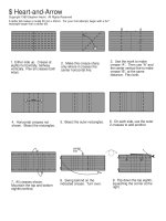
Figure 3: Given and , with , the formae are compatible only if .
The arrow shows the similarity set
.
Figure 4: The left-hand graph shows (schematically) the probability of selecting each point along the
axis under R
. The right-hand graph shows the corresponding diagram for standard crossover with
real genes.
Figure 5: The -dimensional R operator for real genes picks any point in the hypercuboid with
corners at the chromosomes being recombined,
and .
strips of arbitrary width. Thus, a forma might be a half-open interval with and
both lying in the range . These formae are separable. Respect requires that all children
are instances of any formae which contain both parents and . Clearly the similarity set of
and (the smallest interval which contains them both) is , where it has been assumed,
without loss of generality, that . Thus respect requires that all their children lie in .
Similarly, if is in some interval and lies in some other interval ,
then for these formae to be compatible the intersection of the intervals that define them must
be non-empty ( ; figure 3) and so picking a random element from the similarity set
allows any element that lies in the intersection to be picked, showing that R fulfils the
requirements of assortment (figure 4). The -dimensional R operator picks a random point
in the -dimensional hypercuboid with corners at the two chromosomes and (figure 5).
Both this operator and its natural analogue for -ary string representations, which for
each locus picks a random value in the range defined by the alleles from the two parents,
suffer from a bias away from the ends of the interval. It is therefore necessary to introduce a
mutation operator that offsets this bias in order to ensure that the whole search space remains
accessible. An appropriate mutation operator acts with very low probability to introduce the

extremal values at an arbitrary locus along the chromosome. In the one dimensional case
this amounts to occasionally replacing the value of one of the chromosomes with an or a
. The combination of R and such end-point mutation provides a surprisingly powerful set
of genetic operators for some problems, outperforming more common (binary) approaches
(Radcliffe, 1991a). The blend crossover operator BLX-0.5, which is a generalisation of R
developed by Eshelman & Schaffer (1992), performs even better.
Locality formae are not, of course, the only alternatives to schemata which can be applied
to real-valued problems, and there is no suggestion here that locality formae should be seen
as a generic or definitive alternative to schemata. It would be interesting, for example, to
attempt to construct formae and representations on the basis of fourier analysis, or some other
complete orthonormal set of functions over the space being searched.
Edge Formae for the Travelling Sales-rep Problem
The travelling sales-rep problem(TSP)isperhaps the most studiedcombinatorialoptimisation
problem, and has certainly attracted much effort with evolutionary algorithms. Given a set of
cities, the problem is to find the shortest route for a notional sales-rep to follow, visiting each
city exactly once. This problem has a number of important industrial applications, including
finding drilling paths for printed circuit boards to maximise production speed. It seems clear,
as Whitley et al. (1989b) have argued, that the edges rather than the vertices of the graph are
central to the TSP. While there might be some argument as to whether or not the edges should
be taken to be directed, the symmetry of the euclidean metric used in the evaluation function
suggests that undirected edges suffice.
If the towns (vertices) in an
-city TSP are numbered 1 to , and the edges are described
as non-ordered pairs of vertices
, then apparently suitable edge formae are simply sets
of edges, subject to the condition that every vertex appears in the description of exactly two
edges. These formae are not separable. To see this, consider two tours
and , with
containing the fragment 2–1–3 and containing 4–1–3. Plainly these have the common edge
(which is, of course, the same as ). Edge formae are described by the list of edges

they require to be present in angle brackets, so that
is an instance of the forma and
is an instance of the forma . These formae are clearly compatible, because any tour
containing the fragment 2–1–4 is in their intersection
Any recombination operator that respects these formae is bound to include the common edge
in all offspring from these parents. This precludes generating a child in .
Since assortment requires that this child be capable of being generated this shows that these
formae are not separable.
R can be defined for edge formae even though they are not separable: it works simply
by copying common edges into the child and then putting in random edges in such a way as
to complete a legal tour. The lack of separability simply ensures that R does not assort the
formae. Extensive experiments with R -related operators for the TSP are related in Radcliffe
& Surry (1994).
Curiously, the intersection operation for these edge formae looks like the set union operation. This is
because is really an abbreviation for the set of chromosomes containing the 1–3 edge.
Formae for Set Problems
A large number of optimisation problems are naturally formulated as subset extraction prob-
lems, i.e. given some “universal” set, find the best subset of it according to some criterion.
Examples include stock-marketportfoliooptimisation(Shapcott,1992), choosing
sites from
possible sites for retail dealers (George, 1994) and optimising the connectivity of a three
layer neural network (Radcliffe, 1993). If the size of the subset is not fixed, the natural way
to tackle this problem is by using a binary string the length of the universal set, using a 1
to indicate that the given element is in the subset. If, however, the size is fixed this is more
problematical, because this constrains the number of ones in the string. A more natural ap-
proach is to store the elements in the subset and apply appropriate genetic operators directly.
In this case the elements themselves can form alleles, and approaches as simple as choosing
the desired number of elements from those available between the parents can be effective.
This method happens to equate to use of RAR (Radcliffe, 1992b). Forma analysis for set
problems is covered extensively in Radcliffe (1992a).

General Representations
It has been argued in the preceding sections that there are theoretical, practical and empirical
motivations for moving away from the very simple binary string representations that have
dominated genetic algorithms for so long. Combined with the successes shown by genetic
programming, evolution strategies and evolutionary programming these form a compelling
case for supporting the use of arbitrary data structures as genetic representations. The way in
which RPL2 achieves this is discussed in section 5.
4 Parallelism
Evolutionary algorithms that use populations are inherently parallel in the sense that—
depending on the exact reproductive plan used—each chromosome update is to some extent
independent of the others. There are a number of options for implementation on parallel
computers, several of which have been proposed in the literature and implemented. As has
been emphasised, population structure has tended to be tied closely to the architecture of a
particular target machine to date, but there is no reason, in general, why this need be so.
Parallelism is supported in RPL2 at a variety of levels. Data decomposition of structured
populations can be achieved transparently, with different regions of the population evolving
on different processors, possibly partially synchronised by inter-process communication.
Distribution of fine-grained models tends to require more interprocess communication and
synchronisation so their efficiency is more sensitive to the computation-to-communications
ratio for the target platform.
Task farming of compute intensive tasks, such as genome evaluation (e.g. Verhoeven et
al., 1992; Starkweather et al., 1990), is also provided via the loop construct, which
indicates a set of operations to be performed on all members of a population stack in no fixed
order. This is particularly relevant to real-world optimisation tasks for which it is almost
invariably the case that the bulk of the time is spent on fitness evaluation. (For example see
section 6.) User operators may themselves include parallel code or run on parallel hardware
independently of the framework, giving yet more scope for parallelism.
RPL2willrunthesamereproductiveplanonserial, distributed or parallel hardware without
modification using the minimum degree of synchronisation consistent with the reproductive
plan specified.

5 System Architecture
RPL2 defines a C-like data-parallel language for describing reproductive plans. It is de-
signed to simplify drastically the task of implementing and experimenting with evolutionary
algorithms. Both parallel and serial implementations of the run-time system exist and will
execute the same plans without modification.
The language provides a small number of built-in constructs, along with facilities for
calling user-defined operators. Several libraries of such operators are provided with the
basic framework, as are definitions of several commonly used genetic representations. Two
example plans are presented at the end of this paper.
5.1 Language Features
RPL2 is a simple procedural language, similar to C, with six basic data types—
, ,
, , and . The genome and gstack types are explained further
below.
Simple control flow using
, , and are provided, as are normal algebraic
mathematical and logical expressions. User defined operators (C-callable functions) are
made visible as procedures in the language with the declaration, which is analogous to
C’s .
The data-parallel aspect of the language is supported using the concept of a population
structure, which is declared as a multi-dimensional hypercuboid. Arrays corresponding to
any combination of axes of the population structure may then be declared and manipulated
in a SIMD-like way (i.e. an operation on such an array affects every element within it).
Several special operators to project and reduce the dimensionality of such arrays are also
provided. Built-in constructs to support parallelism include two types of parallel loops—the
data-parallel , and a construct to indicate that data-independent farming
out of work is possible.
5.2 The RPL2 Framework
The RPL2 framework provides an implementation of the reproductive plan language based
on a interpreter and a run-time system, supported by various other modules. The diagram in

figure 6 shows how these different elements interact.
The interpreter acts in two main modes: interactive commands are processed immediately,
while non-interactive commands are compiled to an internal form as a reproductive plan
is being defined. Facilities also exist for batch processing, I/O redirection, and some on-
line help. The interpreted nature of the system is especially useful for fast turn-around
experimentation. The trade-off in speed over a compiled version is insignificant for real
applications in which almost all of the execution time is spent in the evaluation function. The
system uses the Marsaglia pseudo-random number generator (Marsaglia et al., 1990), which
as well as producing numbers with good statistical distributions allows identical results to be
produced on different processor architectures provided that they use the same floating point
representation.
Two versions of the run-time system exist, a serial (single-processor) implementation, and
a parallel (multiple distributed processors) implementation. In the serial case, both the parser
and the run-time system run on a single processor, and no communication is required. In
the parallel case, the parser runs on a single processor, but the work of actually executing
a reproductive plan is shared across other processors. Two methods for this work-sharing
are provided, one in which the data space of a structured population is decomposed across a
regular grid of processors and one in which extra processors are used simply as evaluation
servers for compute-intensive sections of code, typically evaluation of genome fitness. A
hybrid model in which the data space is distributed across some processors and others are
used as a pool of evaluation servers is planned as a future extension.
Parallelism by data-decomposition is made possible by the SIMD-like nature of the lan-
guage. In such a case, a structured population is typically declared and operations take
PNP2P0
Init
Parser
RTS
Serial Version
P0
Init

Parser
RTS
RD/TF
Comms
Init
RTS
RD/TF
Comms
Idle
Data, TF/RD
PLAN
endplan
endplan
endplan
P1
Parallel Version
. . .
"run" "run"
Figure 6: Simplified Execution Flow. The simplest mode of execution is the serial framework with
a single process, P0, in which actions are processed by the parser, and “compiled” code is executed by
the run time system. In parallel operation, the parser runs on a single process, and information about
the reproductive plan is shared by communication. A decision about how to execute the plan is made,
resulting either in the data space being split across the processes or in compute-intensive parts of the
code being task farmed.
place uniformly over various projections of the multi-dimensional space. Each processor can
then simply execute the common instructions over its local data, sharing information with
neighbouring processes when necessary.
Task farming is supported by the the
construct which allows the user to specify
a set of operations which apply to all genomes in population. This is illustrated in the first

example plan presented in the appendix.
Itwas stressed in sections 1and3earlierthatamajordesign aim forRPL2 was thatit should
impose no constraints on the data structures used to represent solutions. This is achieved by
providing a completely generic data structure which contains only information that
any type of genome would have. From the user’s point of view, this consists only of the
raw fitness value. A generic pointer is then included that references a user-definable data
structure, allowing a genome to be completely general. Collections of s are called
s, and admit the notionof scaled fitness, relative to other genomes in the group. These
data structures are illustrated in figure 7.
5.3 Extending the Framework
Ithasbecomeclearthatreal-worldapplicationsdemandgoodqualityproblem-specificgenome
representations, as discussed in section 3. The RPL2 system leaves the user completely free in
nElem
GSTACK
User Defined
User Defined
User Defined
. . .
NULL
GWRAP
scaledFitness
isScaled
GWRAP
scaledFitness
isScaled
GWRAP
scaledFitness
isScaled
GENOME
rawFitness

isEvaluated
GENOME
rawFitness
isEvaluated
GENOME
rawFitness
isEvaluated
Figure 7: Construction of a . A is made up of a linked list of structures,
each of which points at a
(allowing genomes be referenced in more thanone stack). A genome
has a scaled fitness only in the context of a stack, but has an absolute raw fitness. Each genome also
contains a pointer to the (user-defined) representation-dependent data.
his or her choice of representation: the framework works with generic genomes that include
a user-defined and user-manipulated component. This makes it equally suitable for all modes
of evolutionary computation from genetic algorithms and evolution strategies (Baeck et
al., 1991) to genetic programming (Koza, 1992), evolutionary programming (Fogel, 1993)
and hybrid schemes.
New operators and new genetic-representations are defined by writing standard ANSI
C-callable functions with return values and arguments corresponding to RPL2 data types.
A supplied preprocessor ( ) generates appropriate wrapper code to allow the operators
to be called dynamically at plan run-time (see the top of figure 8). Operator libraries may
optionally include initialisation and exit routines, start-up parameters, and check-pointing
facilities, supporting an extremely broad class of evolutionary computation. New represent-
ation libraries must also provide routines which allow the framework to pack, unpack and
free the user-defined component of a genome in order to permit representation-independent
cross-processor communication.
Adistinctionismadebetweenrepresentation-independentoperators,whose action depends
only on the standard fields of a genome (such as fitness measures), and representation-
dependent operators, which maymanipulate the problem-specific part. Examples of represen-
tation-independentoperatorsincludeselection mechanisms, replacement strategies, migration

and deme collection. All “genetic” operators (most commonly recombination, mutation and
inversion) are representation dependent, as are evaluation functions, local optimisers and
generators of random solutions.
This distinction strongly promotes code re-use as domain-independent operators can form
generic libraries. Even representation-dependent operators may have fairly wide applicability
since many different problems may share operators at the genetic level: it is only evaluation
functions that invariably have to be developed freshly for new problem domains.
Several libraries of operators and representations are provided with the framework, both
.h
Libname.h Makefile
libframework.a
Libname_rpp.c
.c
rpp
make
.c
rpl_lib_init.clibLibname.a
Makefile
rpl2
libRepname.alibRIOname.a
make
Building a library of operators
.h
Lib_hdr.h
.c
Lib_1.c
.c
Lib_2.c
libLibname.a
Building a customised version of RPL2

Figure 8: User Library Management. In the top half of the figure, is used to generate the
wrapper functions which interface between the RPL2 framework and the user’s C-callable code.
This code is compiled to generate a library of object code. Shown below is the process by which a
customised version of RPL2 is built. An interface function which calls the initialisationcode for each
library is generated from the list of libraries in the
. This is linked along with the requested
libraries and the framework code to produce the executable.
as examples for customisation, and to facilitate quick prototyping and development of applic-
ations. The supplied representations currently include real strings, binary strings, variable-
cardinality integer strings, sets, and permutations. A number of simple evaluation functions
are also included to allow initial familiarisation with the system before tackling a particular
application.
Customised versions of the framework are built by linking together whatever combination
of operator libraries and representations is desired, allowing locally developed operators to be
tested in the context of existing libraries, maintained in some central location. This is shown
in the bottom of figure 8.
Contributions of new libraries of operators and representations are solicited and will be
considered for inclusion with future general releases of RPL2, allowing even more scope for
code sharing and re-use.
6 Applications
6.1 Gas Network Pipe-Sizing
The problem of designing a gas supply network can be broken down into two essential
components—defining the routes that the pipes should follow and deciding the diameter of
each of the pipes. The choice of route is generally constrained to follow the road network
fairly closely and can be achieved efficiently by hand, but the process of selecting the pipe
sizes is more complex and requires optimisation.
Other things being equal, thinner pipes are preferable to thicker pipes because they are
cheaper, but the pipe network must also satisfy two implicit constraints. The first requires
that the network be capable of supplying all customer gas demands at or above a “minimum
design pressure”. The second, an engineering constraint, requires that every pipe in the

network should have at least one other pipe of equal or larger diameter “upstream” of it.
The problem is thus to determine the cheapest pipe network that can be constructed that
satisfies the two constraints. EPCC worked with British Gas on this problem, at the same
time as designing and implementing RPL2.
In the particular problem considered, the network contained 25 pipes, each of which could
be selected from six possible sizes, giving rise to a search space of size (about
thirty billion billion). The pipes connect 25 nodes, 23 of which are (varying) demand nodes
and two of which are pressure-defined source nodes (flow-defined source nodes may also be
specified). The network is a real one, that was actually installed (with pipe-sizes determined
using the existing heuristic method discussed below).
Genetic Representation
The representation used to represent the pipe sizes in the network is a variable cardinality
integer string. A genome is a sequence of
integers with ,
where is the cardinality (numberofalleles) of the th gene. The particular problem instance
tackled happened to have
for each pipe, but this is not generally the case.
This library is provided in RPL2 as
, and was supplemented for this work by a
sub-library of problem specific operators for evaluation and so forth.
Heuristic (Cost 17743.8)
Genetic Algorithm (Cost 17075.2)
Source
Demand
Pipe diameter
Figure 9: The genetic algorithm finds a solution approximately 4% cheaper (in cash terms) than that
found by the heuristic technique and actually used for the installed network. The networks are shown
only schematically: the pipes are actually of different lengths. The demand and supply requirements
are also different at each node. Both networks are valid in that they satisfy both the upstream-pipe
and minimum pressure constraints.

Evaluation Function
The evaluation function used determines the cost of a genome by summing the cost of the
pipes making up the network.
The satisfaction or non-satisfaction of the two constraints must however, also be con-
sidered. Both the upstream pipe constraint and the minimum pressure constraint are implicit.
Their satisfaction can only be determined by solving the non-linear gas flow equations in the
network which defines the upstream direction and the pressure at each node in the network.
A penalty function is really the only viable approach for handling implicit constraints such as
these, since it would be extremely difficult or impossible to construct genetic operators that
respected them. Ideas from Richardson et al. (1989), Michalewicz & Janikow (1991) and
Michalewicz (1993) were used to increase the penalty gradually as a function of generation
number.
The form of the cost function used was
(2)
where the first term is the cost of the pipes as a function of diameter, the second term is the
minimum pressure constraint, and the final term is the upstream pipe constraint. In this final
term, summation is over pipes where there is no upstream pipe which is of greater or equal
diameter and is the diameter of the largest upstream pipe from pipe .
Values were selected for the constants and that normalised nominal values of the
penalties to the same scale as the basic cost of the network. The exponents and were
selected in order to make the penalties grow at roughly the same rate as networks became
“worse” at satisfying the constraints. The annealing parameters and were subject to
experimentation.
The Reproductive Plan
A fairly conventional reproductive plan was developed to tackle the problem, using elitism
to preserve the best member of the population. Because the fitness of a genome depends
on penalty terms that vary with the current generation number, the entire population must
be re-evaluated at each generation, prior to fitness-based reproduction. Various forms of
structured populations were investigated during the problem, using the facilities provided by
RPL2. A panmictic (unstructured) population was used in most initial experiments, in order

to tune values of parameters, particularly for the fitness function. A fine-grained structure did
not yield significant benefits, perhaps due to the relative simplicity of the problem. An island
structure was also used, with the main benefit being the ability to run on multiple processors
and try longer runs with larger populations. However, this also did not significantly improve
performance.
Results
The heuristic technique in previous operationaluse by British Gas was applied to theproblem,
in order to compare its performance to the genetic approach. The installed network was
actually designed using the results obtained from the heuristic.
The heuristic determines a good configuration of pipe sizes by first assuming a constant
pressure drop over the whole network and guessing some initial pipe sizes that will yield a
valid but not necessarily optimal network. The heuristic proceeds by locally optimising this
solution, repeatedly trying to reduce single pipe diameters while maintaining a valid network.
Eventually this process terminates when no pipe size can be reduced while maintaining
network validity. The algorithm takes on the order of ten seconds on a 486 PC (25MHz)
to reach its “optimal” configuration for the problem under study. A schematic (which does
not represent differences in pipe lengths and source/demand requirements) of this solution
appears in the left-hand part of figure 9.
The genetic technique produced consistently good results, although it did not always
converge to the same optimal solution. In most cases it found networks which were better,
often significantly so, than that determined by the heuristic approach. In almost all cases
the algorithm found a valid network by the end of the run (i.e. one in which the penalty
terms were zero). Run times for typical populations of 100 networks through 100 generations
(testing at most 10,000 different networks) were of the order of several minutes on a Sun
SPARC 2 workstation. Note however that the increased cost of this computer time over that
of the heuristic is trivial relative to the savings in pipeline construction. The best result was a
network approximately 4% cheaper than the heuristic solution. A schematic of this network
is shown in the right-hand part of figure 9.
This project has clearly demonstrated to British Gas that genetic algorithms and RPL2
can produce cost savings on real business problems. British Gas now intends to adopt this

powerful solution technique for a number of other problems.
6.2 Retail Dealership Location
Geographical Modelling and Planning (GMAP) Ltd. specialises in the planning of efficient
delivery networks for goods and services. In particular, GMAP helps its clients to optimise
their networks of dealerships or retail outlets. In order to achieve this goal, a mathematical
model has been developed that predicts the pattern and volume of business expected from
a given distribution network by integrating demographic, geographic and marketing inform-
ation. The model used—a so-called spatial interaction model—provides a highly complex
function to be optimised. GMAP’s approach had been to use a heuristic to search for deal-
ership networks with high levels of predicted sales within single regions of Britain, of which
there are sixteen.
Working collaboratively with GMAP, Felicity George (1994) first produced a parallel
implementation of the spatial interaction model and heuristic on a Connection Machine
CM-200. This ran some 2,500 times faster than the sequential implementation on a Sun
SPARCstation. This reduced the (projected) run-timefor the heuristic on the whole of Britain
from a matter of a few months to around an hour, and facilitated the tackling of this problem
with genetic search techniques.
The prototype implementation of RPL2—RPL Russo (1991)—was used to construct a
hybrid genetic algorithm for this problem. RPL ran on the front end of the Connection
Machine while the evaluation function (the spatial interaction model) and the heuristic ran
on the Connection Machine itself. The problem of choosing the optimal dealer network is
naturally formulated as a subset extraction problem (choosing in which of Britain’s 8,500
postal districts dealerships should exist) so the forma analysis of set problems reviewed in
section 3.5 was exploited. R
provided good results, as did a spatial recombination operator
designed especially for the problem. The spatial operator exchanges geographical clusters
between parents while using directed mutations around boundaries to keep the number of
dealers fixed. The results were improved still further, as expected, when the pure genetic
algorithm was augmented by incorporating a pseudo-genetic operator based on the original
heuristic used by GMAP.

Network Solutions
The three diagrams below show small dealer networks found by the original heuristic tech-
nique, by a pure genetic algorithm and by a hybrid genetic algorithm. In this case, the hybrid
genetic algorithm produces results some 6% better than those found by the heuristic. Larger
networks can also be designed, allowing larger scope for improvements over the heuristic
technique, but are harder to visualise. The investigations carried out covered a wide range of
network sizes and in all cases providedresulting networks with predictedsales levels between
5% and 20% higher than those found by the heuristic.
Original heuristic
(sales 19107)
Pure GA
(sales 20187)
Hybrid GA
(sales 20264)
The hybrid genetic algorithm implementation has further advantages over the heuristic. It
allows the existing network to be taken as a starting point and perturbed to produce a better
network, thus allowing incremental improvement to the network as well as the design of
complete networks from scratch. Moreover, genetic search allows the construction of a range
of high-quality solutions thus permitting the decision maker to choose from a number of good
networks. This allows additional decision criteria to be incorporated, including those that
may not be straightforward to compute, such as more subjective considerations.
6.3 Data Mining
Large organisations routinely gather vast and ever-increasing amounts of data in the ordinary
course of their business. While the information is typically collected with a specific purpose
in mind, once collated it also has the potential to be exploited for other purposes. There is
increasing interest in the production of systems for performingautomatic inductive reasoning
conditioned by the data residing in such databases, in the process becoming known as data
mining (Holsheimer & Siebes, 1994).
As a general concept, data mining is intuitively appealing but rather poorly defined. Many
different formulations can be imagined, and each will lead to different detailed goals, forms

for the discovered knowledge and—presumably—rates of success.
Data mining has as its goal the discovery and elucidation of interesting and useful patterns
withina database. Theemphasis ison novel patterns, whichin this context means patterns that
humans find hard to extract either by eye or using standard look-up or statistical techniques.
The most useful form in which the results of data mining can be presented is as explicit rules,
perhaps expressed as predicates (if then ). It is not necessary for rules to be strictly correct
in order for them to be useful, and indeed in general this is a stronger requirement than one
would wish to impose. Picking out trends and correlations that are true to some degree is
the more typical aim, because data is generally noisy in the true sense of containing errors,
and more importantly because correlations do not have to hold perfectly in order to constitute
useful, exploitable information.
While data mining in its purest form is thought of as a (relatively) undirected search, in
that the subject of the rules to be found is not normally specified, expressing knowledge in
the form of rules makes it straightforward to restrict some part of the rule and thus to direct
the data miner towards particular kinds of knowledge discovery.
While the discovery of rules is in an intuitive sense a “search” problem, there is much
freedom in its casting as a well-defined search or optimisation task. It is clear that the goal
is not simply to find the single “best” rule describing the database, not only because “best” is
extremely difficult to quantitatively define, but because the goal is to find a selection of rules
representing different kinds and instances of patterns within the database. Thus the problem
has a covering aspect to it. Presumably rules will form clusters and it seems natural to try to
collect one (good) representativefrom each cluster of similar rules surpassing some minimum
quality.
In the context of evolutionary computing this raises a host of interesting possible ap-
proaches. While traditional genetic algorithms and evolution strategies have most often been
applied to strict optimisation problems, there are numerous techniques for encouraging nich-
ing and speciation. Current work on data mining at EPCC uses structured population models
to encourage niching. The covering ability of the resultant genetic algorithm is then further
enhanced by exploiting a two-level hierarchical scheme, described below.
The Hierarchical Genetic Algorithm

It has been emphasised already that the goal of data mining is to discover not a single rule
but a useful collection of different rules. To achieve this, genetic algorithms operating at
two different levels of a hierarchy are used. The “low-level” genetic algorithms searches
for individual rules competitively, using a fine-grained structured population to encourage a
degree of speciation. A higher level genetic algorithm then takes rules generated by the lower
level algorithms and uses them as basic “genetic material” from which to form sets of rules
using techniques for genetic set-based optimisation discussed in section 3.5.
More precisely, rules are taken from each of the low-level populations to form a universal
set of rules from which it will be the task of the high-level genetic algorithm to find the “best”
set of some given size—for example, the best set of twenty rules. Notice that this is not to say
that the high-level genetic algorithm seeks to find(say) the twenty best rules: in thehigh-level
genetic algorithm the fitness function is applied to entire sets of rules and it is these sets that
compete. The aim is to find the best collection of rules with regard to a balance of rules with
different characteristics. In this manner, competition at two different levels of the hierarchy
results in the discovery of co-operatively useful sets of rules. This is shown schematically in
figure 10, and is of general relevance to covering problems: the low-level populations search
for good areas of the search space and the high-level population combines these into useful
coverages.
a
b
c
d
e
f
gi
j
k
l
m
n

o
p
r
s
t
w
x
y
z
u
q
v
h
m
t
q
c
vh
p
x
f
c
l
e
s
b
gq
u
. . . .
d

s
z
n
d
g
l
o
Low−level fine−grained
populations
Best rules found
at low−level form
{ g o l d }
{ z o n d }
{ g o l d }
{ z g d l }
{ s d g n }
universal set of rules
for high−level algorithm
High−level population
of rule sets
Search space of all possible rules
found at high−level
Best set of rules
Figure 10: The hierarchical genetic algorithm. The low-level genetic algorithms use structured
populations to search competitively for individual rules (or more generally, good candidate elements
for a set). The high-level genetic algorithm searches for the best set of rules it can form using those
individual rules generated by the low-level genetic algorithms (or, in general, the best set it can form
from the elements found by the low-level genetic algorithms).
A suitable evaluation function for the high-level algorithm is arrived at by considering the
characteristics sought from collections of rules discovered by the data miner. Clearly each

rule should be of high utility, but perhaps more importantly the rules presented ought to be
significantly different from one another, covering as many different rule types as possible. In
the present implementation coverage has been chosen as the key criterion, but in the longer
term the search will be cast as a multi-criterion problem at the higher level.
The Low-Level Genetic Algorithm
The low-level genetic search is used to find a number of interesting characterisations (rules)
of the database, to be used in the high-level algorithm to cover the space of interesting rules.
The data used in this work is week-on-week sales data from a major high-street grocery
retailer. The database holds information for 156 products over 55 weeks. Data is divided into
12 fields such as price, quantity sold, supplier and promotional information. The database is
augmented by weather information corresponding tothe sales periods, withfigures for weekly
average precipitation, minimum and maximum temperature and hours of sun. Each field in
the database can be viewed as a function of product and time, as it has a unique value for
each such pair. Weather data of course only varies as a function of time, being constant with
respect to product.
Fields are distinguished as either dependent or independent. Independent fields are values
that are not thought to be functions of other fields in the database, or are otherwise outside
the scope of the database. Dependent fields are those which might in principle be functions
of other data in the database, and about which the data-miner attempts to theorise. In
experiments conducted to date, quantity sold and total value of product sold are the only
dependent categories.
Rules
In this work, a rule is an if then predicate made up of three parts—the specificity (
), a number
of conditional clauses ( ), and a predictive clause ( ). Thus a rule is of form:
if and and and and then (3)
The specificity indicates which part of the domain of the database the rule applies to (in
terms of products and times). It currently specifies a contiguous range of time values and
either a single product or “all products” (e.g. bananas ).
The conditional part of the rule is formed by the conjunction (logical and) of a number

of simple clauses. Each clause is a linear inequality between one or two fields in the
database. For enumerated fields, the clause simply fixes some field (e.g. promotional position
:= “BIN6”). For two continuous fields, the clause relates their normalised values in an
inequality with two arbitrary real constants. The second field in the clause may contain a
time lag, and may be with respect to a different product. This allows the data-miner, for
instance, to relate the price of apples today to the number of oranges sold two weeks ago (e.g.
price apples today price oranges last week ).
The prediction part of the rule is a single clause. This clause is identical in form to those in
the conditional part of the rule except that one of the fields in the clause must be a dependent
category from the database. This excludes rules that theorise about relationships among
purely independent variables, which may or may not be true, but are certainly not relevant.
The fitness ofa rule is determinedbyhow well it appliesto the database, but this evaluation
function will not be discussed in detail here.
The Reproductive Plan
Within the hierarchical genetic algorithm, the low-level search produces a number of good
quality rules that form the basis for a coverage of the space of all interesting rules. Thus it is
not desirable for the search to converge to the same rule in each low-level population: rather
the aim is to cover many local optima.
The reproductive plan uses a fine-grainedpopulation structure in order to promote niching
in the search for rules. This assists the finding of many good rules. A number of low-level
searches are performed, and the results are collected for use as the universal set for the high-
level genetic algorithm (see figure 10). In the future, feedback from the high-level search
will direct the low-level genetic algorithms to search new regions, or to avoid highly covered
areas.
At each step, a child is formed by crossing the current genome with a member of its
deme (neighbourhood) chosen by binary-tournament selection (with replacement). The child
is mutated and evaluated, and possibly replaces the current parent using binary-tournament
replacement. After a specified number of generations, the best rule is saved for use in the
high-level algorithm, and the process is repeated.
A simple reproductive plan was also written for the high-level search. In current experi-

ments a panmictic (unstructured) population is used to search a universal set of 200 rules for
good subsets of size five.
During each generation, the population is incrementally replaced. A child is formed by
crossing two parentschosen usingbinary-tournamentselection. The resulting child is mutated
and evaluated, and added back into the population using binary-tournament replacement.
After a specified number of generations, the best collection is presented to the user.
Statistical measures such as population variance could also be used as stopping criteria.
Results
Results from the technique are still preliminary, as the work is in progress. However, both
the low-level and high-level algorithms appear to be functioning correctly and producing at
least some interesting results. Some examples rules produced by the low-level search are:
For golden delicious apples during the final 44 weeks of data, if the average sunshine (in
hours) plus 5.4 times the retail price (in pounds) is greater than 9.5 then the total value
of of apples sold is greater than £632.
For oranges during the first 50 weeks of data, if the average maximum temperature is
greater than
and the average rainfall is greater than 0.4 mm then the total value (in
pounds) plus 0.7 times the quantity sold five weeks ago will be greater than 423.
For bananas, if the average rainfall is less than 1.5mm then more than 1373 lbsofbananas
will be sold.
The higher-level algorithm does tend to produce collections of dissimilar rules with high
fitness, as expected. However, further investigation and analysis of the results are required
before more detailed conclusions can be drawn.
6.4 Other Applications
A number of other applications have been tackled using RPL2 and its predecessor, RPL.
These include the Travelling Sales-rep Problem using a permutation representation with
Random Assorting Recombination (Radcliffe, 1994a), stock market tracking with a hybrid
scheme based on a set-based representation (Shapcott, 1992) and neural network topology
optimisation (Dewdney, 1992). Trivial test problems using binary representations have also
been implemented for demonstration purposes.

Availability
The RPL2 framework, along with a variety of common representation libraries, is distributed
without charge. The language interpreter and run-time system is provided in object form
while source code is provided for the representation libraries, to allow users to study and
modify them. The distribution includes high quality manuals, providing not only reference
material for RPL2 but general genetic algorithm reference and a tutorial modelled on that of
Davis (1991).
Portability across architectures is an important feature of RPL2, allowing exactly the same
reproductive plans to be run on a wide variety of platforms. This has been achieved by
basing the software on portable tools, both for compilation and inter-process communication.
A serial version of the system requires only the widely available compiler generation tools
and , and an ANSI-C compiler. EPCC’s CHIMP communications interface, and a
number of parallel utility library modules have been used in the parallel version.
The CHIMP communications software is currently available on the following systems:
Sun SPARCstation, Silicon Graphics Workstation, IBM RS/6000 Workstation, DEC Alpha
Workstation, Sequent Symmetry, Meiko Computing Surface 1, Meiko Concerto, and the
Meiko Computing Surface 2. It is planned that RPL2 will migrate to the emerging MPI
standard for message-passing, to ensure an even wider range of host hardware, including
such platforms as: Cray T3D, Fujitsu AP1000, Intel iPSC, Intel Paragon, Thinking Machines
CM5, and the IBM SP1.
Inquiries concerning RPL2 are welcomed by email to
.
Acknowledgements
The serial prototype of RPL2 was implemented by Claudio Russo (1991), who developed many of
the ideas with Nicholas Radcliffe. The parallel prototype was developed by Graham Jones (1992).
Mark Green and Ian Boyd from British Gas worked together with Patrick Surry on the design and
implementation of RPL2. The work on retail dealership location with Ford was undertaken primarily
by Felicity George (EPCC) in collaboration with GMAP Ltd.
Appendix: Example RPL2 plans
Panmictic example

1
2
3
4
5
6
7
8
9
10
11
12
13
14
15
16
17
18
19
20
21
22
23
24
25
26
27
28
29
30

31
32
33
34
35
36
37
38
39
40
41
42
43
44
45
46
47
48
49
50
51
52
53
54
55
56