Tài liệu Đề tài " On the volume of the intersection of two Wiener sausages " ppt
Bạn đang xem bản rút gọn của tài liệu. Xem và tải ngay bản đầy đủ của tài liệu tại đây (906.14 KB, 44 trang )
Annals of Mathematics
On the volume of the
intersection of two
Wiener sausages
By M. van den Berg, E. Bolthausen, and F. den
Hollander
Annals of Mathematics, 159 (2004), 741–783
On the volume of the intersection
of two Wiener sausages
By M. van den Berg, E. Bolthausen, and F. den Hollander
Abstract
For a>0, let W
a
1
(t) and W
a
2
(t)bethea-neighbourhoods of two indepen-
dent standard Brownian motions in R
d
starting at 0 and observed until time
t. We prove that, for d ≥ 3 and c>0,
lim
t→∞
1
t
(d−2)/d
log P
|W
a
1
(ct) ∩ W
a
2
(ct)|≥t
= −I
κ
a
d
(c)
and derive a variational representation for the rate constant I
κ
a
d
(c). Here, κ
a
is the Newtonian capacity of the ball with radius a. We show that the optimal
strategy to realise the above large deviation is for W
a
1
(ct) and W
a
2
(ct) to “form
a Swiss cheese”: the two Wiener sausages cover part of the space, leaving
random holes whose sizes are of order 1 and whose density varies on scale t
1/d
according to a certain optimal profile.
We study in detail the function c → I
κ
a
d
(c). It turns out that I
κ
a
d
(c)=
Θ
d
(κ
a
c)/κ
a
, where Θ
d
has the following properties: (1) For d ≥ 3: Θ
d
(u) < ∞
if and only if u ∈ (u
, ∞), with u
a universal constant; (2) For d =3: Θ
d
is
strictly decreasing on (u
, ∞) with a zero limit; (3) For d =4: Θ
d
is strictly
decreasing on (u
, ∞) with a nonzero limit; (4) For d ≥ 5: Θ
d
is strictly
decreasing on (u
,u
d
) and a nonzero constant on [u
d
, ∞), with u
d
a constant
depending on d that comes from a variational problem exhibiting “leakage”.
This leakage is interpreted as saying that the two Wiener sausages form their
intersection until time c
∗
t, with c
∗
= u
d
/κ
a
, and then wander off to infinity in
different directions. Thus, c
∗
plays the role of a critical time horizon in d ≥ 5.
We also derive the analogous result for d = 2, namely,
lim
t→∞
1
log t
log P
|W
a
1
(ct) ∩ W
a
2
(ct)|≥t/ log t
= −I
2π
2
(c),
∗
Key words and phrases. Wiener sausages, intersection volume, large deviations, vari-
ational problems, Sobolev inequalities.
742 M. VAN DEN BERG, E. BOLTHAUSEN, AND F. DEN HOLLANDER
where the rate constant has the same variational representation as in d ≥ 3
after κ
a
is replaced by 2π. In this case I
2π
2
(c)=Θ
2
(2πc)/2π with Θ
2
(u) < ∞
if and only if u ∈ (u
, ∞) and Θ
2
is strictly decreasing on (u
, ∞) with a zero
limit.
Acknowledgment. Part of this research was supported by the Volkswagen-
Stiftung through the RiP-program at the Mathematisches Forschungsinstitut
Oberwolfach, Germany. MvdB was supported by the London Mathematical
Society. EB was supported by the Swiss National Science Foundation, Contract
No. 20-63798.00.
1. Introduction and main results: Theorems 1–6
1.1. Motivation. In a paper that appeared in “The 1994 Dynkin
Festschrift”, Khanin, Mazel, Shlosman and Sinai [9] considered the following
problem. Let S(n),n∈ N
0
, be the simple random walk on Z
d
and let
R = {z ∈ Z
d
: S(n)=z for some n ∈ N
0
}(1.1)
be its infinite-time range. Let R
1
and R
2
be two independent copies of R and
let P denote their joint probability law. It is well known (see Erd¨os and Taylor
[7]) that
P (|R
1
∩ R
2
| < ∞)=
0if1≤ d ≤ 4,
1ifd ≥ 5.
(1.2)
What is the tail of the distribution of |R
1
∩R
2
| in the high-dimensional case?
In [9] it is shown that for every d ≥ 5 and δ>0 there exists a t
0
= t
0
(d, δ)
such that
exp
− t
d−2
d
+δ
≤ P
|R
1
∩ R
2
|≥t
≤ exp
− t
d−2
d
−δ
∀t ≥ t
0
.(1.3)
Noteworthy about this result is the subexponential decay. The following prob-
lems remained open:
(1) Close the δ-gap and compute the rate constant.
(2) Identify the “optimal strategy” behind the large deviation.
(3) Explain where the exponent (d−2)/d comes from (which seems to suggest
that d = 2, rather than d = 4, is a critical dimension).
In the present paper we solve these problems for the continuous space-time
setting in which the simple random walks are replaced by Brownian motions
and the ranges by Wiener sausages, but only after restricting the time horizon
to a multiple of t. Under this restriction we are able to fully describe the
large deviations for d ≥ 2. The large deviations beyond this time horizon will
ON THE VOLUME OF THE INTERSECTION OF TWO WIENER SAUSAGES
743
remain open, although we will formulate a conjecture for d ≥ 5 (which we plan
to address elsewhere).
Our results will draw heavily on some ideas and techniques that were
developed in van den Berg, Bolthausen and den Hollander [3] to handle the
large deviations for the volume of a single Wiener sausage. The present paper
can be read independently.
Self-intersections of random walks and Brownian motions have been stud-
ied intensively over the past fifteen years (Lawler [10]). They play a key role
e.g. in the description of polymer chains (Madras and Slade [13]) and in renor-
malisation group methods for quantum field theory (Fern´andez, Fr¨ohlich and
Sokal [8]).
1.2. Wiener sausages. Let β(t), t ≥ 0, be the standard Brownian motion
in R
d
– the Markov process with generator ∆/2 – starting at 0. The Wiener
sausage with radius a>0 is the random process defined by
W
a
(t)=
0≤s≤t
B
a
(β(s)),t≥ 0,(1.4)
where B
a
(x) is the open ball with radius a around x ∈ R
d
.
Let W
a
1
(t), t ≥ 0, and W
a
2
(t), t ≥ 0, be two independent copies of (1.4),
let P denote their joint probability law, let
V
a
(t)=W
a
1
(t) ∩ W
a
2
(t),t≥ 0,(1.5)
be their intersection up to time t, and let
V
a
= lim
t→∞
V
a
(t)(1.6)
be their infinite-time intersection. It is well known (see e.g. Le Gall [11]) that
P (|V
a
| < ∞)=
0if1≤ d ≤ 4,
1ifd ≥ 5,
(1.7)
in complete analogy with (1.2). The aim of the present paper is to study the
tail of the distribution of |V
a
(ct)| for c>0 arbitrary. This is done in Sections
1.3 and 1.4 and applies for d ≥ 2. We describe in detail the large deviation
behaviour of |V
a
(ct)|, including a precise analysis of the rate constant as a
function of c. In Section 1.5 we formulate a conjecture about the large deviation
behaviour of |V
a
| for d ≥ 5. In Section 1.6 we briefly look at the intersection
volume of three or more Wiener sausages. In Section 1.7 we discuss the discrete
space-time setting considered in [9]. In Section 1.8 we give the outline of the
rest of the paper.
1.3. Large deviations for finite-time intersection volume.Ford ≥ 3, let
κ
a
= a
d−2
2π
d/2
/Γ(
d−2
2
) denote the Newtonian capacity of B
a
(0) associated
with the Green’s function of (−∆/2)
−1
. Our main results for the intersection
volume of two Wiener sausages over a finite time horizon read as follows:
744 M. VAN DEN BERG, E. BOLTHAUSEN, AND F. DEN HOLLANDER
Theorem 1. Let d ≥ 3 and a>0. Then, for every c>0,
lim
t→∞
1
t
(d−2)/d
log P
|V
a
(ct)|≥t
= −I
κ
a
d
(c),(1.8)
where
I
κ
a
d
(c)=c inf
φ∈Φ
κ
a
d
(c)
R
d
|∇φ|
2
(x)dx
(1.9)
with
Φ
κ
a
d
(c)=
φ ∈ H
1
(R
d
):
R
d
φ
2
(x)dx =1,
R
d
1 − e
−κ
a
cφ
2
(x)
2
dx ≥ 1
.
(1.10)
Theorem 2. Let d =2and a>0. Then, for every c>0,
lim
t→∞
1
log t
log P
|V
a
(ct)|≥t/ log t
= −I
2π
2
(c),(1.11)
where I
2π
2
(c) is given by (1.9) and (1.10) with (d, κ
a
) replaced by (2, 2π).
Note that we are picking a time horizon of length ct and are letting t →∞
for fixed c>0. The sizes of the large deviation, t respectively t/ log t, come
from the expected volume of a single Wiener sausage as t →∞, namely,
E|W
a
(t)|∼
κ
a
t if d ≥ 3,
2πt/ log t if d =2,
(1.12)
as shown in Spitzer [14]. So the two Wiener sausages in Theorems 1 and 2 are
doing a large deviation on the scale of their mean.
The idea behind Theorem 1 is that the optimal strategy for the two Brow-
nian motions to realise the large deviation event {|V
a
(ct)|≥t} is to behave
like Brownian motions in a drift field xt
1/d
→ (∇φ/φ)(x) for some smooth
φ: R
d
→ [0, ∞) during the given time window [0,ct]. Conditioned on adopting
this drift:
– Each Brownian motion spends time cφ
2
(x) per unit volume in the neigh-
bourhood of xt
1/d
, thus using up a total time t
R
d
cφ
2
(x)dx. This time
must equal ct, hence the first constraint in (1.10).
– Each corresponding Wiener sausage covers a fraction 1 − e
−κ
a
cφ
2
(x)
of
the space in the neighbourhood of xt
1/d
, thus making a total intersection
volume t
R
d
(1 − e
−κ
a
cφ
2
(x)
)
2
dx. This volume must exceed t, hence the
second constraint in (1.10).
The cost for adopting the drift during time ct is t
(d−2)/d
R
d
c|∇φ|
2
(x)dx. The
best choice of the drift field is therefore given by minimisers of the variational
problem in (1.9) and (1.10), or by minimising sequences.
ON THE VOLUME OF THE INTERSECTION OF TWO WIENER SAUSAGES
745
Note that the optimal strategy for the two Wiener sausages is to “form a
Swiss cheese”: they cover only part of the space, leaving random holes whose
sizes are of order 1 and whose density varies on space scale t
1/d
(see [3]). The
local structure of this Swiss cheese depends on a. Also note that the two
Wiener sausages follow the optimal strategy independently. Apparently, under
the joint optimal strategy the two Brownian motions are independent on space
scales smaller than t
1/d
.
1
A similar optimal strategy applies for Theorem 2, except that the space
scale is
t/ log t. This is only slightly below the diffusive scale, which explains
why the large deviation event has a polynomial rather than an exponential cost.
Clearly, the case d =2iscritical for a finite time horizon. Incidentally, note
that I
2π
2
(c) does not depend on a. This can be traced back to the recurrence
of Brownian motion in d = 2. Apparently, the Swiss cheese has random holes
that grow with time, washing out the dependence on a (see [3]).
There is no result analogous to Theorems 1 and 2 for d = 1: the variational
problem in (1.9) and (1.10) certainly continues to make sense for d = 1, but it
does not describe the Wiener sausages: holes are impossible in d =1.
1.4. Analysis of the variational problem. We proceed with a closer
analysis of (1.9) and (1.10). First we scale out the dependence on a and c.
Recall from Theorem 2 that κ
a
=2π for d =2.
Theorem 3. Let d ≥ 2 and a>0.
(i) For every c>0,
I
κ
a
d
(c)=
1
κ
a
Θ
d
(κ
a
c),(1.13)
where Θ
d
:(0, ∞) → [0, ∞] is given by
Θ
d
(u) = inf
∇ψ
2
2
: ψ ∈ H
1
(R
d
), ψ
2
2
= u,
(1 − e
−ψ
2
)
2
≥ 1
.(1.14)
(ii) Define u
= min
ζ>0
ζ(1 − e
−ζ
)
−2
=2.45541 Then Θ
d
= ∞ on
(0,u
] and 0 < Θ
d
< ∞ on (u
, ∞).
(iii) Θ
d
is nonincreasing on (u
, ∞).
(iv) Θ
d
is continuous on (u
, ∞).
(v) Θ
d
(u) (u −u
)
−1
as u ↓ u
.
Next we exhibit the main quantitative properties of Θ
d
.
1
To prove that the Brownian motions conditioned on the large deviation event {|V
a
(ct)|
≥ t} actually follow the “Swiss cheese strategy” requires substantial extra work. We will not
address this issue here.
746 M. VAN DEN BERG, E. BOLTHAUSEN, AND F. DEN HOLLANDER
Theorem 4. Let 2 ≤ d ≤ 4. Then u → u
(4−d)/d
Θ
d
(u) is strictly decreas-
ing on (u
, ∞) and
lim
u→∞
u
(4−d)/d
Θ
d
(u)=µ
d
,(1.15)
where
µ
d
=
inf
∇ψ
2
2
: ψ ∈ H
1
(R
d
), ψ
2
=1, ψ
4
=1
if d =2, 3,
inf
∇ψ
2
2
: ψ ∈ D
1
(R
4
), ψ
4
=1
if d =4,
(1.16)
satisfying 0 <µ
d
< ∞.
2
Theorem 5. Let d ≥ 5 and define
η
d
= inf{∇ψ
2
2
: ψ ∈ D
1
(R
d
),
(1 − e
−ψ
2
)
2
=1}.(1.17)
(i) There exists a radially symmetric, nonincreasing, strictly positive min-
imiser ψ
d
of the variational problem in (1.17), which is unique up to transla-
tions. Moreover, ψ
d
2
2
< ∞.
(ii) Define u
d
= ψ
d
2
2
. Then u → θ
d
(u) is strictly decreasing on (u
,u
d
)
and
Θ
d
(u)=η
d
on [u
d
, ∞).(1.18)
0
s
u
u
d
η
d
(iii)
0 u
µ
4
(ii)
0 u
(i)
Figure 1 Qualitative picture of Θ
d
for: (i) d =2, 3; (ii) d = 4; (iii) d ≥ 5.
Theorem 6. (i) Let 2 ≤ d ≤ 4 and u ∈ (u
, ∞) or d ≥ 5 and u ∈ (u
,u
d
].
Then the variational problem in (1.14) has a minimiser that is strictly positive,
radially symmetric (modulo translations) and strictly decreasing in the radial
component. Any other minimiser is of the same type.
(ii) Let d ≥ 5 and u ∈ (u
d
, ∞). Then the variational problem in (1.14)
does not have a minimiser.
2
We will see in Section 5 that µ
4
= S
4
, the Sobolev constant in (4.3) and (4.4).
ON THE VOLUME OF THE INTERSECTION OF TWO WIENER SAUSAGES
747
We expect that in case (i) the minimiser is unique (modulo translations).
In case (ii) the critical point u
d
is associated with “leakage” in (1.14); namely,
L
2
-mass u − u
d
leaks away to infinity.
1.5. Large deviations for infinite-time intersection volume. Intuitively,
by letting c →∞in (1.8) we might expect to be able to get the rate constant
for an infinite time horizon. However, it is not at all obvious that the limits
t →∞and c →∞can be interchanged. Indeed, the intersection volume might
prefer to exceed the value t on a time scale of order larger than t, which is not
seen by Theorems 1 and 2. The large deviations on this larger time scale are
a whole new issue, which we will not address in the present paper.
Nevertheless, Figure 1(iii) clearly suggests that for d ≥ 5 the limits can
be interchanged:
Conjecture. Let d ≥ 5 and a>0. Then
lim
t→∞
1
t
(d−2)/d
log P
|V
a
|≥t
= −I
κ
a
d
,(1.19)
where
I
κ
a
d
= inf
c>0
I
κ
a
d
(c)=I
κ
a
d
(c
∗
)=
η
d
κ
a
(1.20)
with c
∗
= u
d
/κ
a
.
The idea behind this conjecture is that the optimal strategy for the two
Wiener sausages is time-inhomogeneous: they follow the Swiss cheese strategy
until time c
∗
t and then wander off to infinity in different directions. The
critical time horizon c
∗
comes from (1.13) and (1.18) as the value above which
c → I
κ
a
d
(c) is constant (see Fig. 1(iii)). During the time window [0,c
∗
t] the
Wiener sausages make a Swiss cheese parametrised by the ψ
d
in Theorem
5; namely, (1.9) and (1.10) have a minimising sequence (φ
j
) converging to
φ =(c
∗
κ
a
)
−1/2
ψ
d
in L
2
(R
d
).
We see from Figure 1(ii) that d =4iscritical for an infinite time horizon.
In this case the limits t →∞and c →∞apparently cannot be interchanged.
Theorem 4 shows that for 2 ≤ d ≤ 4 the time horizon in the optimal
strategy is c = ∞, because c → I
κ
a
d
(c) is strictly decreasing as soon as it
is finite (see Fig. 1(i–ii)). Apparently, even though lim
t→∞
|V
a
(t)| = ∞ P -
almost surely (recall (1.7)), the rate of divergence is so small that a time of
order larger than t is needed for the intersection volume to exceed the value
t with a probability exp[−o(t
(d−2)/d
)] respectively exp[−o(log t)]. So an even
larger time is needed to exceed the value t with a probability of order 1.
1.6. Three or more Wiener sausages. Consider k ≥ 3 independent
Wiener sausages, let V
a
k
(t) denote their intersection up to time t, and let
748 M. VAN DEN BERG, E. BOLTHAUSEN, AND F. DEN HOLLANDER
V
a
k
= lim
t→∞
V
a
k
(t). Then the analogue of (1.7) reads (see e.g. Le Gall [11])
P (|V
a
k
| < ∞)=
0if1≤ d ≤
2k
k−1
,
1ifd>
2k
k−1
.
(1.21)
The critical dimension 2k/(k −1) comes from the following calculation:
E|V
a
k
| =
R
d
P
σ
B
a
(x)
< ∞
k
dx =
R
d
1 ∧
a
|x|
d−2
k
dx,(1.22)
where σ
B
a
(x)
= inf{t ≥ 0: β(t) ∈ B
a
(x)}. The integral converges if and only
if (d − 2)k>d.
It is possible to extend the analysis in Sections 1.3 and 1.4 in a straight-
forward manner, leading to the following modifications (not proved in this
paper):
(1) Theorems 1 and 2 carry over with:
– V
a
replaced by V
a
k
;
– c replaced by kc/2 in (1.9);
–
R
d
(1 − e
−κ
a
cφ
2
(x)
)
2
dx replaced by
R
d
(1 − e
−κ
a
cφ
2
(x)
)
k
dx in (1.10).
(2) Theorems 3, 4 and 5 carry over with:
–
(1 − e
−ψ
2
)
2
replaced by
(1 − e
−ψ
2
)
k
in (1.14) and (1.17);
– u
= min
ζ>0
ζ(1 −e
−ζ
)
−k
;
– ψ
4
replaced by ψ
2k
in (1.16).
For k = 3, the critical dimension is d = 3, and a behaviour similar to that
in Figure 1 shows up for: (i) d = 2; (ii) d = 3; (iii) d ≥ 4, respectively. For
k ≥ 4 the critical dimension lies strictly between 2 and 3, so that Figure 1(ii)
drops out.
1.7. Back to simple random walks. We expect the results in Theorems 1
and 2 to carry over to the discrete space-time setting as introduced in Section
1.1. (A similar relation is proved in Donsker and Varadhan [6] for a single
random walk, respectively, Brownian motion.) The only change should be
that for d ≥ 3 the constant κ
a
needs to be replaced by its analogue in discrete
space and time:
κ = P(S(n) =0∀n ∈ N ),(1.23)
the escape probability of the simple random walk. The global structure of the
Swiss cheese should be the same as before; the local structure should depend
on the underlying lattice via the number κ.
ON THE VOLUME OF THE INTERSECTION OF TWO WIENER SAUSAGES
749
1.8. Outline. Theorem 1 is proved in Section 2. The idea is to wrap
the Wiener sausages around a torus of size Nt
1/d
, to show that the error com-
mitted by doing so is negligible in the limit as t →∞followed by N →∞,
and to use the results in [3] to compute the large deviations of the intersection
volume on the torus as t →∞for fixed N. The wrapping is rather delicate
because typically the intersection volume neither increases nor decreases under
the wrapping. Therefore we have to go through an elaborate clumping and re-
flection argument. In contrast, the volume of a single Wiener sausage decreases
under the wrapping, a fact that is very important to the analysis in [3].
Theorem 2 is proved in Section 3. The necessary modifications of the
argument in Section 2 are minor and involve a change in scaling only.
Theorems 3–6 are proved in Sections 4–7. The tools used here are scaling
and Sobolev inequalities. Here we also analyse the minimers of the variational
problems in (1.14) and (1.17).
2. Proof of Theorem 1
By Brownian scaling, V
a
(ct) has the same distribution as tV
at
−1/d
(ct
(d−2)/d
).
Hence, putting
τ = t
(d−2)/d
,(2.1)
we have
P
|V
a
(ct)|≥t
= P
|V
aτ
−1/(d−2)
(cτ)|≥1
.(2.2)
The right-hand side of (2.2) involves the Wiener sausages with a radius that
shrinks with τ. The claim in Theorem 1 is therefore equivalent to
lim
τ→∞
1
τ
log P
|V
aτ
−1/(d−2)
(cτ)|≥1
= −I
κ
a
d
(c).(2.3)
We will prove (2.3) by deriving a lower bound (§2.2) and an upper bound
(§2.3). To do so, we first deal with the problem on a finite torus (§2.1) and
afterwards let the torus size tend to infinity. This is the standard compactifi-
cation approach. On the torus we can use some results obtained in [3].
2.1. Brownian motion wrapped around a torus. Let Λ
N
be the torus
of size N>0, i.e., [−
N
2
,
N
2
)
d
with periodic boundary conditions. Let β
N
(s),
s ≥ 0, be the Brownian motion wrapped around Λ
N
, and let W
aτ
−1/(d−2)
N
(s),
s ≥ 0, denote its Wiener sausage with radius aτ
−1/(d−2)
.
Proposition 1. (|W
aτ
−1/(d−2)
N
(cτ)|)
τ>0
satisfies the large deviation prin-
ciple on R
+
with rate τ and with rate function
J
κ
a
d,N
(b, c)=
1
2
c inf
ψ∈Ψ
κ
a
d,N
(b,c)
Λ
N
|∇ψ|
2
(x)dx
,(2.4)
750 M. VAN DEN BERG, E. BOLTHAUSEN, AND F. DEN HOLLANDER
where
Ψ
κ
a
d,N
(b, c)=
ψ ∈ H
1
(Λ
N
):
Λ
N
ψ
2
(x)dx =1,
Λ
N
1 − e
−κ
a
cψ
2
(x)
dx ≥ b
.
(2.5)
Proof. See Proposition 3 in [3]. The function ψ parametrises the optimal
strategy behind the large deviation: (∇ψ/ψ)(x) is the drift of the Brownian
motion at site x, cψ
2
(x) is the density for the time the Brownian motion spends
at site x, while 1 − e
−κ
a
cψ
2
(x)
is the density of the Wiener sausage at site x.
The factor c enters (2.4) and (2.5) because the Wiener sausage is observed over
a time cτ.
Proposition 1 gives us good control over the volume |W
aτ
−1/(d−2)
N
(τ)|.In
order to get good control over the intersection volume
V
aτ
−1/(d−2)
N
(cτ)
=
W
aτ
−1/(d−2)
1,N
(cτ) ∩ W
aτ
−1/(d−2)
2,N
(cτ)
(2.6)
of two independent shrinking Wiener sausages, observed until time cτ, we need
the analogue of Proposition 1 for this quantity, which reads as follows.
Proposition 2. (|V
aτ
−1/(d−2)
N
(cτ)|)
τ>0
satisfies the large deviation prin-
ciple on R
+
with rate τ and with rate function
J
κ
a
d,N
(b, c)=c inf
φ∈
Φ
κ
a
d,N
(b,c)
Λ
N
|∇φ|
2
(x)dx
,(2.7)
where
Φ
κ
a
d,N
(b, c)=
φ ∈ H
1
(Λ
N
):
Λ
N
φ
2
(x)dx =1,
Λ
N
1 − e
−κ
a
cφ
2
(x)
2
dx ≥ b
.
(2.8)
Proof. The extra power 2 in the second constraint (compare (2.5) with
(2.8)) enters because (1−e
−κ
a
cφ
2
(x)
)
2
is the density of the intersection of the two
Wiener sausages at site x. The extra factor 2 in the rate function (compare
(2.4) with (2.7)) comes from the fact that both Brownian motions have to
follow the drift field ∇φ/φ. The proof is a straightforward adaptation and
generalization of the proof of Proposition 3 in [3]. We outline the main steps,
while skipping the details.
Step 1. One of the basic ingredients in the proof in [3] is to approximate the
volume of the Wiener sausage by its conditional expectation given a discrete
skeleton. We do the same here. Abbreviate
W
i
(cτ)=W
aτ
−1/(d−2)
i,N
(cτ) ,i=1, 2,(2.9)
V (cτ)=W
1
(cτ) ∩ W
2
(cτ) .
ON THE VOLUME OF THE INTERSECTION OF TWO WIENER SAUSAGES
751
Set
X
i,cτ,ε
= {β
i
(jε)}
1≤j≤cτ /ε
,i=1, 2,(2.10)
where β
i
(s), s ≥ 0, is the Brownian motion on the torus Λ
N
that generates
the Wiener sausage W
i
(cτ). Write E
cτ,ε
for the conditional expectation given
X
i,cτ,ε
, i =1, 2. Then, analogously to Proposition 4 in [3], we have:
Lemma 1. For al l δ>0,
lim
ε↓0
lim sup
τ→∞
1
τ
log P
|V (cτ)|−E
cτ,ε
(|V (cτ)|)
≥ δ
= −∞.(2.11)
Proof. The crucial step is to apply a concentration inequality of Talagrand
twice, as follows. First note that, conditioned on X
i,cτ,ε
, W
i
(cτ) is a union of
L = cτ/ε independent random sets. Call these sets C
i,k
,1≤ k ≤ L, and write
V (cτ)=
L
k=1
C
1,k
∩
L
k=1
C
2,k
.(2.12)
Next note that, for any measurable set D ⊂ Λ
N
, the function
{C
k
}
1≤k≤L
→
L
k=1
C
k
∩ D
(2.13)
is Lipschitz-continuous in the sense of equation (2.26) in [3], uniformly in D.
From the proof of Proposition 4 in [3], we therefore get
lim
ε↓0
lim sup
τ→∞
1
τ
log P
|V (cτ)|−E
|V (cτ)||X
1,cτ,ε
,β
2
≥ δ | β
2
= −∞,
(2.14)
uniformly in the realisation of β
2
. On the other hand, the above holds true
with β
1
and β
2
interchanged, and so we easily get
lim
ε↓0
lim sup
τ→∞
1
τ
log P
E
|V (cτ)||X
1,cτ,ε
,β
2
− E
cτ,ε
(|V (cτ)|)
≥ δ
= −∞,
(2.15)
uniformly in the realisation of β
2
. Clearly, (2.14) and (2.15) imply (2.11).
Step 2. We fix ε>0 and prove an LDP for E
cτ,ε
(|V (cτ)|), as follows. As
in equation (2.43) in [3], define I
(2)
ε
: M
+
1
(Λ
N
× Λ
N
) → [0, ∞]by
I
(2)
ε
(µ)=
h (µ | µ
1
⊗ π
ε
)ifµ
1
= µ
2
,
∞ otherwise,
(2.16)
where h(·|·) denotes relative entropy between measures, µ
1
,µ
2
are the two
marginals of µ on Λ
N
, and π
ε
(x, dy)=p
ε
(y−x)dy with p
ε
the Brownian transi-
752 M. VAN DEN BERG, E. BOLTHAUSEN, AND F. DEN HOLLANDER
tion kernel on Λ
N
.Forη>0, define Φ
η
: M
+
1
(Λ
N
× Λ
N
)×M
+
1
(Λ
N
× Λ
N
) →
[0, ∞)by
Φ
η
(µ
1
,µ
2
)=
Λ
N
dx
1 − exp
−ηκ
a
Λ
N
×Λ
N
ϕ
ε
(y −x, z −x) µ
1
(dy, dz)
×
1 − exp
−ηκ
a
Λ
N
×Λ
N
ϕ
ε
(y −x, z −x) µ
2
(dy, dz)
,
(2.17)
where ϕ
ε
is defined by
ϕ
ε
(y, z)=
ε
0
ds p
s
(−y) p
ε−s
(z)
p
ε
(z −y)
.(2.18)
Lemma 2. (E
cτ,ε
(|V (cτ)|))
τ>0
satisfies the LDP on R
+
with rate τ and
with rate function
(2.19)
J
ε
(b)
= inf
c
ε
I
(2)
ε
(µ
1
)+I
(2)
ε
(µ
2
)
: µ
1
,µ
2
∈M
+
1
(Λ
N
× Λ
N
), Φ
c/ε
(µ
1
,µ
2
)=b
.
Proof. The proof is a straightforward extension of the proof of Proposi-
tion 5 in [3]. The basis is the observation that
(2.20)
E
cτ,ε
(|V (cτ)|)
=
Λ
N
dx P
cτ,ε
(x ∈ W
1
(cτ)) P
cτ,ε
(x ∈ W
2
(cτ))
=
Λ
N
dx
1 − exp
cτ
ε
Λ
N
×Λ
N
log
1 − q
τ,ε
(y −x, z −x)
L
1,cτ,ε
(dy, dz)
×
1 − exp
cτ
ε
Λ
N
×Λ
N
log
1 − q
τ,ε
(y −x, z −x)
L
2,cτ,ε
(dy, dz)
,
where
q
τ,ε
(y, z)=P
y
∃0 ≤ s ≤ ε with β
s
∈ B
aτ
−1/(d−2)
(0) | β
ε
= z
,(2.21)
and L
i,cτ,ε
is the bivariate empirical measure
L
i,cτ,ε
=
ε
cτ
cτ/ε
k=1
δ
(β
i
((k−1)ε),β
i
(kε))
,i=1, 2.(2.22)
Through a number of approximation steps we prove that
lim
τ→∞
E
cτ,ε
(|V (cτ)|) − Φ
c/ε
(L
1,cτ,ε
,L
2,cτ,ε
)
∞
=0 ∀ε>0.(2.23)
ON THE VOLUME OF THE INTERSECTION OF TWO WIENER SAUSAGES
753
This then proves our claim, since we can apply a standard LDP for Φ
c/ε
(L
1,cτ,ε
,L
2,cτ,ε
).
The proof of (2.23) runs as in the proof of Proposition 5 in [3] via the following
telescoping. Set
f
i
(x) = exp
cτ
ε
Λ
N
×Λ
N
log
1 − q
τ,ε
(y −x, z −x)
L
i,cτ,ε
(dy, dz)
,(2.24)
g
i
(x) = exp
−
cκ
a
ε
Λ
N
×Λ
N
ϕ
ε
(y −x, z −x) L
i,cτ,ε
(dy, dz)
.
Then
(2.25)
E
cτ,ε
(|V (cτ)|) − Φ
c/ε
(L
1,cτ,ε
,L
2,cτ,ε
)
=
Λ
N
dx [1 − f
1
(x)] [1 −f
2
(x)] −
Λ
N
dx [1 − g
1
(x)] [1 −g
2
(x)]
=
Λ
N
dx [g
1
(x) − f
1
(x)] [1 −f
2
(x)] +
Λ
N
dx [1 − g
1
(x)] [g
2
(x) − f
2
(x)] ,
and hence
E
cτ,ε
(|V (cτ)|) − Φ
c/ε
(L
1,cτ,ε
,L
2,cτ,ε
)
(2.26)
≤
Λ
N
dx |g
1
(x) − f
1
(x)| +
Λ
N
dx |g
2
(x) − f
2
(x)|.
We can therefore do the approximations on L
1,cτ,ε
and L
2,cτ,ε
separately, which
is exactly what is done in [3]. In fact, the various approximations on pp. 371–
377 in [3] have all been done by taking absolute values under the integral sign,
and so the argument carries over.
Step 3. The last step is a combination of the two previous steps to obtain
the limit ε ↓ 0 in the LDP. If f : R
+
→ R is bounded and continuous, then
from the two previous steps we get
lim
τ→∞
1
τ
log E (exp [τ|V (cτ) |])(2.27)
= lim
ε↓0
sup
µ
1
,µ
2
f
Φ
c/ε
(µ
1
,µ
2
)
−
c
ε
I
(2)
ε
(µ
1
)+I
(2)
ε
(µ
2
)
.
Now set, for ν
1
,ν
2
∈M
1
(Λ
N
),
(2.28)
Ψ
c/ε
(ν
1
,ν
2
)=
Λ
N
dx
1 − exp
−
cκ
a
ε
ε
0
ds
Λ
N
p
s
(x − y) ν
1
(dy)
×
1 − exp
−
cκ
a
ε
ε
0
ds
Λ
N
p
s
(x − y) ν
2
(dy)
,
754 M. VAN DEN BERG, E. BOLTHAUSEN, AND F. DEN HOLLANDER
and, for f
1
,f
2
∈ L
+
1
(Λ
N
),
Γ(f
1
,f
2
)=
Λ
N
dx
1 − e
−cκ
a
f
1
(x)
1 − e
−cκ
a
f
2
(x)
.(2.29)
Then, repeating the approximation arguments on pp. 379–381 in [3], we get
from (2.27) that
(2.30)
lim
τ→∞
1
τ
log E (exp [τ|V (cτ) |]) = lim
K→∞
lim
ε↓0
× sup
ν
1
,ν
2
:
1
ε
I
ε
(ν
1
)≤K,
1
ε
I
ε
(ν
2
)≤K
f
Ψ
c/ε
(ν
1
,ν
2
)
−
c
ε
I
ε
(ν
1
)+I
ε
(ν
2
)
,
where I
ε
is the rate function of the discrete-time Markov chain on Λ
N
with
transition kernel p
ε
, i.e.,
I
ε
(ν) = inf
I
(2)
ε
(µ): µ
1
= ν
.(2.31)
The right-hand side of (2.30) equals (see equation (2.96) in [3])
sup
i=1,2: φ
i
∈H
1
(Λ
N
),φ
i
2
2
=1
f
Γ
φ
2
1
,φ
2
2
−
c
2
∇φ
1
2
2
+ ∇φ
2
2
2
.(2.32)
(Line 3 on p. 381 in [3] contains a typo: f
Γ
φ
2
should appear instead
of f
φ
2
.) Using the lemma by Bryc [5], we see from (2.30) and (2.32) that
(V (cτ))
τ>0
satisfies the LDP with rate τ and with rate function
(2.33)
J (b) = inf
c
2
∇φ
1
2
2
+ ∇φ
2
2
2
:
φ
1
2
2
= φ
2
2
2
=1,
Λ
N
dx
1 − e
−cκ
a
φ
2
1
(x)
1 − e
−cκ
a
φ
2
2
(x)
≥ b
= inf
c ∇φ
2
2
: φ
2
2
=1,
Λ
N
dx
1 − e
−cκ
a
φ
2
(x)
2
≥ b
.
The last equality, showing that the variational problem reduces to the diagonal
φ
1
= φ
2
, holds because if φ
2
=
1
2
(φ
2
1
+ φ
2
2
), then
2|∇φ|
2
≤|∇φ
1
|
2
2
+ |∇φ
2
|
2
2
, (1 − e
−cκ
a
φ
2
1
)(1 − e
−cκ
a
φ
2
2
) ≤ (1 −e
−cκ
a
φ
2
)
2
.
(2.34)
This completes the proof of Proposition 2.
ON THE VOLUME OF THE INTERSECTION OF TWO WIENER SAUSAGES
755
2.2. The lower bound in Theorem 1. In this section we prove:
Proposition 3. Let d ≥ 3 and a>0. Then, for every c>0,
lim inf
τ→∞
1
τ
log P
|V
aτ
−1/(d−2)
(cτ)|≥1
≥−I
κ
a
d
(c),(2.35)
where I
κ
a
d
(c) is given by (1.9) and (1.10).
Proof. Let C
N
(cτ) denote the event that neither of the two Brownian
motions comes within a distance aτ
−1/(d−2)
of the boundary of [−
N
2
,
N
2
)
d
until
time cτ. Clearly,
P
|V
aτ
−1/(d−2)
(cτ)|≥1
≥ P
|V
aτ
−1/(d−2)
N
(cτ)|≥1,C
N
(cτ)
∀N>0.
(2.36)
We can now simply repeat the argument that led to Proposition 2, but re-
stricted to the event C
N
(cτ). The result is that
lim
τ→∞
1
τ
log P
|V
aτ
−1/(d−2)
N
(cτ)|≥1
C
N
(cτ)
= −
J
κ
a
d,N
(1,c),(2.37)
where
J
κ
a
d,N
(1,c) is given by the same formulas as in (2.7) and (2.8), except
that φ satisfies the extra restriction supp(φ) ∩ ∂{[−
N
2
,
N
2
)
d
} = ∅ (and b = 1).
We have
lim
τ→∞
1
τ
log P (C
N
(cτ)) = −2cλ
N
(2.38)
with λ
N
the principal Dirichlet eigenvalue of −∆/2on[−
N
2
,
N
2
)
d
. Hence (2.36)–
(2.38) give
lim inf
τ→∞
1
τ
log P
|V
aτ
−1/(d−2)
(cτ)|≥1
≥−
J
κ
a
d,N
(1,c) − 2cλ
N
∀N>0.
(2.39)
Let N →∞and use that lim
N→∞
λ
N
= 0 and
lim
N→∞
J
κ
a
d,N
(1,c)=
J
κ
a
d
(1,c)=I
κ
a
d
(c),(2.40)
to complete the proof. Here,
J
κ
a
d
(1,c) is given by the same formulas as in (2.7)
and (2.8), except that φ lives on R
d
(and b = 1). The convergence in (2.40)
can be proved by the same argument as in [3, §2.6].
2.3. The upper bound in Theorem 1. In this section we prove:
Proposition 4. Let d ≥ 3 and a>0. Then, for every c>0,
lim sup
τ→∞
1
τ
log P
|V
aτ
−1/(d−2)
(cτ)|≥1
≤−I
κ
a
d
(c),(2.41)
where I
κ
a
d
(c) is as given by (1.9) and (1.10).
Propositions 3 and 4 combine to yield Theorem 1 by means of (2.1) and (2.2).
756 M. VAN DEN BERG, E. BOLTHAUSEN, AND F. DEN HOLLANDER
The proof of Proposition 4 will require quite a bit of work. The hard part
is to show that the intersection volume of the Wiener sausages on R
d
is close to
the intersection volume of the Wiener sausages wrapped around Λ
N
when N is
large. Note that the intersection volume may either increase or decrease when
the Wiener sausages are wrapped around Λ
N
, so there is no simple comparison
available.
Proof. The proof is based on a clumping and reflection argument , which
we decompose into 14 steps. Throughout the proof a>0 and c>0 are fixed.
1. Partition R
d
into N-boxes as
R
d
= ∪
z∈
Z
d
Λ
N
(z),(2.42)
where Λ
N
(z)=Λ
N
+Nz. For 0 <η<
N
2
, let S
η,N
denote the
1
2
η-neighborhood
of the faces of the boxes, i.e., the set that when wrapped around Λ
N
becomes
Λ
N
\Λ
N−η
. For convenience let us take N/η as an integer. If we shift S
η,N
by
η exactly N/η times in each of the d directions, then we obtain dN/η copies
of S
η,N
:
S
j
η,N
,j=1, ,
dN
η
,(2.43)
and each point of R
d
is contained in exactly d copies.
2. We are going to look at how often the two Brownian motions cross the
slices of width η that make up all of the S
j
η,N
’s. To that end, consider all the
hyperplanes that lie at the center of these slices and all the hyperplanes that
lie at a distance
1
2
η from the center (making up the boundary of the slices).
Define an η-crossing to be a piece of the Brownian motion path that crosses
a slice and lies fully inside this slice. Define the entrance-point (exit-point)of
an η-crossing to be the point at which the crossing hits the central hyperplane
for the first (last) time. We are going to reflect the Brownian motion paths in
various central hyperplanes with the objective of moving them inside a large
box. We will do the reflections only on those excursions that begin with an
exit-point at a given central hyperplane and end with the next entrance-point
at the same central hyperplane, thus leaving unreflected those parts of the path
that begin with an entrance-point and end with the next exit-point. This is
done because the latter cross the central hyperplane too often and therefore
would give rise to an entropy associated with the reflection that is too large.
In order to control the entropy we need the estimates in Lemmas 3–5 below.
3. Abbreviate
O
cτ
=
β
i
(s) ∈ [−τ
2
,τ
2
]
d
∀s ∈ [0,cτ],i=1, 2
.(2.44)
Lemma 3. lim
τ→∞
1
τ
log P ([O
cτ
]
c
)=−∞.
ON THE VOLUME OF THE INTERSECTION OF TWO WIENER SAUSAGES
757
Proof. The claim is an elementary large deviation estimate.
4. Let C
k
cτ
(η), k =1, ,d, be the total number of η-crossings made by the
two Brownian motions up to time cτ accross those slices that are perpendicular
to direction k, and let C
cτ
(η)=
d
k=1
C
k
cτ
(η). (These random variables do not
depend on N because we consider crossings of all the slices.) We begin by
deriving a large deviation upper bound showing that the latter sum cannot be
too large.
Lemma 4. For every M>0,
lim sup
η→∞
lim sup
τ→∞
1
τ
log P
C
cτ
(η) >
dM
η
cτ
≤−C(M),(2.45)
with lim
M→∞
C(M)=∞.
Proof. Since
P
C
cτ
(η) >
dM
η
cτ
≤ dP
C
1
cτ
(η) >
M
η
cτ
,(2.46)
it suffices to estimate the η-crossings perpendicular to direction 1. Let T
1
,T
2
,
denote the independent and identically distributed times taken by these
η-crossings for the first Brownian motion. Since for both Brownian motions
the crossings must occur prior to time cτ,wehave
P
C
1
cτ
(η) >
M
η
cτ
≤ 2P
M
2η
cτ
i=1
T
i
<cτ
.(2.47)
By Brownian scaling, T
1
has the same distribution as η
2
σ
1
with σ
1
the crossing
time of a slice of width 1. Moreover, by a standard large deviation estimate
for σ
1
,σ
2
, corresponding to T
1
,T
2
, , we have
lim
n→∞
1
n
log P
n
i=1
σ
i
<ζn
= −I(ζ)(2.48)
with
I(ζ) > 0 for 0 <ζ<E(σ
1
), lim
ζ↓0
ζI(ζ)=
1
2
,(2.49)
where the limit 1/2 comes from the fact that P (σ
1
∈ dt) = exp{−
1
2t
[1+o(1)]}dt
as t ↓ 0. It follows from (2.46)–(2.48) that
lim sup
τ→∞
1
τ
log P
C
cτ
(η) >
M
η
cτ
≤−c
2M
η
I
1
2Mη
.(2.50)
By (2.49), as η →∞the right-hand side of (2.50) tends to −2cM
2
. Hence we
get the claim in (2.45) with C(M)=2cM
2
.
758 M. VAN DEN BERG, E. BOLTHAUSEN, AND F. DEN HOLLANDER
Abbreviate
C
cτ,M,η
=
C
cτ
(η) ≤
dM
η
cτ
.(2.51)
5. We next derive a large deviation estimate showing that the total inter-
section volume cannot be too large.
Lemma 5. lim
τ→∞
1
τ
log P
|V
aτ
−1/(d−2)
(cτ)| > 2cκ
a
= −∞ for all c>0.
Proof. After undoing the scaling we did in (2.1), we get
P
|V
aτ
−1/(d−2)
(cτ)| > 2cκ
a
= P (|V
a
(ct)| > 2cκ
a
t).(2.52)
We have |V
a
(ct)|≤|W
a
1
(ct)|. It is known that E|W
a
1
(ct)|∼cκ
a
t as t →∞
(recall (1.12)) and that P (|W
a
1
(ct)| > 2cκ
a
t) decays exponentially fast in t =
τ
d/(d−2)
τ (see van den Berg and T´oth [4] or van den Berg and Bolthausen
[2]).
Abbreviate
V
cτ
= {|V
aτ
−1/(d−2)
(cτ)|≤2cκ
a
}.(2.53)
6. For j =1, ,
dN
η
, define
C
cτ
(S
j
η,N
)=number of η-crossings in S
j
η,N
up to time cτ,(2.54)
V
cτ
(S
j
η,N
)=V
aτ
−1/(d−2)
(cτ) ∩ S
j
η,N
.
Because the copies in (2.43) cover R
d
exactly d times, on the event C
cτ,M,η
∩V
cτ
defined by (2.51) and (2.53) we have
dN
η
j=1
C
cτ
(S
j
η,N
) ≤
d
2
M
η
cτ,(2.55)
dN
η
j=1
|V
cτ
(S
j
η,N
)|≤2dcκ
a
.
Hence there exists a J (which depends on the two Brownian motions) such
that
C
cτ
(S
J
η,N
) ≤
2dM
N
cτ,
|V
cτ
(S
J
η,N
)|≤4cκ
a
η
N
.
(2.56)
These two bounds will play a crucial role in the sequel. We will pick η =
√
N
and M = log N, do our reflections with respect to the central hyperplanes in
ON THE VOLUME OF THE INTERSECTION OF TWO WIENER SAUSAGES
759
S
J
√
N,N
, and use the fact that for large N both the number of crossings and the
intersection volume in S
J
√
N,N
are small because of (2.56). This fact will allow
us to control both the entropy associated with the reflections and the change
in the intersection volume caused by the reflections.
7. Let x
J
√
N,N
denote the shift through which S
J
√
N,N
is obtained from
S
√
N,N
(recall (2.43)). For z ∈ Z
d
, we define
V
J
cτ,N
(z)=V
aτ
−1/(d−2)
(cτ) ∩ Λ
J
N
(z),(2.57)
V
J
cτ,
√
N,N,
out
(z)=V
aτ
−1/(d−2)
(cτ) ∩ S
J
√
N,N
(z),
V
J
cτ,
√
N,N,in
(z)=V
aτ
−1/(d−2)
(cτ) ∩ [Λ
J
N
(z) \ S
J
√
N,N
(z)],
where Λ
J
N
(z)=Λ
N
+ x
J
√
N,N
and S
J
√
N,N
(z)=(Λ
N
\ Λ
N−
√
N
)+Nz + x
J
√
N,N
.
The rest of the proof of Proposition 4 will be based on Propositions 5 and 6
below. Proposition 5 states that the intersection volume has a tendency to
clump: the blocks where the intersection volume is below a certain threshold
have a negligible total contribution as this threshold tends to zero. Proposition
6 states that, at a negligible cost as N →∞, the Brownian motions can be
reflected in the central hyperplanes of S
J
√
N,N
and then be wrapped around the
torus Λ
2
4cκ
a
/
N
in such a way that almost no intersection volume is gained nor
lost.
Define
Z
J
,N
=
z ∈ Z
d
: |W
J
1,cτ,N
(z)| >or |W
J
2,cτ,N
(z)| >
,(2.58)
where
W
J
i,cτ,N
(z)=W
aτ
−1/(d−2)
i
(cτ) ∩ Λ
J
N
(z),i=1, 2.(2.59)
Abbreviate
W
cτ
=
|W
aτ
−1/(d−2)
1
(cτ)|≤2cκ
a
, |W
aτ
−1/(d−2)
2
(cτ)|≤2cκ
a
⊂V
cτ
.(2.60)
Note that on the event W
cτ
we have |Z
J
,N
|≤4cκ
a
/, while
lim
τ→∞
1
τ
log P ([W
cτ
]
c
)=−∞ ∀c>0,(2.61)
as shown in the proof of Lemma 5 above.
Proposition 5. There exists an N
0
such that for every 0 <≤ 1 and
δ>0,
lim sup
τ→∞
sup
N≥N
0
1
τ
log P
z∈
Z
d
\Z
J
,N
|V
J
cτ,N
(z)| >δ
∪
z∈Z
J
,N
|V
J
cτ,
√
N,N,out
(z)| >δ
≤−K(, δ),
(2.62)
with lim
↓0
K(, δ)=∞ for any δ>0.
760 M. VAN DEN BERG, E. BOLTHAUSEN, AND F. DEN HOLLANDER
Proposition 6. Fix N ≥ 1 and , δ > 0.
(i) After at most |Z
J
,N
|−1 reflections in the central hyperplanes of S
J
√
N,N
the Brownian motions are such that, when wrapped around the torus
Λ
2
|Z
J
,N
|
N
, all the intersection volumes |V
J
cτ,
√
N,N,in
(z)|, z ∈ Z
J
,N
, end up
in disjoint N-boxes inside Λ
2
|Z
J
,N
|
N
.
(ii) On the event O
cτ
∩C
cτ,log N,
√
N
∩W
cτ
, the reflections have a probabilistic
cost at most exp[γ
N
τ + O(log τ)] as τ →∞, with lim
N→∞
γ
N
=0.
3
An important point to note is that on the complement of the event on the
left-hand side of (2.62) we have
0 ≤|V
aτ
−1/(d−2)
(cτ)|−
z∈Z
J
,N
|V
J
cτ,
√
N,N,
in
(z)|≤2δ.(2.63)
The sum on the right-hand side is invariant under the reflections (because the
|V
J
cτ,
√
N,N,in
(z)| with z ∈ Z
J
,N
end up in disjoint N-boxes), and therefore the
estimate in (2.63) implies that most of the intersection volume is unaffected
by the reflections.
8. Before giving the proof of Propositions 5 and 6, we complete the proof
of Proposition 4. By (2.61), (2.63), Lemmas 3 and 4 and Proposition 5 we
have, for τ,N large enough, 0 <≤ 1 and δ>0,
P
|V
aτ
−1/(d−2)
(cτ)|≥1
≤ e
−
1
2
K(,δ)τ
(2.64)
+P
z∈Z
J
,N
|V
J
cτ,
√
N,N,in
(z)|≥1 − 2δ, O
cτ
∩C
cτ,log N,
√
N
∩W
cτ
,
while by Proposition 6 we have, for any N ≥ 1, 0 <≤ 1 and δ>0,
(2.65)
P
z∈Z
J
,N
|V
J
cτ,
√
N,N,in
(z)|≥1 − 2δ, O
cτ
∩C
cτ,log N,
√
N
∩W
cτ
≤ e
γ
N
τ+O(log τ)
×P
z∈Z
J
,N
|V
J
cτ,
√
N,N,in
(z)|≥1 − 2δ, O
cτ
∩C
cτ,log N,
√
N
∩W
cτ
∩D
with D the disjointness property stated in Proposition 6(i). However, subject
to this disjointness property we have
|V
aτ
−1/(d−2)
2
4cκ
a
/
N
(cτ)|≥
z∈Z
J
,N
|V
J
cτ,
√
N,N,in
(z)|,(2.66)
3
This statement means that if R denotes the reflection transformation, then d
˜
P /dP ≤
exp[γ
N
τ + O(log τ)] with
˜
P the path measure for the two Brownian motions defined by
˜
P (A)=P (R
−1
A) for any event A.
ON THE VOLUME OF THE INTERSECTION OF TWO WIENER SAUSAGES
761
where we use the fact that |Z
J
,N
|≤4cκ
a
/ on W
cτ
, and the left-hand side is
the intersection volume after the two Brownian motions are wrapped around
the 2
4cκ
a
/
N-torus. Combining (2.64)–(2.66) we obtain that, for τ,N large
enough, 0 <≤ 1 and δ>0,
P
|V
aτ
−1/(d−2)
(cτ)|≥1
(2.67)
≤ e
−
1
2
K(,δ)τ
+ e
γ
N
τ+O(log τ)
P
|V
aτ
−1/(d−2)
2
4cκ
a
/
N
(cτ)|≥1 − 2δ
.
We are now in a position to invoke Proposition 2 to obtain that, for N large
enough, 0 <≤ 1 and δ>0,
lim sup
τ→∞
1
τ
log P
|V
aτ
−1/(d−2)
(cτ)|≥1
(2.68)
≤ max
−
1
2
K(, δ),γ
N
−
J
κ
a
d,2
4cκ
a
/
N
(1 − 2δ, c)
.
Next, let N →∞and use the facts that γ
N
→ 0 and
J
κ
a
d,2
4cκ
a
/
N
(1−2δ, c) →
J
κ
a
d
(1 − 2δ, c) (similarly as in (2.40)), to obtain that, for any 0 <≤ 1 and
δ>0,
lim sup
τ→∞
1
τ
log P (|V
aτ
−1/(d−2)
(cτ)|≥1) ≤ max
−
1
2
K(, δ), −
J
κ
a
d
(1 − 2δ, c)
.
(2.69)
Next, let ↓ 0 and hence K(, δ) →∞, to obtain that, for any δ>0,
lim sup
τ→∞
1
τ
log P
|V
aτ
−1/(d−2)
(cτ)|≥1
≤−
J
κ
a
d
(1 − 2δ, c).(2.70)
Finally, note from (2.7) and (2.8) that
J
κ
a
d
(1 − 2δ, c)=(1−2δ)
d−2
d
J
κ
a
d
1,
c
1 − 2δ
=(1−2δ)
d−2
d
I
κ
a
d
c
1 − 2δ
,
(2.71)
where the first equality uses scaling (see also (4.1) and (4.2)). Let δ ↓ 0 and
use Theorems 3(i) and (iv), to see that the right-hand side converges to I
κ
a
d
(c).
This proves the claim in Proposition 4. In the remaining six steps we prove
Propositions 5 and 6.
9. We proceed with the proof of Proposition 6(i).
Proof.Fork =1, ,d carry out the following reflection procedure. A
k-slice consists of all boxes Λ
J
N
(z), z =(z
1
, ,z
d
), for which z
k
is fixed and
the z
l
’s with l = k are running. Label all the k-slices in Z
d
that contain one
or more elements of Z. The number R of such slices is at most |Z|.Now:
(1) Look for the right-most central hyperplane H
k
(perpendicular to the di-
rection k) such that all the labelled k-slices lie to the right of H
k
. Number
the labelled k-slices to the right of H
k
by 1, ,Rand let d
1
N, ,d
R−1
N
denote the successive distances between them.
762 M. VAN DEN BERG, E. BOLTHAUSEN, AND F. DEN HOLLANDER
(2) If d
1
≥ 1, then look for the left-most central hyperplane H
k
to the right
of slice 1 such that, when the two Brownian motions are reflected in H
k
,
slice 2 lands to the left of H
k
at a distance either 0 or N (depending on
whether d
1
is odd, respectively, even). If d
1
= 0, then do not reflect. (As
already emphasized in part 2, we reflect only those excursions moving a
distance
1
2
√
N away from H
k
that begin with an exit-point at H
k
and end
with the next entrance-point at H
k
. After the reflection, both Brownian
motions lie entirely on one side of the hyperplane at distance
1
2
√
N from
H
k
.)
The effect of (1) and (2) is that slices 1 and 2 fall inside a 3N-box. Repeat. If
d
2
≥ 3, then again reflect, this time making slice 3 land to the right of slices
1 and 2 at a distance either 0 or N.Ifd
2
≤ 2, then do not reflect. The effect
is that slices 1, 2 and 3 fall inside a 6N-box, etc. After we are through, the
R slices fit inside a box of size 3 ×2
R−2
N (≤ 2
R
N). After we have done the
reflections in all the directions k =1, ,d, all the labelled slices fit inside a
box of size 2
|Z
J
,N
|
N.
10. Next we proceed with the proof of Proposition 6(ii).
Proof . Each reflection of an excursion beginning with an exit-point and
ending with an entrance-point costs a factor 2 in probability. On the event
C
cτ,log N,
√
N
, the total number of excursions of the two Brownian motions is
bounded above by d
log N
√
N
cτ. Moreover, on the event O
cτ
the number of central
hyperplanes available for the reflection is bounded above by 2τ
2
/N , on the
event W
cτ
the total number of reflections is bounded above by |Z
J
,N
|≤4κ
a
c/,
while the total number of shifted copies of S
√
N,N
available is d
√
N. Therefore
we indeed get Proposition 6(ii) with γ
N
given by 2
d log N/
√
N
= e
γ
N
and the
error term given by (2τ
2
/N )
4κ
a
c/
d
√
N = e
O(log τ)
. Note that the reflections
preserve the intersection volume in the N-boxes without the
√
N-slices, i.e.,
the |V
J
cτ,
√
N,log N,in
(z)| with z ∈ Z
J
,N
(recall the remark below (2.63)).
11. Finally, we prove Proposition 5, which requires four more steps.
Proof . First note that the second event on the left-hand side of (2.62)
is redundant for N ≥ N
0
=(4cκ
a
/δ)
2
because of (2.56) with η =
√
N and
M = log N. Indeed, recall that
|V
cτ
(S
J
√
N,N
)| =
z∈
Z
d
|V
J
cτ,
√
N,N,out
(z)|.(2.72)
Thus, we need to show that there exists an N
0
such that for every 0 <≤ 1
and δ>0,
lim sup
τ→∞
sup
N≥N
0
1
τ
log P
z∈
Z
d
\Z
J
,N
|V
J
cτ,N
(z)| >δ
≤−K(, δ),(2.73)
ON THE VOLUME OF THE INTERSECTION OF TWO WIENER SAUSAGES
763
with lim
↓0
K(, δ)=∞ for any δ>0. To that end, for N ≥ 1 and >0, let
A
,N
=
A ⊂ R
d
Borel : inf
x∈
R
d
sup
z∈
Z
d
|(A + x) ∩ Λ
N
(z)|≤
.(2.74)
This class of sets is closed under translations and its elements become ever
more sparse as ↓ 0. The key to the proof of Proposition 5 is the following
clumping property for a single Wiener sausage. Recall that
W
cτ
= W
aτ
−1/(d−2)
(cτ).(2.75)
Lemma 6. For every 0 <≤ 1 and δ>0,
lim
↓0
lim sup
τ→∞
1
τ
log sup
N≥1
sup
A∈A
,N
P (|A ∩ W
cτ
| >δ)=−K(, δ),(2.76)
with lim
↓0
K(, δ)=∞ for any δ>0.
Let us see how to get Proposition 5 from Lemma 6. Consider the random
set
A
∗
=
z∈
Z
d
: |W
1,cτ
∩Λ
J
N
(z)|≤
{W
1,cτ
∩ Λ
J
N
(z)}.(2.77)
Clearly, A
∗
∈A
,N
and (recall (2.57) and (2.58))
z∈
Z
d
\Z
J
,N
|V
J
cτ,N
(z)|=
z∈
Z
d
\Z
J
,N
|W
1,cτ
∩ W
2,cτ
∩ Λ
J
N
(z)|(2.78)
≤
z∈
Z
d
|A
∗
∩ W
2,cτ
∩ Λ
J
N
(z)|
= |A
∗
∩ W
2,cτ
|.
Therefore
P
z∈
Z
d
\Z
J
,N
|V
J
cτ,N
(z)| >δ
≤ sup
A∈A
,N
P (|A ∩ W
2,cτ
| >δ).(2.79)
This bound together with Lemma 6 yields (2.73) and completes the proof of
Proposition 5.
12. Thus it remains to prove Lemma 6.
Proof. We will show that
lim
↓0
lim sup
τ→∞
1
τ
log sup
N≥1
sup
A∈A
,N
E
exp
−1/3d
τ|A ∩ W
cτ
|
=0.(2.80)
764 M. VAN DEN BERG, E. BOLTHAUSEN, AND F. DEN HOLLANDER
Together with the exponential Chebyshev inequality
P (|A ∩ W
cτ
| >δ) ≤ e
−δ
−1/3d
τ
E
exp
−1/3d
τ|A ∩ W
cτ
|
∀A ⊂ R
d
,
(2.81)
(2.80) will prove Lemma 6.
13. To prove (2.80), we use the subadditivity of s →|A ∩W
aτ
−1/(d−2)
(s)|
in the following estimate:
sup
A∈A
,N
E
exp
−1/3d
τ|A ∩ W
cτ
|
(2.82)
= sup
A∈A
,N
E
exp
−1/3d
τ|A ∩ W
aτ
−1/(d−2)
(cτ)|
≤
sup
A∈A
,N
sup
x∈
R
d
E
x
exp
−1/3d
τ|A ∩ W
aτ
−1/(d−2)
(
1/d
)|
−1/d
cτ
.
Here, the lower index x refers to the starting point of the Brownian motion
(E = E
0
), and we use the Markov property at times j
1/d
, j =1, ,
−1/d
cτ,
together with the fact that A
,N
is closed under translations. Next, scale space
by τ
1/(d−2)
and time by τ
2/(d−2)
, and put T =
1/d
τ
2/(d−2)
, to get
(2.83)
E
x
exp
−1/3d
τ|A ∩ W
aτ
−1/(d−2)
(
1/d
)|
= E
(
−1/2d
√
T )x
exp
2/3d
1
T
|(
−1/2d
√
T )A ∩ W
a
(T )|
∀A ⊂ R
d
,x∈ R
d
.
14. Abbreviate
T
=
−1/2d
√
T.(2.84)
Use the inequality e
u
≤ 1+u +
1
2
u
2
e
u
, u ≥ 0, in combination with Cauchy-
Schwarz, to obtain
(2.85)
(2.83) ≤1+
2/3d
1
T
E
T
x
|T
A ∩ W
a
(T )| +
1
2
4/3d
1
T
4
E
T
x
|W
a
(T )|
4
×
E
T
x
exp
2
2/3d
1
T
|W
a
(T )|
∀ A ⊂ R
d
,x∈ R
d
,
where in the last term we overestimate by removing the intersection with T
A.
The two expectations under the square roots are independent of x and are
bounded uniformly in T ≥ 1 and 0 <≤ 1 (see van den Berg and T´oth [4] or