Tài liệu Đề tài " Classification of local conformal nets. Case c doc
Bạn đang xem bản rút gọn của tài liệu. Xem và tải ngay bản đầy đủ của tài liệu tại đây (538.54 KB, 31 trang )
Annals of Mathematics
Classification of
local conformal
nets. Case c < 1
By Yasuyuki Kawahigashi and Roberto Longo
Annals of Mathematics, 160 (2004), 493–522
Classification of local conformal nets.
Case c<1
By Yasuyuki Kawahigashi and Roberto Longo*
Dedicated to Masamichi Takesaki on the occasion of his seventieth birthday
Abstract
We completely classify diffeomorphism covariant local nets of von Neu-
mann algebras on the circle with central charge c less than 1. The irreducible
ones are in bijective correspondence with the pairs of A-D
2n
-E
6,8
Dynkin dia-
grams such that the difference of their Coxeter numbers is equal to 1.
We first identify the nets generated by irreducible representations of the
Virasoro algebra for c<1 with certain coset nets. Then, by using the clas-
sification of modular invariants for the minimal models by Cappelli-Itzykson-
Zuber and the method of α-induction in subfactor theory, we classify all local
irreducible extensions of the Virasoro nets for c<1 and infer our main classi-
fication result. As an application, we identify in our classification list certain
concrete coset nets studied in the literature.
1. Introduction
Conformal field theory on S
1
has been extensively studied in recent years
by different methods with important motivation coming from various branches
of theoretical physics (two-dimensional critical phenomena, holography, )
and mathematics (quantum groups, subfactors, topological invariants in three
dimensions, ).
In various approaches to the subject, it is unclear whether different models
are to be regarded as equivalent or to contain the same physical information.
This becomes clearer by considering the operator algebra generated by smeared
fields localized in a given interval I of S
1
and taking its closure A(I) in the
weak operator topology. The relative positions of the various von Neumann
*The first author was supported in part by the Grants-in-Aid for Scientific Research,
JSPS. The second author was supported in part by the Italian MIUR and GNAMPA-INDAM.
494 YASUYUKI KAWAHIGASHI AND ROBERTO LONGO
algebras A(I), namely the net I →A(I), essentially encode all the structural
information, in particular the fields can be constructed out of a net [18].
One can describe local conformal nets by a natural set of axioms. The
classification of such nets is certainly a well-posed problem and obviously one
of the basic ones of the subject. Note that the isomorphism class of a given
net corresponds to the Borchers’ class for the generating field.
Our aim in this paper is to give a first general and complete classification
of local conformal nets on S
1
when the central charge c is less than 1, where
the central charge is the one associated with the representation of the Vira-
soro algebra (or, in physical terms, with the stress-energy tensor) canonically
associated with the irreducible local conformal net, as we will explain.
Haag-Kastler nets of operator algebras have been studied in algebraic
quantum field theory for a long time (see [29], for example). More recently,
(irreducible, local) conformal nets of von Neumann algebras on S
1
have been
studied; see [8], [12], [13], [18], [19], [21], [26], [27], [66], [67], [68], [69], [70].
Although a complete classification seems to be still out of reach, we will take
a first step by classifying the discrete series.
In general, it is not clear what kinds of axioms we should impose on con-
formal nets, beside the general ones, in order to obtain an interesting math-
ematical structure or classification theory. A set of conditions studied by us
in [40], called complete rationality, selects a basic class of nets. Complete
rationality consists of the following three requirements:
1. Split property.
2. Strong additivity.
3. Finiteness of the Jones index for the 2-interval inclusion.
Properties 1 and 2 are quite general and well studied (see e.g. [16], [27]).
The third condition means the following. Split the circle S
1
into four proper
intervals and label their interiors by I
1
,I
2
,I
3
,I
4
in clockwise order. Then, for
a local net A, we have an inclusion
A(I
1
) ∨A(I
3
) ⊂ (A(I
2
) ∨A(I
4
))
,
the “2-interval inclusion” of the net; its index, called the µ-index of A,is
required to be finite.
Under the assumption of complete rationality, we have proved in [40]
that the net has only finitely many inequivalent irreducible representations,
all have finite statistical dimensions, and the associated braiding is nonde-
generate. That is, irreducible Doplicher-Haag-Roberts (DHR) endomorphisms
of the net (which basically corresponds to primary fields) produce a modular
tensor category in the sense of [62]. Such finiteness of the set of irreducible
representations (“rationality”, cf. [2]) is often difficult to prove by other meth-
ods. Furthermore, the nondegeneracy of the braiding, also called modularity
CLASSIFICATION OF LOCAL CONFORMAL NETS
495
or invertibility of the S-matrix, plays an important role in the theory of topo-
logical invariants [62], particularly of Reshetikhin-Turaev type, and is usually
the hardest to prove among the axioms of modular tensor category. Thus our
results in [40] show that complete rationality specifies a class of conformal nets
with the right rational behavior.
The finiteness of the µ-index may be difficult to verify directly in concrete
models as in [66], but once this is established for some net, then it passes to
subnets or extensions with finite index. Strong additivity is also often difficult
to check, but recently one of us has proved in [45] that complete rationality
also passes to a subnet or extension with finite index. In this way, we now know
that large classes of coset models [67] and orbifold models [70] are completely
rational.
Now consider an irreducible local conformal net A on S
1
. Because of
diffeomorphism covariance, A canonically contains a subnet A
Vir
generated by
a unitary projective representation of the diffeomorphism group of S
1
;thuswe
have a representation of the Virasoro algebra. (In physical terms, this appears
by the L¨uscher-Mack theorem as Fourier modes of a chiral component of the
stress-energy tensor T ,
T (z)=
L
n
z
−n−2
, [L
m
,L
n
]=(m − n)L
m+n
+
c
12
(m
3
− m)δ
m,−n
.)
This representation decomposes into irreducible representations, all with the
same central charge c>0, that is clearly an invariant for A. As is well known
either c ≥ 1orc takes a discrete set of values [20].
Our first observation is that if c belongs to the discrete series, then A
Vir
is an irreducible subnet with finite index of A. The classification problem for
c<1 thus becomes the classification of irreducible local finite-index extensions
A of the Virasoro nets for c<1. We shall show that the nets A
Vir
are
completely rational if c<1, and so must be the original nets A.
Thus, while our main result concerns nets of single factors, our main tool
is the theory of nets of subfactors. This is the key of our approach.
The outline of this paper is as follows. We first identify the Virasoro nets
with central charge less than one and the coset net arising from the diagonal
embedding SU(2)
m−1
⊂ SU(2)
m−2
× SU(2)
1
studied in [67], as naturally ex-
pected from the coset construction of [23]. Then it follows from [45] that the
Virasoro nets with central charge less than 1 are completely rational.
Next we study the extensions of the Virasoro nets with central charge less
than 1. If we have an extension, we can apply the machinery of α-induction,
which was introduced in [46] and further studied in [64], [65], [3], [4], [5], [6],
[7]. This is a method producing endomorphisms of the extended net from
DHR endomorphisms of the smaller net using a braiding, but the extended
endomorphisms are not DHR endomorphisms in general. For two irreducible
DHR endomorphisms λ, µ of the smaller net, we can make extensions α
+
λ
,α
−
µ
496 YASUYUKI KAWAHIGASHI AND ROBERTO LONGO
using positive and negative braidings, respectively. Then we have a nonneg-
ative integer Z
λµ
= dim Hom(α
+
λ
,α
−
µ
). Recall that a completely rational net
produces a unitary representation of SL(2, Z) by [54] and [40] in general. Then
[5, Cor. 5.8] says that this matrix Z with nonnegative integer entries and
normalization Z
00
= 1 is in the commutant of this unitary representation, re-
gardless of whether the extension is local or not, and this gives a very strong
constraint on possible extensions of the Virasoro net. Such a matrix Z is called
a modular invariant in general and has been extensively studied in conformal
field theory. (See [14, Ch. 10] for example.) For a given unitary representation
of SL(2, Z), the number of modular invariants is always finite and often very
small, such as 1, 2, or 3, in concrete examples. The complete classification
of modular invariants for a given representation of SL(2, Z) was first given in
[11] for the case of the SU(2)
k
WZW-models and the minimal models, and
several more classification results have been obtained by Gannon. (See [22]
and references there.)
Our approach to the classification problem of local extensions of a given
net makes use of the classification of the modular invariants. For any local
extension, we have indeed a modular invariant coming from the theory of α-
induction as explained above. For each modular invariant in the classification
list, we check the existence and uniqueness of corresponding extensions. In
complete generality, we expect neither existence nor uniqueness, but this ap-
proach is often powerful enough to get a complete classification in concrete
examples. This is the case of SU(2)
k
. (Such a classification is implicit in [6],
though not explicitly stated there in this way. See Theorem 2.4 below.) Also
along this approach, we obtain a complete classification of the local extensions
of the Virasoro nets with central charge less than 1 in Theorem 4.1. By the
stated canonical appearance of the Virasoro nets as subnets, we derive our final
classification in Theorem 5.1. That is, our labeling of a conformal net in terms
of pairs of Dynkin diagrams is given as follows. For a given conformal net
with central charge c<1, we have a Virasoro subnet. Then the α-induction
applied to this extension of the Virasoro net produces a modular invariant Z
λµ
as above and such a matrix is labeled with a pair of Dynkin diagrams as in
[11]. This labeling gives a complete classification of such conformal nets.
Some extensions of the Virasoro nets in our list have been studied or
conjectured by other authors [3], [69] (they are related to the notion of W -
algebra in the physical literature). Since our classification is complete, it is
not difficult to identify them in our list. This will be done in Section 6.
Before closing this introduction we indicate possible background references
to aid the readers; some have been already mentioned. Expositions of the basic
structure of conformal nets on S
1
and subnets are contained in [26] and [46],
respectively. Jones index theory [34] is discussed in [43] in connection with
quantum field theory. Concerning modular invariants and α-induction one can
CLASSIFICATION OF LOCAL CONFORMAL NETS
497
look at references [3], [5], [6]. The books [14], [29], [17], [35] deal respectively
with conformal field theory from the physical viewpoint, algebraic quantum
field theory, subfactors and connections with mathematical physics and infinite
dimensional Lie algebras.
2. Preliminaries
In this section, we recall and prepare necessary results on extensions of
completely rational nets in connection with extensions of the Virasoro nets.
2.1. Conformal nets on S
1
. We denote by I the family of proper intervals
of S
1
.Anet A of von Neumann algebras on S
1
is a map
I ∈I→A(I) ⊂ B(H)
from I to von Neumann algebras on a fixed Hilbert space H that satisfies:
A. Isotony.IfI
1
⊂ I
2
belong to I, then
A(I
1
) ⊂A(I
2
).
The net A is called local if it satisfies:
B. Locality.IfI
1
,I
2
∈Iand I
1
∩ I
2
= ∅ then
[A(I
1
), A(I
2
)] = {0},
where brackets denote the commutator.
The net A is called M¨obius covariant if in addition satisfies the following prop-
erties C, D, E:
C. M¨obius covariance.
1
There exists a strongly continuous unitary repre-
sentation U of PSL(2, R)onH such that
U(g)A(I)U(g)
∗
= A(gI),g∈ PSL(2, R),I∈I.
Here PSL(2, R) acts on S
1
by M¨obius transformations.
D. Positivity of the energy. The generator of the one-parameter rotation
subgroup of U (conformal Hamiltonian) is positive.
E. Existence of the vacuum. There exists a unit U-invariant vector Ω ∈H
(vacuum vector), and Ω is cyclic for the von Neumann algebra
I∈I
A(I).
(Here the lattice symbol
denotes the von Neumann algebra generated.)
1
M¨obius covariant nets are often called conformal nets. In this paper however we shall
reserve the term ‘conformal’ to indicate diffeomorphism covariant nets.
498 YASUYUKI KAWAHIGASHI AND ROBERTO LONGO
Let A be an irreducible M¨obius covariant net. By the Reeh-Schlieder
theorem the vacuum vector Ω is cyclic and separating for each A(I). The
Bisognano-Wichmann property then holds [8], [21]: the Tomita-Takesaki mod-
ular operator ∆
I
and conjugation J
I
associated with (A(I), Ω), I ∈I, are
given by
U(Λ
I
(2πt))=∆
it
I
,t∈ R, U(r
I
)=J
I
,(1)
where Λ
I
is the one-parameter subgroup of PSL(2, R) of special conformal
transformations preserving I and U(r
I
) implements a geometric action on A
corresponding to the M¨obius reflection r
I
on S
1
mapping I onto I
, i.e. fixing
the boundary points of I, see [8].
This immediately implies Haag duality (see [28], [10]):
A(I)
= A(I
),I∈I,
where I
≡ S
1
I.
We shall say that a M¨obius covariant net A is irreducible if
I∈I
A(I)=
B(H). Indeed A is irreducible if and only if Ω is the unique U-invariant vector
(up to scalar multiples), and if and only if the local von Neumann algebras A(I)
are factors. In this case they are III
1
-factors (unless A(I)=C identically);
see [26].
Because of Lemma 2.1 below, we may always consider irreducible nets.
Hence, from now on, we shall make the assumption:
F. Irreducibility. The net A is irreducible.
Let Diff(S
1
) be the group of orientation-preserving smooth diffeomor-
phisms of S
1
. As is well known Diff(S
1
) is an infinite dimensional Lie group
whose Lie algebra is the Virasoro algebra (see [53], [35]).
By a conformal net (or diffeomorphism covariant net) A we shall mean a
M¨obius covariant net such that the following holds:
G. Conformal covariance. There exists a projective unitary representation
U of Diff(S
1
)onH extending the unitary representation of PSL(2, R)
such that for all I ∈Iwe have
U(g)A(I)U(g)
∗
= A(gI),g∈ Diff(S
1
),
U(g)AU(g)
∗
= A, A ∈A(I),g∈ Diff(I
),
where Diff(I) denotes the group of smooth diffeomorphisms g of S
1
such that
g(t)=t for all t ∈ I
.
If A is a local conformal net on S
1
then, by Haag duality,
U(Diff(I)) ⊂A(I).
Notice that, in general, U(g)Ω =Ω,g ∈ Diff(S
1
). Otherwise the Reeh-
Schlieder theorem would be violated.
CLASSIFICATION OF LOCAL CONFORMAL NETS
499
Lemma 2.1. Let A bealocalM¨obius (resp. diffeomorphism) covariant
net. The center Z of A(I) does not depend on the interval I and A has a
decomposition
A(I)=
⊕
X
A
λ
(I)dµ(λ)
where the nets A
λ
are M¨obius (resp. diffeomorphism) covariant and irre-
ducible. The decomposition is unique (up to a set of measure 0). Here Z =
L
∞
(X, µ).
2
Proof. Assume A to be M¨obius covariant. Given a vector ξ ∈H,
U(Λ
I
(t))ξ = ξ, ∀t ∈ R, if and only if U(g)ξ = ξ, ∀g ∈ PSL(2, R); see [26].
Hence if I ⊂
˜
I are intervals and A ∈A(
˜
I), the vector AΩ is fixed by U(Λ
I
(·))
if and only if it is fixed by U(Λ
˜
I
(·)). Thus A is fixed by the modular group
of (A(I), Ω) if and only if it is fixed by the modular group of (A(
˜
I), Ω). In
other words the centralizer Z
ω
of A(I) is independent of I; hence, by locality,
it is contained in the center of any A(I). Since the center is always contained
in the centralizer, it follows that Z
ω
must be the common center of all the
A(I)’s. The statement is now an immediate consequence of the uniqueness of
the direct integral decomposition of a von Neumann algebra into factors.
Furthermore, if A is diffeomorphism covariant, then the fiber A
λ
in the
decomposition is diffeomorphism covariant too. Indeed Diff(I) ⊂A(I) de-
composes through the space X and so does Diff(S
1
), which is generated by
{Diff(I),I ∈I}(cf. e.g. [42]).
Before concluding this subsection, we explicitly say that two conformal
nets A
1
and A
2
are isomorphic if there is a unitary V from the Hilbert space
of A
1
to the Hilbert space of A
2
, mapping the vacuum vector of A
1
to the
vacuum vector of A
2
, such that V A
1
(I)V
∗
= A
2
(I) for all I ∈I. Then V also
intertwines the M¨obius covariance representations of A
1
and A
2
[8], because of
the uniqueness of these representations due to eq. (1). Our classification will
be up to isomorphism. Yet, as a consequence of these results, our classification
will indeed be up to the a priori weaker notion of isomorphism where V is not
assumed to preserve the vacuum vector.
Note also that, by Haag duality, two fields generate isomorphic nets if and
only if they are relatively local, that is, belong to the same Borchers class (see
[29]).
2.1.1. Representations. Let A be an irreducible local M¨obius covariant
(resp. conformal) net. A representation π of A is a map
I ∈I→π
I
,
2
If H is nonseparable the decomposition should be stated in a more general form.
500 YASUYUKI KAWAHIGASHI AND ROBERTO LONGO
where π
I
is a representation of A(I) on a fixed Hilbert space H
π
such that
π
˜
I
A(I)
= π
I
,I⊂
˜
I.
We shall always implicitly assume that π is locally normal, namely π
I
is normal
for all I ∈I, which is automatic if H
π
is separable [60].
We shall say that π is M¨obius (resp. conformal) covariant if there exists a
positive energy representation U
π
of PSL(2, R)
˜
(resp. of Diff(S
1
)
˜
) such that
U
π
(g)A(I)U
π
(g)
−1
= A(gI),g∈ PSL(2, R)
˜
(resp. g ∈ Diff(S
1
)
˜
).
(Here PSL(2, R)
˜
denotes the universal central cover of PSL(2, R) and
Diff(S
1
)
˜
the corresponding central extension of Diff(S
1
).) The identity rep-
resentation of A is called the vacuum representation; if convenient, it will be
denoted by π
0
.
A representation ρ is localized in an interval I
0
if H
ρ
= H and ρ
I
0
= id.
Given an interval I
0
and a representation π on a separable Hilbert space, there
is a representation ρ unitarily equivalent to π and localized in I
0
. This is due
to the type III factor property. If ρ is a representation localized in I
0
, then by
Haag duality ρ
I
is an endomorphism of A(I)ifI ⊃ I
0
. The endomorphism ρ is
called a DHR endomorphism [15] localized in I
0
. The index of a representation
ρ is the Jones index [ρ
I
(A(I
))
: ρ
I
(A(I))] for any interval I or, equivalently,
the Jones index [A(I):ρ
I
(A(I))] of ρ
I
,ifI ⊃ I
0
. The (statistical) dimension
d(ρ)ofρ is the square root of the index.
The unitary equivalence [ρ] class of a representation ρ of A is called a
sector of A.
2.1.2. Subnets. Let A beaM¨obius covariant (resp. conformal) net on
S
1
and U the unitary covariance representation of the M¨obius group (resp. of
Diff(S
1
)).
AM¨obius covariant (resp. conformal) subnet B of A is an isotonic map
I ∈I→B(I) that associates to each interval I a von Neumann subalgebra
B(I)ofA(I) with U(g)B(I)U(g)
∗
= B(gI) for all g in the M¨obius group (resp.
in Diff(S
1
)).
If Ais local and irreducible, then the modular group of (A(I), Ω) is ergodic
and so is its restriction to B(I); thus each B(I) is a factor. By the Reeh-
Schlieder theorem the Hilbert space H
0
≡ B(I)Ω is independent of I. The
restriction of B to H
0
is then an irreducible local M¨obius covariant net on H
0
and we denote it here by B
0
. The vector Ω is separating for B(I); therefore
the map B ∈B(I) → B|
H
0
∈B
0
(I) is an isomorphism. Its inverse thus
defines a representation of B
0
that we shall call the restriction to B of the
vacuum representation of A (as a sector this is given by the dual canonical
endomorphism of A in B). Indeed we shall sometimes identify B(I) and B
0
(I)
although, properly speaking, B is not a M¨obius covariant net because Ω is
not cyclic. Note that if A is conformal and U(Diff(I)) ⊂B(I) then B
0
is a
conformal net (compare with Prop. 6.2).
CLASSIFICATION OF LOCAL CONFORMAL NETS
501
If B is a subnet of A we shall denote here B
the von Neumann algebra
generated by all the algebras B(I)asI varies in the intervals I. The subnet
B of A is said to be irreducible if B
∩A(I)=C (if B is strongly additive this
is equivalent to B(I)
∩A(I)=C). If [A : B] < ∞ then B is automatically
irreducible.
The following lemma will be used in the paper.
Lemma 2.2. Let A beaM¨obius covariant net on S
1
and B aM¨obius
covariant subnet. Then B
∩A(I)=B(I) for any given I ∈I.
Proof . By equation (1), B(I) is globally invariant under the modu-
lar group of (A(I), Ω); thus by Takesaki’s theorem there exists a vacuum-
preserving conditional expectation from A(I)toB(I) and an operator A ∈
A(I) belongs to B(I) if and only if AΩ ∈
B(I)Ω. By the Reeh-Schlieder theo-
rem
B
Ω=B(I)Ω and this immediately entails the statement.
2.2. Virasoro algebra and Virasoro nets. The Virasoro algebra is the
infinite dimensional Lie algebra generated by elements {L
n
| n ∈ Z} and c
with relations
[L
m
,L
n
]=(m − n)L
m+n
+
c
12
(m
3
− m)δ
m,−n
(2)
and [L
n
,c] = 0. It is the (complexification of) the unique, nontrivial one-
dimensional central extension of the Lie algebra of Diff(S
1
).
We shall only consider unitary representations of the Virasoro algebra
(i.e. L
∗
n
= L
−n
in the representation space) with positive energy (i.e. L
0
> 0in
the representation space), indeed the ones associated with a projective unitary
representation of Diff(S
1
).
In any irreducible representation the central charge c is a scalar, indeed
c =1− 6/m(m + 1), (m =2, 3, 4, )orc ≥ 1 [20] and all these values are
allowed [23].
For every admissible value of c there is exactly one irreducible (unitary,
positive energy) representation U of the Virasoro algebra (i.e. projective uni-
tary representation of Diff(S
1
)) such that the lowest eigenvalue of the confor-
mal Hamiltonian L
0
(i.e. the spin) is 0; this is the vacuum representation with
central charge c. One can then define the Virasoro net
Vir
c
(I) ≡ U(Diff(I))
.
Any other projective unitary irreducible representation of Diff(S
1
) with a given
central charge c is uniquely determined by its spin. Indeed, as we shall see,
these representations with central charge c correspond bijectively to the ir-
reducible representations (in the sense of Subsection 2.1.1) of the Vir
c
net;
namely, their equivalence classes correspond to the irreducible sectors of the
Vir
c
net.
502 YASUYUKI KAWAHIGASHI AND ROBERTO LONGO
In conformal field theory, the Vir
c
net for c<1 are studied under the
name of minimal models (see [14, Ch. 7, 8], for example). Notice that they are
indeed minimal in the sense they contain no nontrivial subnet [12].
For the central charge c =1− 6/m(m + 1), (m =2, 3, 4, ), we have
m(m − 1)/2 characters χ
(p,q)
of the minimal model labeled with (p, q),
1 ≤ p ≤ m − 1, 1 ≤ q ≤ m with the identification χ
(p,q)
= χ
(m−p,m+1−q)
,
as in [14, Subsec. 7.3.4]. They have fusion rules as in [14, Subsec. 7.3.3] and
they are given as follows.
χ
(p,q)
χ
(p
,q
)
=
min(p+p
−1,2m−p−p
−1)
r=|p−p
|+1,r+p+p
:odd
min(q+q
−1,2(m+1)−q−q
−1)
s=|q−q
|+1,s+q+q
:odd
χ
(r,s)
.(3)
Note that here the product χ
(p,q)
χ
(p
,q
)
denotes the fusion of characters and
not their pointwise product as functions.
For the character χ
(p,q)
, we have a spin
h
p,q
=
((m +1)p − mq)
2
− 1
4m(m +1)
(4)
by [23]. (Also see [14, Subsec. 7.3.3].) The characters {χ
(p,q)
}
p,q
have the S,
T -matrices of Kac-Petersen as in [14, Sec. 10.6].
2.3. Virasoro nets and classification of the modular invariants. Cappelli-
Itzykson-Zuber [11] and Kato [36] have made an A-D-E classification of the
modular invariant matrices for SU(2)
k
. That is, for the unitary representation
of the group SL(2, Z) arising from SU(2)
k
as in [14, Subsec. 17.1.1], they clas-
sified matrices Z with nonnegative integer entries in the commutant of this
unitary representation, up to the normalization Z
00
= 1. Such matrices are
called modular invariants of SU(2)
k
and labeled with Dynkin diagrams A
n
, D
n
,
E
6,7,8
by looking at the diagonal entries of the matrices as in the table (17.114)
in [14]. Based on this classification, Cappelli-Itzykson-Zuber [11] also gave a
classification of the modular invariant matrices for the above minimal mod-
els and the unitary representations of SL(2, Z) arising from the S, T -matrices
mentioned at the end of the previous subsection. From our viewpoint, we will
regard this as a classification of matrices with nonnegative integer entries in
the commutant of the unitary representations of SL(2, Z) arising from the Vi-
rasoro net Vir
c
with c<1. Such modular invariants of the minimal models are
labeled with pairs of Dynkin diagrams of A-D-E type such that the difference
of their Coxeter numbers is 1. The classification tables are given in Table 1
for so-called type I (block-diagonal) modular invariants, where each modular
invariant (Z
(p,q),(p
,q
)
)
(p,q),(p
,q
)
is listed in the form
Z
(p,q),(p
,q
)
χ
(p,q)
χ
(p
,q
)
,
and we refer to [14, Table 10.4] for the type II modular invariants, since we
are mainly concerned with type I modular invariants in this paper. (Note
that the coefficient 1/2 in the table arises from a double counting due to the
CLASSIFICATION OF LOCAL CONFORMAL NETS
503
Label
Z
(p,q ),(p
,q
)
χ
(p,q )
χ
(p
,q
)
(A
n−1
,A
n
)
p,q
|χ
(p,q )
|
2
/2
(A
4n
,D
2n+2
)
q:odd
|χ
(p,q )
+ χ
(p,4n+2−q )
|
2
/2
(D
2n+2
,A
4n+2
)
p:odd
|χ
(p,q )
+ χ
(4n+2−p,q )
|
2
/2
(A
10
,E
6
)
10
p=1
|χ
(p,1)
+ χ
(p,7)
|
2
+ |χ
(p,4)
+ χ
(p,8)
|
2
+ |χ
(p,5)
+ χ
(p,11)
|
2
/2
(E
6
,A
12
)
12
q=1
|χ
(1,q )
+ χ
(7,q )
|
2
+ |χ
(4,q )
+ χ
(8,q )
|
2
+ |χ
(5,q )
+ χ
(11,q )
|
2
/2
(A
28
,E
8
)
28
p=1
|χ
(p,1)
+ χ
(p,11)
+ χ
(p,19)
+ χ
(p,29)
|
2
+ |χ
(p,7)
+ χ
(p,13)
+ χ
(p,17)
+ χ
(p,23)
|
2
/2
(E
8
,A
30
)
30
q=1
|χ
(1,q )
+ χ
(11,q )
+ χ
(19,q )
+ χ
(29,q )
|
2
+ |χ
(7,q )
+ χ
(13,q )
+ χ
(17,q )
+ χ
(23,q )
|
2
/2
Table 1: Type I modular invariants of the minimal models
identification χ
(p,q)
= χ
(m−p,m+1−q)
.) Here the labels come from the diagonal
entries of the matrices again, but we will give our subfactor interpretation of
this labeling later.
2.4. Q-systems and classification. Let M be an infinite factor. A Q-
system (ρ, V, W ) in [44] is a triple of an endomorphism of M and isometries
V ∈ Hom(id,ρ), W ∈ Hom(ρ, ρ
2
) satisfying the following identities:
V
∗
W = ρ(V
∗
)W ∈ R
+
,
ρ(W )W = W
2
.
The abstract notion of a Q-system for tensor categories is contained in [47].
(We had another identity in addition to the above in [44] as the definition of
a Q-system, but it was proved to be redundant in [47].)
If N ⊂ M is a finite-index subfactor, the associated canonical endomor-
phism gives rise to a Q-system. Conversely any Q-system determines a sub-
factor N of M such that ρ is the canonical endomorphism for N ⊂ M : N is
given by
N = {x ∈ M | Wx= ρ(x)W }.
We say (ρ, V, W) is irreducible when dim Hom(id,ρ) = 1. We say that
two Q-systems (ρ, V
1
,W
1
) and (ρ, V
2
,W
2
) are equivalent if we have a unitary
u ∈ Hom(ρ, ρ) satisfying
V
2
= uV
1
,W
2
= uρ(u)W
1
u
∗
.
This equivalence of Q-systems is equivalent to inner conjugacy of the corre-
sponding subfactors.
504 YASUYUKI KAWAHIGASHI AND ROBERTO LONGO
Subfactors N ⊂ M and extensions
˜
M ⊃ M of M are naturally related by
Jones basic construction (or by the canonical endomorphism). The problem
we are interested in is a classification of Q-systems up to equivalence when a
system of endomorphisms is given and ρ is a direct sum of endomorphisms in
the system.
2.5. Classification of local extensions of the SU(2)
k
net. As a preliminary
to our main classification theorem, we first deal with local extensions of the
SU(2)
k
net. The SU(n)
k
net was constructed in [63] using a representation of
the loop group [53]. By the results on the fusion rules in [63] and the spin-
statistics theorem [26], we know that the usual S- and T -matrices of SU(n)
k
as in [14, Sec. 17.1.1] and those arising from the braiding on the SU(n)
k
net
as in [54] coincide.
We start with the following result.
Proposition 2.3. Let A beaM¨obius covariant net on the circle. Suppose
that A admits only finitely many irreducible DHR sectors and each sector is
sum of sectors with finite statistical dimension. If B is an irreducible local
extension of A, then the index [B : A] is finite.
Proof. As in [45, Lemma 13], we have a vacuum-preserving conditional ex-
pectation B(I) →A(I). The dual canonical endomorphism θ for A(I) ⊂B(I)
decomposes into DHR endomorphisms of the net A, but we have only finitely
many such endomorphisms of finite statistical dimensions by assumption. Then
the result in [33, p. 39] shows that multiplicity of each such DHR endomor-
phism in θ is finite; thus the index (= d(θ)) is also finite.
We are interested in the classification problem of irreducible local exten-
sions B when A is given. (Note that if we have finite index [B : A], then the
irreducibility holds automatically by [3, I, Corollary 3.6], [13].) The basic case
of this problem is the one where A(I) is given from SU(2)
k
as in [63]. In this
case, the following classification result is implicit in [6], but for the sake of
completeness, we state and give a proof to it here as follows. Note that G
2
in
Table 2 means the exceptional Lie group G
2
.
Theorem 2.4. The irreducible local extensions of the SU(2)
k
net are in
a bijective correspondence to the Dynkin diagrams of type A
n
, D
2n
, E
6
, E
8
as
in Table 2.
Proof. The SU(2)
k
net A is completely rational by [66]; thus any
local extension B is of finite index by [40, Cor. 39] and Proposition 2.3.
For a fixed interval I, we have a subfactor A(I) ⊂B(I) and can apply
the α-induction for the system ∆ of DHR endomorphisms of A. Then the
matrix Z given by Z
λµ
= α
+
λ
,α
−
µ
is a modular invariant for SU(2)
k
by
CLASSIFICATION OF LOCAL CONFORMAL NETS
505
level k Dynkin diagram Description
n − 1, (n ≥ 1) A
n
SU(2)
k
itself
4n − 4, (n ≥ 2) D
2n
Simple current extension of index 2
10 E
6
Conformal inclusion SU(2)
10
⊂ SO(5)
1
28 E
8
Conformal inclusion SU(2)
28
⊂ (G
2
)
1
Table 2: Local extensions of the SU(2)
k
net
[5, Cor. 5.8] and thus one of the matrices listed in [11]. Now we have the
locality of B, so that Z
λ,0
= α
+
λ
, id = λ, θ, where θ is the dual canonical
endomorphism for A(I) ⊂B(I) by [64], and the modular invariant matrix Z
must be block-diagonal, which is said to be of type I as in Table 1. Considering
the classification of [11], we have only the following possibilities for θ.
θ =id, for the type A
k+1
modular invariant at level k,
θ = λ
0
⊕ λ
4n−4
, for the type D
2n
modular invariant at level k =4n −4,
θ = λ
0
⊕ λ
6
, for the type E
6
modular invariant at level k =12,
θ = λ
0
⊕ λ
10
⊕ λ
18
⊕ λ
28
, for the type E
8
modular invariant at level k =28.
By [64], [3, II, Sec. 3], we know that all these cases indeed occur, and
we have the unique Q-system for each case by [41, Sec. 6]. (In [41, Def. 1.1],
Conditions 1 and 3 correspond to the axioms of the Q-system in Subsection 2.4,
Condition 4 corresponds to irreducibility, and Condition 3 corresponds to chiral
locality in [46, Th. 4.9] in the sense of [5, p. 454].) By [46, Th. 4.9], we conclude
that the local extensions are classified as desired.
Remark 2.5. The proof of uniqueness for the E
8
case in [41, Sec. 6] uses
vertex operator algebras. Izumi has recently given a direct proof of uniquenss
of the Q-system using an intermediate extension. We later obtained another
proof based on 2-cohomology vanishing for the tensor category SU(2)
k
in [39].
An outline of the arguments is as follows.
Suppose there are two Q-systems for this dual canonical endomorphism of
an injective type III
1
factor M. We need to prove that the two corresponding
subfactors N
1
⊂ M and N
2
⊂ M are inner conjugate. First, it is easy to
prove that the paragroups of these two subfactors are isomorphic to that of
the Goodman-de la Harpe-Jones subfactor [24, Sec. 4.5] arising from E
8
.Thus
we may assume that these two subfactors are conjugate. From this, one shows
that the two Q-systems differ only by a “2-cocycle” of the even part of the
tensor category SU(2)
28
. Using the facts that the fusion rules of SU(2)
k
have
no multiplicities and that all the 6j-symbols are nonzero, one proves that any
such 2-cocycle is trivial. This implies that the two Q-systems are equivalent.
506 YASUYUKI KAWAHIGASHI AND ROBERTO LONGO
3. The Virasoro nets as cosets
Based on the coset construction of projective unitary representations of
the Virasoro algebras with central charge less than 1 by Goddard-Kent-Olive
[23], it is natural to expect that the Virasoro net on the circle with central
charge c =1− 6/m(m + 1) and the coset model arising from the diagonal
embedding SU(2)
m−1
⊂ SU(2)
m−2
× SU(2)
1
as in [67] are isomorphic. We
prove the isomorphism here. This, in particular, implies that the Virasoro
nets with central charge less than 1 are completely rational in the sense of [40].
Lemma 3.1. If A is a Vir net, then every M¨obius covariant representation
π of A is Diff(S
1
) covariant.
Proof. Indeed A(I) is generated by U(Diff(I)), where U is an irreducible
projective unitary representation of Diff(S
1
), and U(g) clearly implements the
covariance action of g on A if g belongs to Diff(I). Thus π
I
(U(g)) implements
the covariance action of g in the representation π. As Diff(S
1
) is generated
by Diff(I)asI varies in the intervals, the full Diff(S
1
) acts covariantly. The
positivity of the energy holds by the M¨obius covariance assumption.
Lemma 3.2. Let A be an irreducible M¨obius covariant local net, B and C
mutually commuting subnets of A. Suppose the restriction to B∨CB⊗C of
the vacuum representation π
0
of A has the (finite or infinite) expansion
π
0
|
B∨C
=
n
i=0
ρ
i
⊗ σ
i
,(5)
where ρ
0
is the vacuum representation of B, σ
0
is the vacuum representation
of C, and ρ
0
is disjoint from ρ
i
if i =0. Then C(I)=B
∩A(I).
Proof. The Hilbert space H of A decomposes according to the expansion
(5) as
H =
n
i=0
H
i
⊗K
i
.
The vacuum vector Ω of A corresponds to Ω
B
⊗Ω
C
∈H
0
⊗K
0
, where Ω
B
and
Ω
C
are the vacuum vector of B and C, because H
0
⊗K
0
is, by assumption, the
support of the representation ρ
0
⊗ σ
0
. We then have
π
0
(B)=
n
i=0
ρ
i
(B) ⊗ 1|
K
i
,B∈B(I).
and, as ρ
0
is disjoint from ρ
i
if i =0,
π
0
(B)
=(1
H
0
⊗ B(K
0
)) ⊕···
CLASSIFICATION OF LOCAL CONFORMAL NETS
507
where we have set π
0
(B)
≡ (
I∈I
B(I))
and the dots stand for operators on
the orthogonal complement of H
0
⊗K
0
. It follows that if X ∈ π
0
(B)
, then
XΩ ∈H
0
⊗K
0
.
With L the subnet of A given by L(I) ≡B(I) ∨C(I), we then have by the
Reeh-Schlieder theorem
X ∈ π
0
(B)
∩A(I)=⇒ XΩ ∈ L(I)Ω =⇒ X ∈L(I),
where the last implication follows by Lemma 2.2. As L(I) B(I) ⊗C(I) and
X commutes with B(I), we have X ∈C(I) as desired.
The proof of the following corollary was shown to the authors (indepen-
dently) by F. Xu and S. Carpi. Concerning our original proof, see Remark 3.7
at the end of this section.
Corollary 3.3. The Virasoro net on the circle with central charge c =
1−6/m(m+1) and the coset net arising from the diagonal embedding SU(2)
m−1
⊂ SU(2)
m−2
× SU(2)
1
are isomorphic.
Proof. As shown in [23], Vir
c
is a subnet of the above coset net for c =
1 −6/m(m +1). Moreover, the formula in [23, (2.20)], obtained by comparison
of characters, shows in particular that the hypothesis in Lemma 3.2 hold true
with A the SU(2)
m−2
× SU(2)
1
net, B the SU(2)
m−1
subnet (coming from
diagonal embedding) and C the Vir
c
subnet. Thus the corollary follows.
Corollary 3.4. The Virasoro net on the circle Vir
c
with central charge
c<1 is completely rational.
Proof. The Virasoro net on the circle Vir
c
with central charge c =1−
6/m(m + 1) coincides with the coset net arising from the diagonal embedding
SU(2)
m−1
⊂ SU(2)
m−2
×SU(2)
1
by Corollary 3.3; thus it is completely rational
by [45, Sec. 3.5.1].
The next proposition shows in particular that the central charge is defined
for any local irreducible conformal net.
Proposition 3.5. Let B be a local irreducible conformal net on the circle.
Then it contains canonically a Virasoro net as a subnet. If its central charge
c satisfies c<1, then the Virasoro subnet is an irreducible subnet with finite
index.
Proof. Let U be the projective unitary representation of Diff(S
1
) imple-
menting the diffeomorphism covariance on B and set
B
Vir
(I) = U(Diff(I))
.
508 YASUYUKI KAWAHIGASHI AND ROBERTO LONGO
Then U is the direct sum of the vacuum representations of Vir
c
and another
representation of Vir
c
. Indeed, as B
Vir
is a subnet of B, all the subrepresenta-
tions of B
Vir
are mutually locally normal, and so they have the same central
charge c. Note that the central charge is well defined because U is a projective
unirary representation.
Suppose now that c<1. For an interval I we must show that B
Vir
(I)
∩
B(I)=C. By its locality it is enough to show that
(B
Vir
(I
) ∨B
Vir
(I))
∩B(I)=C.
Because the net Vir is completely rational by Corollary 3.4, it is strongly
additive in particular, and thus we have B
Vir
(I
) ∨B
Vir
(I) is equal to the
weak closure of all the nets B
Vir
. Then any X in B(I) that commutes with
B
Vir
(I
) ∨B
Vir
(I) would commute with U(g) for any g in Diff(I) for every
interval I. Now the group Diff(S
1
) is generated by the subgroups Diff(I), so
that X would commute with all U(Diff(S
1
)); in particular it would be fixed
by the modular group of (B(I), Ω), which is ergodic. Thus X is to be a scalar.
Then [B : B
Vir
] < ∞ by Proposition 2.3 and Corollary 3.4.
We remark that we can also prove that B
Vir
(I
) ∨B
Vir
(I) and the range of
full net B
Vir
have the same weak closure as follows. Since B
Vir
is obtained as a
direct sum of irreducible sectors ρ
i
of B
Vir
localizable in I, it is enough to show
that the intertwiners between ρ
i
and ρ
j
as endomorphisms of the factor Vir
c
(I)
are the same as the intertwiners between ρ
i
and ρ
j
as representations of Vir
c
.
Since each ρ
i
has a finite index by complete rationality as in [40, Cor. 39], the
result follows by the theorem of equivalence of local and global intertwiners
in [26].
Given a local irreducible conformal net B, the subnet B
Vir
constructed in
Proposition 3.5 is the Virasoro subnet of B. It is isomorphic to Vir
c
for some c,
except that the vacuum vector is not cyclic. Of course, if B is a Virasoro net,
then B
Vir
= B by construction.
Xu has constructed irreducible DHR endomorphisms of the coset net
arising from the diagonal embedding SU(n) ⊂ SU(n)
k
⊗ SU(n)
l
and com-
puted their fusion rules in [67, Th. 4.6]. In the case of the Virasoro net
with central charge c =1− 6/m(m + 1), this gives the following result.
For SU(2)
m−1
⊂ SU(2)
m−2
× SU(2)
1
, we use a label j =0, 1, ,m − 2
for the irreducible DHR endomorphisms of SU(2)
m−2
. Similarly, we use k =
0, 1, ,m−1 and l =0, 1 for the irreducible DHR endomorphisms of SU(2)
m−1
and SU(2)
1
, respectively. (The label “0” always denote the identity endo-
morphism.) Then the irreducible DHR endomorphisms of the Virasoro net
are labeled with triples (j, k, l) with j − k + l being even under identification
(j, k, l)=(m−2−j, m−1−k, 1−l). Since l ∈{0, 1} is uniquely determined by
(j, k) under this parity condition, we may and do label them with pairs (j, k)
under identification (j, k)=(m−2−j, m−1−k). In order to identify these DHR
CLASSIFICATION OF LOCAL CONFORMAL NETS
509
endomorphisms with characters of the minimal models, we use variables p, q
with p = j +1,q = k+1. Then we have p ∈{1, 2, ,m−1}, q ∈{1, 2, ,m}.
We denote the DHR endomorphism of the Virasoro net labeled with the pair
(p, q)byλ
(p,q)
. That is, we have m(m − 1)/2 irreducible DHR sectors [λ
(p,q)
],
1 ≤ p ≤ m − 1, 1 ≤ q ≤ m with the identification [λ
(p,q)
]=[λ
(m−p,m+1−q)
],
and then their fusion rules are identical to the one in (3). Although the in-
dices of these DHR sectors are not explicitly computed in [67], these fusion
rules uniquely determine the indices by the Perron-Frobenius theorem. All the
irreducible DHR sectors of the Virasoro net on the circle with central charge
c =1−6/m(m + 1) are given as [λ
(p,q)
] as above by [68, Prop. 3.7]. Note that
the µ-index of the Virasoro net with central charge c =1−6/m(m +1)is
m(m +1)
8 sin
2
π
m
sin
2
π
m+1
by [68, Lemma 3.6].
Next we need statistical phases of the DHR sectors [λ
(p,q)
]. Recall that an
irreducible DHR endomorphism r ∈{0, 1, ,n} of SU(2)
n
has the statistical
phase exp(2πr(r +2)i/4(n+2)). This shows that for the triple (j, k, l), the sta-
tistical phase of the DHR endomorphism l of SU(2)
1
is given by
exp(2π(j − k)
2
i/4), because of the condition j − k + l ∈ 2Z. Then by [69,
Th. 4.6.(i)] and [4, Lemma 6.1], we obtain that the statistical phase of the
DHR endomorphism [λ
(p,q)
]is
exp 2πi
(m +1)p
2
− mq
2
− 1+m(m + 1)(p − q)
2
4m(m +1)
,
which is equal to exp(2πih
p,q
) with h
p,q
as in (4). Thus the S, T -matrices
of Kac-Petersen in [14, Sec. 10.6] and the S, T-matrices for the DHR sectors
[λ
(p,q)
] defined from the braiding as in [54] coincide. This shows that the
unitary representations of SL(2, Z) studied in [11] for the minimal models and
those arising from the braidings on the Virasoro nets are identical. So when
we say the modular invariants for the Virasoro nets, we mean those in [11].
Corollary 3.6. There is a natural bijection between representations of
the Vir
c
net and projective unitary (positive energy) representations of the
group Diff(S
1
) with central charge c<1.
Proof.Ifπ is a representation of Vir
c
, then the irreducible sectors are
automatically M¨obius covariant with positivity of the energy [25] because they
have finite index and Vir
c
is strongly additive by Corollary 3.4. Thus all sectors
are diffeomorphism covariant by Lemma 3.1 and the associated covariance rep-
resentation U
π
is a projective unitary representation of Diff(S
1
). The converse
follows from the above description of the DHR sectors.
510 YASUYUKI KAWAHIGASHI AND ROBERTO LONGO
Remark 3.7. We give a remark about the thesis [42] of Loke. He con-
structed irreducible DHR endomorphisms of the Virasoro net with c<1 using
the discrete series of projective unitary representations of Diff(S
1
) and com-
puted their fusion rules, which coincides with the one given above. However,
his proof of strong additivity contains a serious gap and this affects the entire
results in [42]. So we have avoided using his results here. (The proof of strong
additivity in [63, Th. E] also has a similar trouble, but the arguments in [61]
gives a correct proof of the strong additivity of the SU(n)
k
-net and the results
in [63] are not affected.) A. Wassermann informed us that he can fix this error
and recover the results in [42]. (Note that the strong additivity for Vir
c
with
c<1 follows from our Corollary 3.4.) If we can use the results in [42] directly,
we can give an alternate proof of the results in this section as follows. First,
Loke’s results imply that the Virasoro nets are rational in the sense that we
have only finitely many irreducible DHR endomorphisms and that all of them
have finite indices. This is enough for showing that the Virasoro net with c<1
is contained in the corresponding coset net irreducibly as in the remark after
the proof of Proposition 3.5. Then Proposition 2.3 implies that the index is
finite and this already shows that the Virasoro net is completely rational by
[45]. Then by comparing the µ-indices of the Virasoro net and the coset net,
we conclude that the two nets are equal.
4. Classification of local extensions of the Virasoro nets
By [11], we have a complete classification of the modular invariants for the
Virasoro nets with central charge c =1−6/m(m +1)< 1, m =2, 3, 4, If
each modular invariant is realized with α-induction for an extension Vir
c
⊂B
as in [5, Cor. 5.8], then we have the numbers of irreducible morphisms as in
Tables 3, 4 by a similar method to the one used in [6, Table 1, p. 774], where
|
A
∆
B
|, |
B
∆
B
|, |
B
∆
+
B
|, and |
B
∆
0
B
| denote the numbers of irreducible A-B sectors,
B-B sectors, B-B sectors arising from α
±
-induction, and the ambichiral B-B
sectors, respectively. (The ambichiral sectors are those arising from both α
+
-
and α
−
-induction, as in [6, p. 741].) We will prove that the entries in Table
3 correspond bijectively to local extensions of the Virasoro nets and that each
entry in Table 4 is realized with a nonlocal extension of the Virasoro net. (For
the labels for Z in Table 3, see Table 1.)
Theorem 4.1. The local irreducible extensions of the Virasoro nets on
the circle with central charge less than 1 correspond bijectively to the entries
in Table 3.
Note that the index [B : A] in the seven cases in Table 3 are 1, 2, 2, 3 +
√
3, 3 +
√
3,
30 − 6
√
5/2 sin(π/30)=19.479 ···,
30 − 6
√
5/2 sin(π/30) =
19.479 ···, respectively.
CLASSIFICATION OF LOCAL CONFORMAL NETS
511
m Labels for Z |
A
∆
B
| |
B
∆
B
| |
B
∆
+
B
| |
B
∆
0
B
|
n (A
n−1
,A
n
) n(n − 1)/2 n(n − 1)/2 n(n − 1)/2 n(n − 1)/2
4n +1 (A
4n
,D
2n+2
) 2n(2n +2) 2n(4n +4) 2n(2n +2) 2n(n +2)
4n +2 (D
2n+2
,A
4n+2
) (2n + 1)(2n +2) (2n + 1)(4n +4) (2n + 1)(2n +2) (2n + 1)(n +2)
11 (A
10
,E
6
) 30 60 30 15
12 (E
6
,A
12
) 36 72 36 18
29 (A
28
,E
8
) 112 448 112 28
30 (E
8
,A
30
) 120 480 120 30
Table 3: Type I modular invariants for the Virasoro nets
m Labels for Z |
A
∆
B
| |
B
∆
B
| |
B
∆
+
B
| |
B
∆
0
B
|
4n (D
2n+1
,A
4n
) 2n(2n +1) 2n(4n − 1) 2n(4n − 1) 2n(4n − 1)
4n +3 (A
4n+2
,D
2n+3
) (2n + 1)(2n +3) (2n + 1)(4n +3) (2n + 1)(4n +3) (2n + 1)(4n +3)
17 (A
16
,E
7
) 56 136 80 48
18 (E
7
,A
18
) 63 153 90 54
Table 4: Type II modular invariants for the Virasoro nets
Theorem 4.2. Each entry in Table 4 is realized by α-induction for a
nonlocal (but relatively local) extension of the Virasoro net with central charge
c =1−6/m(m +1).
Proofs of these theorems are given in the following subsections.
Remark 4.3. Here we make explicit that every irreducible net extension
A of Vir
c
, c<1, is diffeomorphism covariant.
First note that every representation ρ of Vir
c
is diffeomorphism covariant;
indeed we can assume that d(ρ) < ∞ (by decomposition into irreducibles);
thus ρ is M¨obius covariant with positive energy by [25] because Vir
c
is strongly
additive. Then ρ is diffeomorphism covariant by Lemma 3.1.
Now fix an interval I ⊂ S
1
and consider a canonical endomorphism γ
I
of
A(I)intoVir
c
(I) so that θ
I
≡ γ
I
Vir
c
(I)
is the restriction of a DHR endo-
morphism θ localized in I. With z
θ
the covariance cocycle of θ, the covariant
action of Diff(S
1
)onA is given by
˜α
g
(X)=α
g
(X), ˜α
g
(T )=z
θ
(g)
∗
T, g ∈ Diff(S
1
)
where X is a local operator of Vir
c
, T ∈A(I) is isometry intertwining the
identity and γ
I
and α is the covariant action of Diff(S
1
)onVir
c
(cf. [45]).
4.1. Simple current extensions. First we handle the easier case, the simple
current extensions of index 2 in Theorem 4.2.
Let A be the Virasoro net with central charge c =1− 6/m(m + 1). We
have irreducible DHR endomorphisms λ
(p,q)
as in Subsection 2.2. The statistics
phase of the sector λ
(m−1,1)
is exp(πi(m − 1)(m −2)/2) by (4). This is equal
512 YASUYUKI KAWAHIGASHI AND ROBERTO LONGO
to1ifm ≡ 1, 2 mod 4, and −1ifm ≡ 0, 3 mod 4. In both cases, we can
take an automorphism σ with σ
2
= 1 within the unitary equivalence class of
the sector [λ
(m−1,1)
] by [55, Lemma 4.4]. It is clear that ρ =id⊕ σ is an
endomorphism of a Q-system, so we can make an irreducible extension B with
index 2 by [46, Th. 4.9]. By [3, II, Cor. 3.7], the extension is local if and only
if m ≡ 1, 2 mod 4. The extensions are unique for each m, because of triviality
of H
2
(Z/2Z, T) and [32], and we get the modular invariants as in Tables 3, 4.
(See [3, II, Sec. 3] for similar computations.)
4.2. The four exceptional cases. We next handle the remaining four ex-
ceptional cases in Theorem 4.2, and first deal with the case m = 11 for the
modular invariants (A
10
,E
6
). The other three cases can be handled in very
similar ways.
Let A be the Virasoro net with central charge c =21/22. Fix an interval I
on the circle and consider the set of DHR endomorphisms of the net A localized
in I as in Subsection2.2. Then consider the subset {λ
(1,1)
,λ
(1,2)
, ,λ
(1,11)
} of
the DHR endomorphisms. By the fusion rules (3), this system is closed under
composition and conjugation, and the fusion rules are the same as for SU(2)
10
.
So the subfactor λ
(1,2)
(A(I)) ⊂A(I) has the principal graph A
11
and the fusion
rules and the quantum 6j-symbols for the subsystem {λ
(1,1)
,λ
(1,3)
,λ
(1,5)
, ,
λ
(1,11)
} of the DHR endomorphisms are the same as those for the usual Jones
subfactor with principal graph A
11
and are uniquely determined. (See [48], [37],
[17, Ch. 9–12].) Since we already know by Theorem 2.4 that the endomorphism
λ
0
⊕ λ
6
gives a Q-system uniquely for the system of irreducible DHR sectors
{λ
0
,λ
1
, ,λ
10
} for the SU(2)
10
net, we also know that the endomorphism
λ
(1,1)
⊕λ
(1,7)
gives a Q-system uniquely, by the above identification of the fusion
rules and quantum 6j-symbols. By [46, Th. 4.9], we can make an irreducible
extension B of A using this Q-system, but the locality criterion in [46, Th. 4.9]
depends on the braiding structure of the system, and the standard braiding on
the SU(2)
10
net and the braiding we know have on {λ
(1,1)
,λ
(1,2)
, ,λ
(1,11)
}
from the Virasoro net are not the same, since their spins are different. So we
need an extra argument for showing the locality of the extension.
Even when the extension is not local, we can apply the α-induction to the
subfactor A(I) ⊂B(I) and then the matrix Z given by Z
λµ
= α
+
λ
,α
−
µ
is a
modular invariant for the S and T matrices arising from the minimal model
by [5, Cor. 5.8]. (Recall that the braiding is now nondegenerate.) By the
Cappelli-Itzykson-Zuber classification [11], we have only three possibilities for
this matrix at m = 11. It is now easy to count the number of A(I)-B(I) sectors
arising from all the DHR sectors of A and the embedding ι : A(I) ⊂B(I)as
in [5], [6], and the number is 30. Then by [5] and the Tables 3, 4, we conclude
that the matrix Z is of type (A
10
,E
6
). Then by a criterion of locality due
to B¨ockenhauer-Evans [4, Prop. 3.2], we conclude from this modular invariant
matrix that the extension B is local. The uniqueness of B also follows from
CLASSIFICATION OF LOCAL CONFORMAL NETS
513
the above argument. (Uniqueness in Theorem 2.4 is under an assumption
of locality, but the above argument based on [4] shows that an extension is
automatically local in this setting.)
In the case of m = 12 for the modular invariant (E
6
,A
12
), we now use the
system {λ
(1,1)
,λ
(2,1)
, ,λ
(11,1)
}. Then the rest of the arguments are the same
as above. The cases m = 29 for the modular invariant (A
28
,E
8
) and m =30
for the modular invariant (E
8
,A
30
) are handled in similar ways.
Remark 4.4. In the above cases, we can determine the isomorphism class
of the subfactors A(I) ⊂B(I) for a fixed interval I as follows. Let m = 11. By
the same arguments as in [6, App.], we conclude that the subfactor A(I) ⊂B(I)
is the Goodman-de la Harpe-Jones subfactor [24, Sec. 4.5] of index 3 +
√
3
arising from the Dynkin diagram E
6
. We get the isomorphic subfactor also for
m = 12. The cases m =29, 30 give the Goodman-de la Harpe-Jones subfactor
arising from E
8
.
4.3. Nonlocal extensions. We now explain how to prove Theorem 4.2.
We have already seen the case of D
odd
above. In the case of m =17, 18 for
the modular invariants of type (A
16
,E
7
), (E
7
,A
18
), respectively, we can make
Q-systems in very similar ways to the above cases. Then we can make the
extensions B(I), but the criterion in [4, Prop. 3.2] shows that they are not
local. The extensions are relatively local by [46, Th. 4.9].
4.4. The case c = 1. By [56], we know that the Virasoro net for c =1is
the fixed-point net of the SU(2)
1
net with the action of SU(2). That is, for each
closed subgroup of SU(2), we have a fixed point net, which is an irreducible
local extension of the Virasoro net with c = 1. Such subgroups are labeled
with affine A-D-E diagrams and we have infinitely many such subgroups. (See
[24, Sec. 4.7.d], for example.) Thus finiteness of local extensions fails for the
case c =1.
Note also that, if c>1, Vir
c
is not strongly additive [10] and all sectors
except the identity are expected to be infinite-dimensional [56].
5. Classification of conformal nets
We now give our main result.
Theorem 5.1. The local (irreducible) conformal nets on the circle with
central charge less than 1 correspond bijectively to the entries in Table 3.
Proof. By Proposition 3.5, a conformal net B on the circle with central
charge less than 1 contains a Virasoro net as an irreducible subnet. Thus
Theorem 4.1 gives the desired conclusion.
514 YASUYUKI KAWAHIGASHI AND ROBERTO LONGO
In this theorem, the correspondence between such conformal nets and
pairs of Dynkin diagrams is given explicitly as follows. Let B be such a net
with central charge c<1 and Vir
c
its canonical Virasoro subnet as above. Fix
an interval I ⊂ S
1
. For a DHR endomorphism λ(p, q)ofVir
c
localized in I,
we have α
±
-induced endomorphism α
±
λ(p,q)
of B(I). We denote this endomor-
phism simply by α
±
(p,q)
. Then we have two subfactors α
+
(2,1)
(B(I)) ⊂B(I) and
α
+
(1,2)
(B(I)) ⊂B(I) and the index values are both below 4. Let (G, G
)bethe
pair of the corresponding principal graphs of these two subfactors. The above
main theorem says that the map from B to (G, G
) gives a bijection from the
set of isomorphism classes of such nets to the set of pairs (G, G
)ofA
n
-D
2n
-
E
6,8
Dynkin diagrams such that the Coxeter number of G is smaller than that
of G
by 1.
6. Applications and remarks
In this section, we identify some coset nets studied in [3], [69] in our
classification list, as applications of our main results.
6.1. Certain coset nets and extensions of the Virasoro nets. In [69,
Sec. 3.7], Xu considered the three coset nets arising from SU(2)
8
⊂ SU(3)
2
,
SU(3)
2
⊂ SU(3)
1
× SU(3)
1
, U(1)
6
⊂ SU(2)
3
, all at central charge 4/5. He
found that all have six simple objects in the tensor categories of the DHR
endomorphisms and give the same invariants for 3-manifolds. Our classification
Theorem 5.1 shows that these three nets are indeed isomorphic as follows.
Theorem 5.1 shows that we have only two conformal nets at central charge
4/5. One is the Virasoro net itself with m = 5 that has 10 irreducible DHR
endomorphisms, and the other is its simple current extension of index 2 that
has 6 irreducible DHR endomorphisms. This implies that all the three cosets
above are isomorphic to the latter.
6.2. More coset nets and extensions of the Virasoro nets. For the lo-
cal extensions of the Virasoro nets corresponding to the modular invariants
(E
6
,A
12
), (E
8
,A
30
), B¨ockenhauer-Evans [3, II, Subsec. 5.2] say that “the nat-
ural candidates” are the cosets arising from SU(2)
11
⊂ SO(5)
1
× SU(2)
1
and
SU(2)
29
⊂ (G
2
)
1
× SU(2)
1
, respectively, but they were unable to prove that
these cosets indeed produce the desired local extensions. (For the modular
invariants (A
10
,E
6
), (A
28
,E
8
), they also say that “there is no such natural
candidate” in [3, II, Subsec. 5.2].) It is obvious that the above two cosets
give local irreducible extensions of the Virasoro nets, but the problem is that
the index might be 1. Here we already have a complete classification of local
irreducible extensions of the Virasoro nets, and using it, we can prove that
the above two cosets indeed coincide with the extension we have constructed
above.
CLASSIFICATION OF LOCAL CONFORMAL NETS
515
First we consider the case of the modular invariant (E
6
,A
12
). Let A, B,
C be the nets corresponding to SU(2)
11
, SU(2)
10
× SU(2)
1
, SO(5)
1
× SU(2)
1
,
respectively. We have natural inclusions A(I) ⊂B(I) ⊂C(I), and define the
coset nets by D(I)=A(I)
∩B(I), E(I)=A(I)
∩C(I). We know that the
net D(I) is the Virasoro net with central charge 25/26 and will prove that
the extension E is the one corresponding to the entry (E
6
,A
12
)inTable3in
Theorem 4.1.
The following diagram
A(I) ∨D(I) ⊂B(I)
∩∩
A(I) ∨E(I) ⊂C(I)
is a commuting square [51], [24, Ch. 4], and we have
[B(I):A(I) ∨D(I)] ≤ [C(I):A(I) ∨E(I)] < ∞.(6)
Next note that the new coset net {E(I)
∩C(I)} gives an irreducible local ex-
tension of the net A, but Theorem 2.4 implies that we have no strict extension
of A. Thus we have E(I)
∩C (I)=A (I), and A(I), E(I) are the relative commu-
tants of each other in C(I). So we can consider the inclusion A(I)⊗E(I) ⊂C(I)
and this is a canonical tensor product subfactor in the sense of Rehren [57],
[58]. (See [57, ll. 22–24, p. 701].) Thus the dual canonical endomorphism for
this subfactor is of the form
j
σ
j
⊗ π(σ
j
), where {σ
j
} is a closed subsystem
of DHR endomorphisms of the net A and the map π is a bijection from this
subsystem to a closed subsystem of DHR endomorphisms of the net E, by [57,
Cor. 3.5, ll. 3–12, p. 706]. This implies that the index [C(I):A(I) ∨E(I)] is a
square sum of the statistical dimensions of the irreducible DHR endomorphisms
over a subsystem of the SU(2)
11
-system. We have only three possibilities for
such a closed subsystem as follows.
(1) {λ
0
=id},
(2) The even part {λ
0
,λ
2
, ,λ
10
},
(3) The entire system {λ
0
,λ
1
, ,λ
11
}.
The first case would violate the inequality (6). Recall that we have only two
possibilities for µ
E
by Theorem 4.1 and that we also have equality
µ
A
µ
E
= µ
C
[C(I):A(I) ∨E(I)](7)
by [40, Prop. 24]. Then the third case of the above three would be incompatible
with the above equality (7), and thus we conclude that the second case occurs.
Then the above equality (7) easily shows that the extension E(I) is the one
corresponding to the entry (E
6
,A
12
) in Table 3 in Theorem 4.1.
516 YASUYUKI KAWAHIGASHI AND ROBERTO LONGO
The case (E
8
,A
30
) can be proved with a very similar argument to the
above. We now have three possibilities for the µ-index by Theorem 4.1 instead
of two possibilities above, but this causes no problem, and we get the desired
isomorphism.
6.3. Subnet structure. As a consequence of our results, the subnet
structure of a local conformal net with c<1 is very simple.
Let A be a local irreducible conformal net on S
1
with c<1. The projective
unitary representation U of Diff(S
1
) is given so that the central charge and
the Virasoro subnet are well-defined. By our classification, the Virasoro subnet
(up to conjugacy), thus the central charge, do not depend on the choice of the
covariance representation U if c<1.
The following elementary lemma is implicit in the literature.
Lemma 6.1. Every projective unitary finite-dimensional representation of
Diff(S
1
) is trivial.
Proof. Otherwise, passing to the infinitesimal representation, we have
operators L
n
and c on a finite-dimensional Hilbert space satisfying the Virasoro
relations (2) and the unitarity conditions L
∗
n
= L
−n
. Then {L
1
,L
−1
,L
0
} gives
a unitary finite-dimensional representation of the Lie algebra s(2, R); thus
L
1
= L
−1
= L
0
= 0. Then for m = 0 we have L
m
= m
−1
[L
m
,L
0
] = 0 and also
c = 0 due to the relations (2).
Proposition 6.2. Let A be a local conformal net and B⊂Aa conformal
subnet with finite index. Then B contains the Virasoro subnet: B(I) ⊃A
Vir
(I),
I ∈I.
Proof. Let π
0
denote the vacuum representation of A.As[A : B] < ∞ we
have an irreducible decomposition
π
0
|
B
=
n
i=0
n
i
ρ
i
,(8)
with n
i
< ∞. Accordingly the vacuum Hilbert space H of A decomposes as
H =
i
H
i
⊗K
i
where dimK
i
= n
i
.
By assumption, the projective unitary representation U implements auto-
morphisms of π
0
(B)
, hence of its commutant π
0
(B)
i
1|
H
i
⊗B(K
i
) which
is finite-dimensional. As Diff(S
1
) is connected, AdU acts trivially on the cen-
ter of π
0
(B)
, hence it implements automorphisms on each simple summand of
π
0
(B)
, isomorphic to B(K
i
); hence it gives rise to a finite-dimensional repre-
sentation of Diff(S
1
) that is unitary with respect to the tracial scalar product,
and so must be trivial because of Lemma 6.1. It follows that U decomposes