Tài liệu The neutral real interes t rate docx

The neutral real interest rate
Tom Bernhardsen, senior adviser, and Karsten Gerdrup, senior economist, Monetary Policy Department, Norges Bank
1
1
The views expressed in the article are the authors’ own and are not necessarily those of Norges Bank. We would like to thank Kari Due-Andresen, Bjarne
Gulbrandsen, Kjersti Haare Morka, Kjersti Lyngtun Hansen, Roger Hammersland, Kjersti Haugland, Amund Holmsen, Morten Jonassen, Nina Langbraaten, Junior
Maih, Kjetil Olsen, Øistein Røisland, Marianne Sturød, Ingvild Svendsen and Tørres Trovik for discussion and suggestions.
2
A more precise definition of the neutral real interest rate is provided in Section 3.
3 Wicksell (1907) wrote the following:
“If, other things remaining the same, the leading banks of the world were to lower their rate of interest; say 1 per cent below its
ordinary level, and keep it so for some years, then the prices of all commodities would rise and rise and rise without any limit whatever; on the contrary, if the leading
banks were to raise their rate of interest, say 1 per cent above its normal level, and keep it so for some years, then all prices would fall and fall and fall without any
limit except Zero”.
4
The concepts “neutral real interest rate”, “natural real interest rate” and “normal real interest rate” are used interchangeably in the literature. The expression “neutral
real interest rate” is used in this article.
5
The expected real interest rate is defined as r
e
= i – π
e
, where r
e
is the expected real interest rate, i is the nominal interest rate and π
e
is inflation expectations (any risk
premia are disregarded). Changes in the short-term real interest rate are largely determined by changes in the short-term nominal interest rate, which in turn is deter-
mined by the central bank's official policy rate. The nominal interest rate is deflated by expected inflation over the term of the nominal interest rate. In some contexts,
the nominal interest rate is deflated by actual inflation during the period. These two deflation methods give rise to the concepts “ex ante” and “ex post” real interest
rate. Inflation can also be measured in several ways, for example in terms of consumer prices, or in terms of an expression for underlying inflation. These factors may

be of considerable significance for an empirical estimation of the real interest rate, but are of less importance for understanding the theoretical aspects of the various
real interest rate concepts.
1 Introduction
The interest rate is the most important monetary policy
instrument. It may be set so that monetary policy is
expansionary, contractionary or neutral. The concept
“neutral real interest rate” is generally associated with the
real interest rate level, which implies that monetary policy
is neither expansionary nor contractionary. If the central
bank aims to stimulate economic activity, the interest rate
must be set so that the real interest rate is lower than the
neutral rate. If the central bank aims to dampen activity,
the interest rate must be set so that the real interest rate is
higher than the neutral rate.
2
The concept “neutral real interest rate” stems from
the Swedish economist Knut Wicksell
3
, who maintained
about a hundred years ago that the general price level
would rise or fall indefinitely as long as the real interest
rate deviated from the neutral interest rate
4
. The neutral
real interest rate cannot be observed, however, and esti-
mates are uncertain. Blinder (1998) states that: “ the
neutral real rate of interest is difficult to estimate and
impossible to know with precision. It is therefore most
usefully thought of as a concept rather than as a number,
as a way of thinking about monetary policy rather than

as the basis for a mechanical rule ”
The neutral real interest rate is an important concept,
nonetheless, for assessing the monetary policy stance.
Central banks must have a perception of how expansion-
ary or contractionary monetary policy is. This requires an
assessment of the level of the neutral real interest rate.
There are a number of real interest rate concepts. It is
particularly important to distinguish between the long-
term equilibrium real interest rate, the neutral real inter-
est rate and the actual real interest rate. The long-term
equilibrium real interest rate is determined by economic
fundamentals such as growth potential and private sav-
ing behaviour. The neutral real interest rate is in addi-
tion determined by various disturbances that affect the
supply and demand side of the economy in the medium
term. The neutral real interest rate may deviate from the
long-term equilibrium real interest rate, but will move
around and towards it over time. The actual real inter-
est rate is largely determined by the level of the central
bank’s official policy rate, and therefore depends on the
objectives of monetary policy and the disturbances to
which the economy is exposed. The actual real interest
rate may therefore differ from the neutral real interest
rate for shorter or longer periods of time.
5
The long-term equilibrium real interest rate is dis-
cussed in the next section. The neutral real interest rate
and the relationship between the different real interest
rate concepts are then considered in more detail. First,
the concepts for a closed economy are discussed and in

Section 4 the neutral real interest rate in a small, open
economy is considered in more detail. Free movement
of capital across countries implies that interest rates
– including the neutral real interest rate – are influenced
by global conditions. Section 5 investigates how the
neutral real interest rate can be estimated empirically,
and what may be regarded as reasonable estimates of
the neutral real interest rate, globally and in Norway.
Section 6 provides a summary.
The concept “neutral real interest rate” is generally associated with the real interest rate level, which implies
that monetary policy is neither expansionary nor contractionary. We define the neutral real interest rate as
the real interest rate level which in the medium term is consistent with a closed output gap. We consider in
more detail how the neutral real interest rate in a small, open economy is influenced by global conditions.
The neutral real interest rate cannot be observed, and estimates are uncertain. Different methods for esti-
mating the neutral real interest rate are presented in this article. An overall assessment implies that it will
normally lie in the range of about 2½–3½ per cent in Norway. In recent years, with low real interest rates
globally, we cannot exclude the possibility that the neutral real interest rate in Norway may be even lower.
The neutral real interest rate has probably been falling since the 1980s and early 1990s, partly as a result of
lower inflation risk premia.
E c o n o m i c B u l l e t i n 2 / 2 0 0 7 ( V o l . 7 8 ) 5 2 - 6 4
52
2 The long-term equilibrium real
interest rate
Economic growth theory may shed light on what determi-
nes the real interest rate in the long term. In the Ramsey
model, the long-term real interest rate is determined by
economic fundamentals such as productivity and popula-
tion growth and household saving preferences. Prices are
assumed to be flexible, and input factors to be mobile. All
markets are therefore in equilibrium. Under a number of

simplified assumptions it can be shown that:
(1) r** = g + n +
ρ
The long-term equilibrium real interest rate (r**) is deter-
mined by growth potential, i.e. the sum of productivity
growth (g) and population growth (n) in addition to the
household rate of time preference (ρ). The more weight
households place on consumption today relative to future
consumption, the higher the time preference rate is.
6
According to the Ramsey model, the real interest rate
and potential growth move more or less in tandem. It is
assumed that households prefer to smooth consumption
over time. Higher potential growth and hence higher
expected income therefore increase the propensity to
consume and reduce the propensity to save. This implies
a higher real interest rate. The more households prefer
to consume today relative to the future, i.e. the more
impatient they are, the lower the propensity to save and
the higher the real interest rate.
Higher potential growth can also lead to a higher
long-term equilibrium real interest rate via higher
demand for investment. When productivity growth
increases, for example, this will increase the marginal
return on capital. A marginal return that is higher than
the real interest rate increases the propensity to invest.
Investment demand and the equilibrium real interest rate
will accordingly rise.
7
This is consistent with Wicksell

(1907) who maintained that: “… the upward movement
of prices, whether great or small in the first instance,
can never cease so long as the rate of interest is kept
lower than its normal rate, i.e. the rate consistent with
the then existing marginal productivity of real capital.”
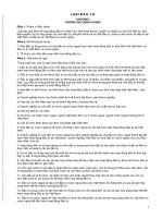
The relationship between investment and saving is
illustrated in Chart 1. Investment demand (I
0
) is nega-
tively dependent on the real interest rate, because a lower
real interest rate makes fixed investment more profit-
able. The saving curve (S
0
) is rising because households
are assumed to reduce current consumption relative to
future consumption when the real interest rate increases.
It is important to distinguish between preferred quanti-
ties ex ante and actual quantities ex post. Preferred sav-
ing ex ante may be different from preferred investment.
It is then up to the real interest rate to achieve a balance
so that these are equal ex post (point A on the chart).
Globally – or in a closed economy – saving is always
equal to investment ex post.
Changes in potential growth and the household rate
of time preference lead to permanent changes in saving
and investment behaviour and hence to changes in the
long-term equilibrium real interest rate. A higher invest-
ment preference shifts the demand curve outwards in
Chart 1 (from I
0

to I
1
). The new and higher real interest
rate level generates more saving, so that the increase
in investment demand is covered. A new adjustment
takes place at point B. One way of looking at this is that
when investment demand increases, the economy needs
a higher real interest rate in order not to overheat, and it
can take the higher real interest rate without dampening
the activity level. A higher saving preference shifts the
saving supply outwards (from S
0
til S
1
). A lower real
interest rate leads to higher investment, which accord-
ingly absorbs the increase in the saving supply. A new
adjustment takes place at point C. When the saving sup-
ply increases, the economy can take a lower real interest
rate without overheating, and it needs a lower real inter-
est rate to prevent a dampening of the activity level.
The Ramsey model is stylised and most useful as a
starting point for assessing long-term developments in
the real interest rate. The model indicates a long-term
relationship between potential growth and the real inter-
est rate.
3 A closer look at the neutral real
interest rate
Definition
The concept “neutral real interest rate” is generally asso-

ciated with the real interest rate level which implies that
monetary policy is neither expansionary nor contrac-
tionary. There is no definitive definition of the neutral
6
In the Ramsey model, the saving ratio is determined by consumers maximising their utility. The expression in equation (1) is based on a simplified assumption that the utility function is logarith-
mic. This simplification makes the discussion somewhat simpler without losing the central points of the model. Blanchard and Fisher (1989) and Romer (2001) provide a more in-depth discussion
of this question and the Ramsey model in general. Hammerstrøm and Lønning (2000) also provide a somewhat more detailed discussion.
7 Given the assumptions in footnote 6 it can be shown that MPC – v = r** = g + n + ρ, where MPC is the marginal productivity of capital (gross) and v is the depreciation rate of capital (Romer,
2001). If, for the sake of simplicity, we assume that households’ rate of time preference is zero, the net marginal productivity of capital (MPC – v) must be equal to the real interest rate, which in
turn must be equal to potential economic growth. The expression can be interpreted as an equilibrium condition. Suppose, for example, that the marginal return on capital increases as a result of
technological advances. The marginal return on capital is then higher than the real interest rate, which provides an incentive for increased investment. As a result, investment demand increases,
and the real interest rate rises.
Chart 1 Saving, investment and long-term real interest rate
Real interest rate
Saving (S), Investment (I)
S
0
S
1
I
1
I
0
B
A
C
r
B
r
A

r
C
E c o n o m i c B u l l e t i n 2 / 2 0 0 7
53
E c o n o m i c B u l l e t i n 2 / 2 0 0 7
54
real interest rate, and there are a number of approaches
to it in the literature.
Yellen (2005), president of the San Francisco Federal
Reserve, states: “Conceptually, policy can be deemed
“neutral” when the federal funds rate reaches a level
consistent with full employment of labor and capital
resources over the medium run.”
We accordingly define the neutral real interest rate as
the real interest rate level, which in the medium term is
consistent with a closed output gap. The output gap is
defined as the difference between actual and potential
output, which is the output level that is consistent with
stable inflation over time. Chart 2 illustrates a hypo-
thetical path for the real interest rate and the output gap.
The central bank sets the interest rate such that the mon-
etary policy objectives are expected to be achieved. In
the medium term, the output gap is expected to stabilise
at around zero.
8
The neutral real interest rate can change over time.
Yellen describes this as follows: “The value of [the
neutral rate] depends on the strength of spending – that
is, the aggregate demand for U S produced goods and
services. Aggregate demand, in turn, depends on a

number of factors. These include fiscal policy; the pace
of growth in our main trading partners; movements in
assets prices, such as stocks and housing, that influence
the propensity of households to save and spend; the
slope of the yield curve, which determines the level of
long-term interest rates associated with any given value
of the federal funds rate; and the pace of technological
change, which influences spending ”
Yellen is referring here to different disturbances to
the economy that may lead to changes in the neutral
real interest rate. Disturbances to the economy may
influence the prospects of closing the output gap in
the medium term. Positive demand shocks of a certain
duration tend to widen the output gap. To counteract
this, and ensure that the output gap stabilises at around
zero in the medium term, the real interest rate must
increase. This means that the neutral real interest rate has
increased. Similarly, negative demand shocks of a certain
duration will tend to reduce the output gap. To counteract
this, and stabilise the output gap at around zero in the
medium term, the real interest rate must be reduced. This
means that the neutral real interest rate has fallen.
The relationship between the long-term
equilibrium real interest rate and the
neutral real interest rate
Whereas the long-term equilibrium real interest rate is
determined by factors such as productivity, population
growth and long-term saving preferences, the neutral
real interest rate is additionally influenced by various
disturbances that influence the economy in the medium

term. Examples are temporary changes in fiscal policy
and in consumer and investment demand. The relation-
ship between the long-term equilibrium real interest rate
and the neutral real interest rate is illustrated in Chart 3.
The neutral real interest rate can be envisaged as mov-
ing around and towards the long-term equilibrium real
interest rate over time (in the absence of new shocks).
9
The relationship between the neutral and
the actual real interest rate
In the event of stickiness of wage and price formation,
the central bank can influence the real interest rate and
economic developments by changing the policy rate.
The real interest rate may therefore deviate from the
neutral level, depending on how the central bank seeks
to orient monetary policy. This in turn depends on the
central bank's trade-off between different objectives,
such as stable inflation on the one hand, and stable out-
put and employment on the other.
Chart 2 Output gap and real interest rate
Neutral real interest rate
Output gap stable around zero
Time
r*
0
Actual real interest rate
Output gap
8
“Medium term” is not clearly defined at the outset. To provide some idea of the time perspective, the medium term can probably be thought of as a horizon of from 1–2 years and up to 5–6 years.
“Medium term” may therefore be different from the central bank’s horizon for achieving the monetary policy objectives, such as that inflation shall be at a particular level.

9 New-Keynesian theory can be used to shed more light on this relationship. In these models, the neutral real interest rate is interpreted as the real interest rate that would have prevailed if wages
and prices had been flexible also in the short to medium term. In general, the neutral real interest rate will depend on all disturbances that influence the supply and demand side of the economy (see
Appendix 1 for a more detailed discussion).
Chart 3 Illustration of possible relationship between long-term
equilibrium real interest rate and neutral real interest rate over time
Time
Real interest rate
Long-term equilibrium real
interest rate
Neutral real interest rate
E c o n o m i c B u l l e t i n 2 / 2 0 0 7
In summary, the three real interest rate concepts are
related as follows:
•
Long-term equilibrium real interest rate: Determined
by economic fundamentals such as long-term saving
behaviour, productivity and population growth.
•
Neutral real interest rate: Determined by all the
disturbances to the economy that influence the pros-
pect of closing the output gap in the medium term.
These include the fundamentals that determine the
long-term equilibrium real interest rate, but also dis-
turbances of a more temporary nature.
•
Actual real interest rate: Determined by the central
bank’s desire to conduct an expansionary or con-
tractionary monetary policy. When economic distur-
bances occur, the central bank sets the real interest
rate lower or higher than the neutral level with a

view to stabilising the economy so that monetary
policy objectives are achieved.
4 The neutral real interest rate in a
small open economy
The definition of the neutral real interest rate – “the real
interest rate level, which in the medium term is consistent
with a closed output gap” – also holds for a small open
economy. However, a small open economy is heavily
influenced by global factors. One possible point of depar-
ture for discussing interest rates in a small open economy
is risk-adjusted uncovered interest rate parity:
(2) i
D
= i
G
+ (e
e
– e) + rp
In this equation, i
D
is the domestic interest rate, i
G
is
the global interest rate, e is the exchange rate, e
e
is the
expected future exchange rate and rp is a risk premium.
The exchange rate is defined as the number of units of
the domestic currency that must be paid for one unit
of the foreign currency. When the price of a foreign

currency is expected to rise, the domestic currency is
expected to depreciate, i.e., (e
e
– e) > 0.
10
When the risk premium is zero, uncovered interest rate
parity holds. The expected return on investing globally
(measured in domestic currency) is then equal to the
return on investment in the home country. If the expect-
ed return on global investment differs from the return
on domestic investment, investors will shift toward
investments yielding the highest returns. Suppose, for
example, that the global interest rate falls. Domestic
fixed-income securities will then be more attractive to
both domestic and foreign investors. Demand for them
will increase, leading to both lower domestic interest
rates and an appreciation of the domestic currency.
The risk premium does not have to be zero.
11
As a
result of factors relating to the risk premium, exchange
rate and expected exchange rate, global and domestic
interest rates do not necessarily move entirely in pace
with one another. Nevertheless, interest rate parity
provides a reasonable explanation for why domestic
interest rates are influenced by global interest rates: If
finical market participants anticipate large differences
in expected returns in different countries, they will tend
to make portfolio changes that reduce the difference in
expected return.

Normally the relationship between global and domes-
tic interest rates will be stronger for long-term rates than
for short-term rates (see Charts 4 and 5). Long-term
interest rates are largely determined by expected growth
and by inflation expectations, which do not necessarily
differ substantially across countries. Short-term rates
are largely determined by a country’s monetary policy,
which may differ depending on the cyclical phase of the
country’s economy at the time.
10
In equation (2) the exchange rate is expressed in logarithmic form.
11
If the risk premium is not zero, it means that investors are willing to hold both domestic and foreign fixed-income securities, even if the expected return on the two is different.
Chart 4 3-month money market rate. Monthly figures. Norway, the US,
the euro area and Sweden
0
2
4
6
8
2000 2001 2002 2003 2004 2005 2006
0
2
4
6
8
Norway
US
Euro area
Sweden

Source: EcoWin
Chart 5 10-year yield. Government bonds. Monthly figures.
Norway, the US, the euro area and Sweden
0
2
4
6
8
2000 2001 2002 2003 2004 2005 2006
0
2
4
6
8
Norway
US
Euro area
Sweden
Source: EcoWin
55
E c o n o m i c B u l l e t i n 2 / 2 0 0 7
56
Just as global nominal interest rates may influence
domestic nominal interest rates, global saving and
investment behaviour and the global neutral real inter-
est rate may influence the neutral real interest rate in a
small, open economy. There is no simple relationship
between the global neutral real interest rate and the neu-
tral real interest rate in a small, open economy. The rela-
tionship will depend on how the economies function,

and the disturbances to which they are exposed. Global
disturbances may have ripple effects for the demand
and supply sides of a small, open economy, and thereby
contribute to output deviating from potential output.
Disturbances arising in a small, open economy will not
normally affect economic developments in the rest of
the world. A detailed analysis of these relationships will
require a model of the global economy and the domestic
economy. We will confine ourselves here to pointing to
some mechanisms which may contribute to an under-
standing of how the neutral real interest rate in a small,
open economy can be influenced by global factors.
Our starting point is a stylised relationship between
demand for fixed investment and the supply of real
saving globally and at home, assuming unrestricted and
cost-free trading of goods and services. Movements of
capital between countries are disregarded in order to
highlight some central points which will also apply in
a pure barter economy. The analysis is then expanded
to include movements of capital between countries (a
portfolio theory approach).
Chart 6 shows demand for real investment and the
supply of real savings globally and domestically. The
small country cannot influence the global interest rate
(r*), and must take it as a given. This means that all
investment and saving in the small country take place at
the global real interest rate. It is initially assumed that
saving is equal to investment, both globally and domes-
tically (point A). This means that the balance of trade
is zero for both “countries”.

12
It is further assumed that
the real interest rate is the same as the neutral rate both
at home and abroad.
A higher global saving preference shifts the global
saving supply curve outwards (from S
*0
to S
*1
). This
pushes global real interest rates down (from r
*0
to r
*1
)
and increases global investment demand, which absorbs
the increase in the global saving supply. The domestic
real interest rate will then fall, providing an incentive
to reduce saving (point B’) and increase fixed invest-
ment (point B’’). The difference between investment
and saving is equal to the trade deficit. Output remains
equal to potential output in the small country because
the increase in investment demand is covered by higher
imports.
13
To provide a better understanding of the dynamics
in a small open economy when there is a preference
to increase global saving, the analysis is broadened to
include capital movements (see Chart 7). Initially, the
neutral global real interest rate is equal to the neutral

domestic real interest rate (r
1
). The global neutral real
interest rate is assumed to fall to r
2
.
• If the domestic interest rate remains unchanged at r
1
,
the difference against the global rate will increase.
This will contribute to an appreciation of the domestic
currency. The appreciation will dampen demand and
reduce the output gap in the medium term in the home
country. An unchanged real interest rate can therefore
not be an equilibrium: the neutral real interest rate
must have fallen. The question is, by how much.
• If the domestic real interest rate is reduced as much
as the global real interest rate (r
2
) , the interest rate
differential between them will remain unchanged. It
is then reasonable to assume that the nominal and
the real exchange rate will also remain unchanged.
However, a lower domestic real interest rate will
have an expansionary effect. Unless the entire
increase in demand is covered by imports, the output
gap will increase in the medium term. The export
and import pattern will change slowly over time,
while interest and exchange rates will adapt rapidly
12

From economic theory and national accounts we know that R=C+I+(A–B), where the letters stand for production, consumption, investment, exports and imports, in
that order. Moreover, S=R–C, where S is saving. It follows from this that S=I+(A–B), i.e. that a country can save through fixed investment or by having a balance of
trade surplus. When saving is equal to investment, the balance of trade is zero (for the sake of simplicity we do not distinguish here between the trade balance and the
current account).
13
In practice some frictions arise, as a result of which the domestic real interest rate will be different from the global rate. For example, a small open economy can prob-
ably not accumulate a trade deficit without having to pay a higher risk premium. It is commonly assumed that the risk premium – and accordingly the real interest rate
– increases with a country’s debt.
Chart 6 Effect of lower global neutral real interest rate. Real economic approach
Global Small, open economy
Real interest rate
I
S
r
*0
I
S
*0
Saving (S), Investment (I)
S
*1
Import
surplus
r
*1
B’’B’
A
Chart 7 Effect of lower global neutral real interest rate. Portfolio approach
r
1

r
2
Appreciation of the domestic currency
Negative output gap in the longer term
r > r*
r = r*
r
3
Real interest rate
Demand growth
Positive output gap in the
longer term r < r*
E c o n o m i c B u l l e t i n 2 / 2 0 0 7
to a new equilibrium in a world with well developed
capital markets. It therefore appears more realistic
to assume that a combination of a lower real inter-
est rate and a stronger real exchange rate is what is
required to stabilise the output gap in the medium
term in a world with free capital movements.
• It therefore appears reasonable that the new level
for the domestic neutral real interest rate should lie
somewhere between the old global level (r
1
) and the
new global level (r
2
), for example r
3
. A domestic real
interest rate fall from r

1
to r
3
will have an expansion-
ary effect and contribute to a larger output gap. The
fact that the interest rate differential is positive (r
3

> r
2
) contributes to strengthening the real exchange
rate and reducing the output gap. It is conceivable
that these effects are offsetting so that that the overall
monetary policy stance remains unchanged and con-
sistent with a closed output gap in the medium term.
5 Estimation of the long-term equi-
librium real interest rate and neutral
real interest rate
Potential growth and long-term equilib-
rium real interest rate
Potential growth may be of importance to both the
long-term equilibrium real interest rate and the neutral
real interest rate. Table 1 shows average growth and the
average real interest rate from1986 and 1994 for the G7
countries and Norway. The general picture is that aver-
age growth lies in a range from just under 2.5 per cent
to just over 3.0 per cent. The interval for the real interest
rate is somewhat larger.
Table 1 Growth and short-term real interest rate for the G7
countries and Norway*

G7 Norway
Growth Real interest rate Growth Real interest rate
1986–2006 2,6 2,5 2,4 4,6
1994–2006 2,5 1,6 3,1 3,0
* Growth is measured as average four-quarter growth over the period
in question. The real interest rate is a short-term nominal interest rate
deflated by consumer prices. The G7 countries are Canada, France,
Germany, Italy, Japan, the UK and the US.
Sources: EcoWin and Norges Bank
The European Central Bank (ECB) estimates potential
growth in the euro area to lie in the lower end of the
range, 2–2
1
/2 per cent
14
, while it is widely believed that
the growth potential in the US is somewhat higher, at
about 3 per cent.
15
In Norway, potential growth is esti-
mated at about 2
1
/2 per cent.
16
The estimates for poten-
tial growth and the long-term equilibrium real interest
rate are highly uncertain. The overall impression is that
for both Norway and the G7 countries, the long-term
equilibrium real interest rate normally appears to be
in a range around 2

1
/2–3
1
/2 per cent. Assigning a more
precise estimate would be to over-rate the methods and
possibilities available for estimating the long-term equi-
librium real interest rate.
Methods for estimating the neutral real
interest rate
There are a number of methods for assessing the neutral
real interest rate (see Giammarioli and Valla (2004) for
an overview). One possible estimate of the neutral real
interest rate is the average of historical real interest
rates. If the neutral real interest rate is constant over
time, an average of historical real interest rates over an
entire business cycle will provide an indication of the
level of the neutral real interest rate. The problem with
the method is that the neutral real interest rate cannot be
assumed to be constant over time. It can also be difficult
to decide when a business cycle starts and ends.
Other methods attempt to measure market participants’
expectations regarding future short-term real interest
rates. This is done by means of real return bonds, mar-
ket surveys (for example by Consensus Forecasts) and
by estimating market participants' future interest rate
expectations via market rates (implied rates
17
). The
shortcoming of these methods is, first, that they do not
necessarily capture market participants' actual interest

rate expectations, and second that market participants'
future interest rate expectations may deviate from the
neutral real interest rate.
One commonly used method for estimating the neu-
tral real interest rate is to specify an econometric model,
combine actual data and a priori assumptions about
developments in the unobservable variables (often other
unobservable variables, such as potential output and
equilibrium unemployment, are also included), and to
use the Kalman filter to estimate the neutral real inter-
est rate. The problem with the method is that the model
that forms the basis for the calculations is often highly
simplified compared with reality. The estimates are
generally sensitive to a number of technical choices in
the estimation process, and are therefore shrouded in
uncertainty.
The neutral real interest rate can also be estimated
using dynamic stochastic general equilibrium (DSGE)
models, which are often based on New-Keynesian the-
ory. In these models, the participants are forward-look-
ing, while the central bank sets the interest rate with a
view to stabilising inflation and output over time. Wages
and prices are sticky in the short term, but flexible in
the long term. If the assumption about sticky nominal
wages and prices is relaxed, the flexible price version of
14
See ECB (2005) and Trichet (2005).
15
See for example Financial Times (2006a, 2006b) and the IMF (2006).
16

This is Norges Bank’s estimate of potential mainland growth in Inflation Report 3/06.
17
For estimation and interpretation of implied rates, see Kloster (2000) and Myklebust (2005).
57
E c o n o m i c B u l l e t i n 2 / 2 0 0 7
58
the model emerges, i.e. the developments in economic
variables that would have occurred if all prices had been
flexible. In these models, the neutral real interest rate
is interpreted as the real interest rate that applies in the
“flexible price” version (see Appendix 1). This method
of estimating the neutral real interest rate is on the one
hand theoretically appealing, as there is a relationship
between the neutral real interest rate and other variables,
like the output gap, which is consistent with theory. This
is not necessarily the case with the other more “tradi-
tional” methods described above. On the other hand,
a model with quantified coefficients is required. The
model does not necessarily have to be true to reality.
The estimate of the neutral real interest rate is therefore
sensitive to the choice of model and the estimation
and calibration of the model’s parameters. For further
details, see Gali (2002) and Giammarioli and Valla
(2004). Amato (2005) discusses some differences in the
“flexible price” solution for the neutral real interest rate
and more traditional empirical methods.
It is clear from the above that there is no simple meth-
od for estimating the neutral real interest rate. A number
of methods exist, and there is uncertainty attached to all
of them. Nevertheless, the literature, in which a broad

range of different methods are used, can generally con-
tribute to providing an overall picture of the magnitude
of the neutral real interest rate.
Estimates of the global neutral real
interest rate
The ECB (2004) points out that many estimates of the
neutral real interest rate in the euro area lie in the interval
2–3 per cent, but also refers to the substantial uncertainty
associated with the estimates. The ECB argues that the
neutral real interest rate in the euro area may have fallen
in the past 10–15 years as a result of lower productivity
and population growth in the euro area, the elimination
of exchange rate risk within the euro area after the intro-
duction of a common currency, improved public finances
prior to the implementation of the common currency and
a fall in the inflation risk premium due to a fall in infla-
tion expectations to a stable, low level.
18
Giammarioli and Valla (2003) present arguments for
a gradual fall in the neutral real interest rate in the euro
area, from about 4 per cent in the mid-1990s to around
3 per cent in 2000. Cuaresma, Gnan and Ritzberger-
Gruenwald (2003) indicate that the neutral real interest
rate in the euro area has fallen somewhat since 2000,
and propose a level of around 2 per cent at the end of
2002. Garnier and Wilhelmsen (2004) also find that the
neutral real interest rate has fallen in recent years, both
in the euro area and in Germany. Goldman Sachs (2004)
maintains that the neutral real interest rate in the euro
area has fallen over the past 15 years, and estimates it at

around 2 per cent in October 2004.
Laubach and Williams (2003) estimate the neutral real
interest rate in the US from the early 1960s up to 2002.
They find that the neutral real interest rate has fallen
gradually over time. A possible explanation for this
trend may be a fall in the inflation risk premium. Aside
from the general fall in the long-term trend, Laubach
and Williams find that the neutral real interest rate was
temporarily low in the mid-1990s, but rose in the latter
half of this decade. A widely accepted explanation for
the latter is the high productivity growth (new economy
wave) of the latter half of the 1990s. In the first few
years of this century, the neutral real interest rate in
the US fell, which can be explained by the sharp fall in
equity prices and slower growth in these years. Laubach
and Williams estimate the neutral real interest rate in the
US at about 3 per cent in mid-2002. The OECD (2004)
updates the Laubach and Williams study, and finds that
the neutral real interest rate in the US may be just over
2 per cent at the end of 2004.
19
In a speech given in October 2004, Roger W. Ferguson
refers to a fall in US interest rates from 2001 to 2004,
and points out that even though short-term real inter-
est rates fell substantially, the neutral real interest rate
fell at the same time. Factors contributing to the fall in
the neutral real interest rate included: “ an unusual
hesitancy on the part of businesses to hire and spend
emerged in 2001 after the collapse of equity prices
and the restraint imposed on domestic consumers

from an increase in the cost of energy.”
20
Manrique and Manuel Marques (2004) estimate the
neutral real interest rate in the US and Germany from
the mid-1960s to the end of 2001. Their results for the
US are comparable with those of Laubach and Williams.
Whereas the neutral real interest rate rose somewhat in
the latter half of the 1990s, it fell in the years imme-
diately after the turn of the century. Towards the end
of 2001 it was estimated at about 2½ per cent. Amato
(2005) argues that the neutral real interest rate in both
the US and the euro area may be in the range 2½–2¾ per
cent, which is consistent with the estimates of the BIS
(2005). Goldman Sachs (2005) estimates the neutral real
interest rate in the US at about 2.5 per cent. Wu (2005)
argues that the neutral real interest rate in the US has
varied between 4 and 2 per cent since the 1960s and that
it was around 2½ per cent in early 2005.
The neutral real interest rate is also mentioned from
18 Uncertain future inflation may lead to an inflation risk premium and higher real interest rate. The nominal interest rate can be expressed as i = r
e
+ π
e
+ rp
π
+ rp
term
,
where i is the nominal interest rate, r
e

is the expected real interest rate, π
e
is expected inflation, rp
π
is an inflation risk premium and rp
term
is the term premium. While
the term premium reflects the extra expected return investors require for investing in fixed-income securities with a long maturity, the inflation risk premium reflects
the extra expected return they require because future inflation is uncertain. Uncertain future inflation makes the real value of investments uncertain. Investors may
require extra compensation – a risk premium – for this. As inflation fell in the 1980s and 1990s, so that inflation expectations became entrenched at a low and stable
level, it is reasonable to believe that the inflation risk premium also fell, which contributes to a lower real interest rate.
19 Laubach and Williams (2003) are the first to use the Kalman filter to estimate the neutral real interest rate, and the article is one of the most widely quoted works in
the empirical literature on the neutral real interest rate. A number of subsequent studies for both the US and other countries are based on the “Laubach and Williams
method”. The estimates are very uncertain and sensitive to a number of choices associated with the method. Ferguson (2004) therefore maintains, with reference to
Laubach and Williams’ estimates, that “ clearly, this estimate is not measured sufficiently precisely to be a useful guide to policy ”.
20 See Ferguson (2004). Ferguson was Vice Chairman of the US Federal Reserve Board from 1999–2006.
E c o n o m i c B u l l e t i n 2 / 2 0 0 7
59
time to time in the press. The Financial Times (2005)
refers to a neutral nominal policy rate (the federal funds
rate): “ generally seen as a range centred around 4¼
per cent , and the central bank’s presumed 1–2 per
cent comfort range based on the core personal consump-
tion expenditure measure ”. This implies a neutral real
interest rate of around 2.75 per cent. In an article of 12
July 2004, the same newspaper refers to Robert Parry,
former president of the San Francisco Federal Reserve,
who is of the opinion that an estimate of the neutral
real interest rate may be: “ the average for the real
federal funds since the 1960s of 2.5–3.5 per cent.” If

we take account of the widespread view that the neutral
real interest rate has fallen gradually during this period,
Parry’s lower limit may be a reasonable estimate.
There are also studies for other countries. Björksten
and Karagedikli (2003) and Lam and Tkacz (2004)
present arguments for a fall in the neutral real interest
rate in New Zealand and Canada, respectively. Brzoza-
Brzezina (2006) finds that the neutral real interest rate is
somewhat higher in Poland than in the US and the euro
area. Sveriges Riksbank (2006) finds that 3½–5 per cent
may be a reasonable range for the neutral nominal key
rate in Sweden.
Estimates of the neutral real interest rate
in Norway
We shall look more closely at the neutral real interest
rate in Norway. Chart 8 shows developments in infla-
tion, measured by changes in consumer prices and the
short-term real interest rate since 1987. The chart also
shows an estimate of long-term inflation expectations
since the early 1990s. It is reasonable to believe that,
as inflation became entrenched at a low level in the
1990s, long-term inflation expectations became simi-
larly entrenched. The long-term inflation expectations
are measured by average inflation up to the time when
the inflation target was introduced in March 2001 (about
2 per cent), thereafter by the inflation target of 2.5 per
cent. Low and stable inflation has probably contributed
to a permanent fall in the inflation risk premium and
accordingly the neutral level. In the past 10–12 years,
the real interest rate has largely ranged from just under

1 per cent to just over 6 per cent. High values for the
real interest rate indicate that it has been higher than the
neutral real interest rate, while low values indicate that
it has been lower than the neutral level.
Chart 9 shows implied long-term forward rates de-
flated by long-term inflation expectations. The starting
point for the calculation is nominal implied five-year
rates five years ahead, which is an estimate of market
participants’ expectations regarding the future nominal
interest rate. To the extent that implied rates are unaf-
fected by cyclical factors, they may reflect the expected
interest rate level when the output gap is closed in the
future. This measure of market participants’ expected
real interest rate five years ahead has ranged from just
over 1 per cent to about 4 per cent in the last 7–8 years.
In recent years it has fallen, and is now about 2 per cent.
As discussed above, implied interest rates do not neces-
sarily provide a reliable estimate of market participants’
interest rate expectations, and their expectations regard-
ing the future real interest rate may differ from the neu-
tral real interest rate. Implied interest rates, in particular,
may partly reflect cyclical factors and as a result not be
entirely in line with the interest rate level that is consist-
ent with a closed output gap in the medium term.
21
A Taylor rule can also be used as the starting point
for estimating the neutral real interest rate. A rule of
this kind says something about how the interest rate
should be set, depending on the size of the inflation gap
(inflation less the inflation target) and the output gap.

When both gaps are zero, the interest rate should be set
at the neutral rate. The constant in the Taylor rule can
therefore be interpreted as the neutral nominal interest
rate. We have estimated a Taylor rule for Norway for the
21
This is also pointed out by First Securities (2006).
Chart 8 Inflation measured by the consumer price index, long-term
inflation expectations and short-term real interest rate*. Norway.
Quarterly figures
-3
0
3
6
9
12
1986 1989 1992 1995 1998 2001 2004
-3
0
3
6
9
12
Inflation
Assumed long-term inflation expectations
Real interest rate
Source: EcoWin and Norges Bank
*3-month money market rate less annual inflation measured by the consumer
price index
Sources: EcoWin and Norges Bank
Chart 9 Inflation (CPI), long-term inflation expectations and implied

5-year rates 5 years ahead less long-term inflation expectations
-3
0
3
6
9
12
1986 1989 1992 1995 1998 2001 2004
-3
0
3
6
9
12
Inflation
Assumed long-term inflation expectations
Implied 5-year rates 5 years ahead
less long-term inflation expectations
period 1997–2006, in which the estimate of the neutral
nominal 3-month interest rate is just under 6 per cent.
When the inflation target of 2.5 per cent is subtracted,
this implies an estimated neutral real interest rate of
just over 3 per cent on average over the whole period.
Alternatively, the Taylor rule can be solved for the con-
stant for given values of the coefficients of inflation and
the output gap.
22
Measured in this way, the neutral real
interest rate has ranged in the last couple of years from
just under 2 per cent to just over 3 per cent (see Chart

10).
23
There is considerable uncertainty associated with
these methods. Central banks never set the interest rate
solely on the basis of a Taylor rule. In consequence,
mechanical calculation of the constant will not neces-
sarily produce a reliable estimate of the neutral real
interest rate. In Chart 10, for example, the estimated
neutral real interest rate around the peak in 2002/2003 is
clearly too high, and reflects the actual interest rate set-
ting rather than the level of the neutral real interest rate.
Chart 11 shows an estimate of the neutral real interest
rate in Norway which has been arrived at by specifying
a very simple econometric model and estimating the
neutral real interest rate by means of the Kalman filter.
The chart indicates that the neutral real interest rate
may now be less than 2½ per cent. For a more detailed
discussion of the method, see Appendix 2.
The methods used above do not provide an exact esti-
mate of the neutral real interest rate in Norway, which
we estimate will normally lie in the interval 2½–3½ per
cent. In recent times, with low real interest rates glo-
bally, we cannot exclude the possibility that it may be
even lower. In recent years, historical real interest rates
have moved around this range. Moreover, the methods
based on implied interest rates, the Taylor rule and the
Kalman filter are consistent with this level.
The estimates of the neutral real interest rate in
Norway have been reduced over time. On the basis of
historical data, Hammerstrøm and Lønning (2000) find

that 3–4 per cent may be a reasonable range for the
neutral real interest rate in Norway. In view of develop-
ments in estimates for the global neutral real interest
rate and different estimates for the neutral real inter-
est rate in Norway, it appears reasonable to revise this
somewhat downward. A lower inflation risk premium,
in particular, may have contributed to this (see footnote
18). After a period of falling inflation in the 1980s, it
took some years before inflation became entrenched
at a low and stable level (see Chart 8). From the mid-
1990s, it is reasonable to believe that the inflation risk
premium has been considerably lower than in the 1980s
and early 1990s. This points towards a lower neutral
real interest rate.
6 Conclusions
Whereas the long-term real interest rate is determined
by economic fundamentals such as potential growth and
private saving behaviour, the neutral real interest rate
is additionally affected by disturbances of a more tem-
porary nature which influence the supply and demand
sides of the economy.
The neutral real interest rate can be defined as “the real
interest rate level which in the medium term is consistent
with a closed output gap”. Protracted disturbances to the
economy may affect the prospects of closing the output
gap in the medium term. For example, expansionary
shocks will tend to widen the output gap. This means that
22
This method is used by Sveriges Riksbank (2006).
23 The estimated Taylor rule is given by i

3M
= 5,7 + 2,2 (π – π*) + 0,3 (Y–Y*), where i
3M
, (π – π*) and (Y–Y*) are the three-month nominal money market rate, the
inflation gap and the output gap, respectively. In order to provide a sufficiently long period for estimating the equation, we have used quarterly data since 1997, i.e. be-
fore inflation targeting was introduced in March 2001. The starting point was chosen partly because it was “from this point in time [January 1997] that daily quotations
and month-to-month variations in the exchange rate show that the krone is floating.” (Gjedrem, 2000). The output gap coefficient is not significantly different from
zero, and sensitive to the estimation period that has been chosen. The other coefficients are significantly different from zero. The magnitudes of the coefficients appear
reasonable and are in line with estimates for other countries. In the calculations upon which Chart 10 is based, the inflation gap coefficient is 1.5, while the output gap
coefficient is 0.5. These are the same coefficients as used by Taylor (1993).
Chart 10 Short-term real interest rate* and estimated neutral real interest
rate based on the constant in a Taylor rule. Norway. Quarterly figures
0
2
4
6
8
1997 1998 1999 2000 2001 2002 2003 2004 2005 2006
0
2
4
6
8
Short-term real interest rate
Neutral real interest rate
based on Taylor rule
Sources: EcoWin and Norges Bank
*3-month money market rate less annual inflation measured by the consumer
price index
Chart 11 Short-term real interest rate* and estimated neutral real

interest rate based on a Kalman filter
0
2
4
6
8
1997 1998 1999 2000 2001 2002 2003 2004 2005 2006
0
2
4
6
8
Short-term real interest rate
Neutral real interest rate
based on Kalman filter
Sources: EcoWin and Norges Bank
*3-month money market rate less annual inflation measured by the consumer
price index
E c o n o m i c B u l l e t i n 2 / 2 0 0 7
60
the neutral real interest rate has increased. The neutral
real interest rate may deviate from the long-term equili-
brium real interest rate, but will vary and, in the absence
of new shocks, move towards the long-term equilibrium
real interest rate over time.
Because of free movements of capital between countri-
es, the interest rates in a small open economy, including
the neutral rate, are dependent on global interest rates.
However, there is no simple relationship between the
global neutral real interest rate and the neutral real inte-

rest rate in a small, open economy. The relationship will
depend on how the economies function, and the shocks to
which they are exposed. Global shocks may have ripple
effects for the demand and supply sides of a small, open
economy – which may affect the prospects of closing the
output gap in the medium term.
In a small, open economy, exchange rate factors may
influence the neutral real interest rate. It is the overall
orientation of monetary policy – the combination of the
real interest rate and the real exchange rate – which is
decisive for economic activities and hence for the pro-
spects of closing the output gap in the medium term. In
isolation, a stronger exchange rate will dampen economic
activity. The prospects of closing the output gap in the
medium term must therefore be assessed in the light of
the effect that assumed interest rate movements abroad
and in Norway have on the exchange rate.
There are several methods for estimating the neutral
real interest rate, but there is substantial uncertainty
attached to all of them. Nevertheless, a broad spectrum of
methods can provide a picture of the range in which the
neutral real interest rate lies. An overall evaluation implies
that a range of around 2½–3½ per cent may normally be
regarded as covering both the long-term equilibrium real
interest rate and the neutral real interest rate in Norway.
In recent times, with low real interest rates globally, we
cannot exclude the possibility that the neutral real inte-
rest rate in Norway may be even lower. The neutral real
interest rate, both globally and in Norway, has probably
fallen compared with the 1980s and the first half of the

1990s. One reason for this is probably lower inflation
risk premia as inflation and inflation expectations have
become entrenched at a low and stable level.
Appendix 1. New-Keynesian theory
on the neutral real interest rate
In New-Keynesian models, the output gap is interpreted
as the difference between overall output and the level of
output that is consistent with flexible wages and prices
(hereafter called potential output).
24
The neutral real
interest rate can thus be interpreted as the real interest
rate that applies when wages and prices are flexible. A
strength of this definition is that there is a theoretically
consistent relationship between the neutral real interest
rate and other variables in the economy, such as the out-
put gap. A weakness is that the neutral real interest rate
in such models is sensitive to the model specification.
Woodford (2003) has pointed out that it may be optimal
in terms of welfare to use monetary policy to steer the
economy towards equilibrium with flexible prices.
25
Developments in the economy based on a New-
Keynesian model can be expressed by two equations,
one for the output gap, x
t
(the IS curve), and one for
inflation (the Phillips curve), π
t
, see equations (1) and

(2) respectively.
(1) x
t
= E
t
x
t+1
– σ (i
t
– E
t
π
t+1
– r
t
*)
(2)
π
t
= β E
t
π
t+1
+ κ x
t
The IS curve is based on the Euler equation for opti-
mal adaptation of private consumption over time, where
i
t
is the short-term nominal interest rate and E

t
π
t+1
is
expected inflation in the next period. The coefficient
(σ) expresses the intertemporal substitution elastic-
ity, i.e. how much consumers are willing to postpone
consumption if the real interest rate increases by one
percentage point. The difference (i
t
– E
t
π
t+1
) expresses
the short-term real interest rate (ex ante), while r
t
* is the
neutral real interest rate. Output depends one-to-one on
expected output, because households want to smooth con-
sumption over time. When the real interest rate is higher
than the neutral real interest rate or is expected to be in the
future, this will contribute to reduced consumption and a
smaller output gap. The Phillips curve is based on optimal
wage and price setting. The coefficient β can be interpreted
as enterprises’ discount factor, which is normally assumed
to be close to 1. When the output gap increases, it adds
to pressure on wages and prices because wage earners
demand higher real wages for working more (because
κ > 0), and enterprises will increase prices because pro-

duction costs are assumed to increase at the margin.
In the short and medium term, monetary policy can
be used to stabilise developments in output and prices.
As a result of the implied and explicit costs associated
with changes in prices and wages, it may take time
before economic disturbances feed fully through to
prices and wages. By adjusting the nominal interest rate
(i
t
) and having a rule for how the interest rate should be
adjusted in the future, the central bank can influence the
real interest rate and market participants' expectations.
If, however, wages and prices are fully flexible, the cen-
tral bank has no part to play in stabilisation policy. The
reason is that a change made by the central bank in the
nominal interest rate will lead to an equivalent change
in expected inflation, so that the real interest rate is not
affected. The real interest rate will thus always be equal
to the neutral real interest rate when prices and wages
are flexible.
E c o n o m i c B u l l e t i n 2 / 2 0 0 7
61
24 For a more in-depth account of New-Keynesian models, see Gali (2002) and Holmsen and Røisland (2006.
25 Adjusted for so-called “inefficient” shocks.
In this model, disturbances to the supply and
demand sides of the economy lead to changes in the
neutral real interest rate. Thus disturbances that lead to
an increase in the neutral real interest rate imply that
monetary policy may be perceived as expansionary. It
may therefore be necessary to increase the policy rate in

order to avoid pressure on wages and prices. The neutral
real interest rate can be written (see Gali, 2002)
26
:
(3) r
t
* = ρ + ρ
a
Δa
t
+ (1 – ψ
g
)(1 – ρ
g
)g
t
The neutral real interest rate can be divided into three
components:
•
Household demand/discount factor (ρ): If house-
holds place a high value on consumption now,
relative to consumption in the future, this discount
factor will be higher. A higher real interest rate will
then be necessary to ensure that overall demand is
not higher than potential output.
•
Productivity growth

(Δa
t

): When productivity growth
increases, so does the neutral real interest rate. The
persistence of a productivity growth shock depends
on ρ
a
(0<ρ
a
<1). Over time, increased productiv-
ity means increased output and income. Since the
households in this model prefer to smooth their con-
sumption over time, they will increase consumption
immediately when their lifetime income increases.
The real interest rate will therefore have to rise to
ensure that demand does not increase more than
potential output. The more persistent the produc-
tivity growth shock is (ρ
a
is higher), the more the
neutral real interest rate will increase. It follows from
this that a one-off change in the productivity level
(ρ
a
= 0) will not change the neutral real interest rate.

Empirically, however, there is little to indicate that
consumption changes suddenly as a result of, for exam-
ple, a change in productivity growth. The model above
can be expanded to include an assumption of habit per-
sistence in consumption.
27

This means that consumption
and the neutral real interest rate will increase less in
connection with a higher lifetime income than without
such a condition. If productivity growth increases while
habit formation remains strong, the neutral real interest
rate may fall to motivate households to increase their
demand as much as potential output. Otherwise there
will be idle economic resources.
• Demand shock (g
t
): When public authorities increase
their demand, this also contributes to a rise in the
neutral real interest rate. If the demand shock is
permanent (ρ
g
approaches 1), the real interest rate
increases less. The reason is a condition in this
model relating to balanced government budgets.
Permanently increased public sector demand means
higher taxation, lower household lifetime income,
and hence lower private consumption.
If the labour market is not very flexible (
ψ
g

is low), the labour supply and hence potential
output will only increase slightly when public sec-
tor demand increases. The real interest rate must
accordingly increase more to prevent total demand
from being higher than potential output.

The neutral real interest rate will therefore depend on
both short-term and long-term disturbances that influ-
ence the supply and demand side of the economy. The
above model can be expanded to include fixed invest-
ment and capital, but this will not have any significant
impact on the qualitative results.
Appendix 2. Estimating the neutral
real interest rate with a Kalman filter
The neutral real interest rate cannot be observed. A
method frequently used to estimate unobservable vari-
ables is the Kalman filter. By combining actual data and
a priori assumptions about developments in unobservable
variables, the Kalman filter provides estimates of the
latter. The neutral real interest rate is defined as the real
interest rate level which is consistent in the medium term
with a closed output gap. According to economic theory,
the neutral real interest rate will depend on unobservable
variables such as time preferences and growth in poten-
tial output. Empirical studies seek to use these relation-
ships to estimate the neutral real interest rate at the same
time as other unobservable variables (see for example
Laubach and Williams (2003), Garnier and Wilhelmsen
(2004) and Larsen and McKeown (2004)).
In this article, we use the Kalman filter to estimate the
neutral real interest rate with a highly simplified econo-
mic model as the starting point. First, we assume that the
real interest rate (r
t
) can be split into a trend component
(r

t
*) and a cyclical component (e
t
) (see equation (1)):
(1) r
t
= r
t
*
+ e
t
where e
t
~ N(0, σ
e
2
)
The trend component is defined here as the neutral real
interest rate. We furthermore assume that the neutral
real interest rate depends on a constant (μ), which can
be interpreted as a long-term equilibrium real interest
rate, and disturbances (z
t
) which cause the neutral real
interest rate to deviate from the long-term equilibrium
real interest rate. The disturbances are assumed to fol-
low an AR1 process, i.e. they depend on the disturban-
ces in the previous period and any new shocks in the
current period (ε
t

).
(2) r
t
* = μ + z
t

(3) z
t
= ρz
t–1
+ ε
t
where ε
t
~ N(0, σ
ε
2
)
These three equations can be used alone to estimate the
neutral real interest rate and can thus be regarded as a
E c o n o m i c B u l l e t i n 2 / 2 0 0 7
62
26 For the sake of simplicity, we assume here that σ = 1 in equation (1), which is in line with empirical calculations. Population growth is not taken into account.
27 See inter alia Fuhrer (2000) for a brief overview of empirical and theoretical studies of habit formation in consumption, and for a presentation of the consequences for
the Euler equation of expanding the household utility function to include this habit formation.
one-sided Hodrick-Prescott filter, because the filter does
not use information about the real interest rate ahead in
time to estimate the real interest rate today. However, we
also want to use information about a possible economic
relationship to estimate the neutral real interest rate and

assume that the output gap (x
t
) depends on the real inte-
rest rate gap (r
t
– r
t
*) as follows:
(4) x
t
= αx
t–1
– β(r
t–1
– r*
t–1
) + η
t
where η
t
~ N(0, σ
η
2
)
This equation is a simplified version of the IS curve in
Norges Bank's macroeconomic model (see Husebø et al.
(2004)). By setting up these equations in “state-space”
format, we can estimate the parameters (ρ, α and β), the
standard deviation of the shocks e
t

, ε
t
and η
t
and calculate
the neutral real interest rate.
28
We take the output gap
from Inflation Report 3/06 as given, and therefore do not
estimate this variable. We place restrictions on the variance
of the shocks (σ
η
2
=2.5, σ
e
2
=0.02 and σ
ε
2
=0.02) to ensure
a relatively smooth path for the neutral real interest rate.
These restrictions also contribute to the neutral real inte-
rest rate being influenced by both actual developments in
the real interest rate and the economic relationship (4).
Without these restrictions, the neutral real interest rate
has a tendency to be estimated as equal to the actual real
interest rate or the long-term equilibrium real interest
rate. This is because the model (1)–(4) is very simple.
The long-term equilibrium real interest rate (μ) is assu-
med here to be constant over time and is set at 2.5, and

can be regarded as a measure of underlying productivity
growth in the Norwegian economy.
Table 1 Parameter estimates
Parameter Estimate Standard deviation
α 0.97 0.006
β 0.17 0.005
ρ 0.99 0.001
The parameter estimates for the period 1981 Q1 – 2006
Q3 are shown in Table 1. They show that the output gap
is strongly dependent on the output gap in the previous
period, and that the real interest rate gap has a negative
impact on the output gap. The coefficient ρ is approxi-
mately equal to 1, which means that developments in the
neutral real interest rate can be regarded as a “random
walk”, i.e. that changes in the neutral real interest rate are
permanent. However, this may be because the model that
has been used is too simple. The estimates of the neutral
real interest rate are shown in Chart 11.
References
Amato, J. D. (2005): “The role of the natural rate of
interest in monetary policy”, Bank for International
Settlements, Working Papers, 171
BIS (2005): “Overview: low yields in robust economies”,
Bank for International Settlements, Quarterly Review,
March 2005
Björksten, N. and Ö. Karagedikli (2003): “Neutral
real interest rates revisited”, Reserve Bank of New
Zealand Bulletin, vol. 66, no. 3
Blanchard, O. J. and S. Fischer (1989): Lectures on
Macroeconomics, MIT Press

Blinder, A. S. (1998): Central banking in theory and
practice, MIT Press
Brzoza-Brzezina, M. (2006): “The information content of
the neutral rate of interest”, Economics of Transition
14, 391–412
Cueresma, J. C., E. Gnan and D. Ritzenberger-Gruenwald
(2003): “Searching for the natural rate of inte-
rest: a euro-area perspective”, Working Paper 84,
Österreichische Nationalbank
ECB (2004): “The natural real interest rate in the euro
area”, Monthly Bulletin, May/04, see www. ecb.int
ECB (2005): “Trends in euro area potential output
growth”, Monthly Bulletin July/05, see www. ecb.int
Ferguson, R. W. (2004): “Equilibrium real interest rate
– theory and application”. Speech, see www.federal-
reserve.gov
Financial Times (2005): “Fed thinking points to measu-
red rate rises this year”, 19 January
Financial Times (2006a): “Inflation worry as Fed hopes
for soft landing”, 20 July
Financial Times (2006b): “Complications on the way to
a soft landing”, 13 September
First Securities ASA (2006): “Makro morgenrapport”
(Macro morning report), 29 June, see www.first.no
Fuhrer, J. C. (2000): “Habit Formation in Consumption
and Its Implications for Monetary-Policy Models”,
The American Economic Review, Vol. 90, no. 3 June
E c o n o m i c B u l l e t i n 2 / 2 0 0 7
63
28 The calculations were carried out using the program Eviews.

E c o n o m i c B u l l e t i n 2 / 2 0 0 7
64
Gali, J. (2002): “New perspectives on monetary policy,
inflation, and the business cycle”, NBER, Working
Paper 8786, also published in Advances in economic
theory, edited by Dewatripont, M., L. Hansen and S.
Turnovsky, vol. III, 151–197, Cambridge University
Press 2003
Garnier, J. and B. R. Wilhelmsen (2005): “The natural
real interest rate and the output gap in the euro area:
a joint estimation”, European Central Bank, Working
Paper 546
Giammarioli, N. and N. Valla (2003): “The natural real
rate of interest in the euro area”, European Central
Bank, Working Paper 233
Giammarioli, N. and N. Valla (2004): “The natural real
interest rate and monetary policy: a review”, Journal
of Policy Modelling, 26, 641–660
Gjedrem, S. (2000): “Economic perspectives”. Annual
Address 2000. See www.norges-bank.no
Goldman Sachs (2004): Euroland Weekly Analyst, 04/44
Goldman Sachs (2005): US Economic Analyst, 05/01
Hammerstrøm, G. and I. Lønning (2000): “Kan vi tall-
feste den nøytrale realrenten?” (Can we quantify the
neutral real interest rate?), Penger og Kreditt 2/2000,
Norges Bank, see www.norges-bank.no
Holmsen, A. and Ø. Røisland (2006): “Hva har ny-keyne-
siansk teori betydd for pengepolitikken?” (What has
New-Keynesian theory meant for monetary policy?),
Økonomisk forum, no. 6

Husebø, T. A., S. McCaw, K. Olsen and Ø. Røisland
(2004): “A small calibrated macro model to sup-
port inflation targeting at Norges Bank”, Staff Memo
2004/3, Norges Bank
IMF (2006): World Economic Outlook, September 2006,
see www.imf.org
Kloster, A. (2000): “Estimating and interpreting interest
rate expectations”, Economic Bulletin 3/2000, Norges
Bank, see www.norges-bank.no
Myklebust, G. (2005): “Documentation of the method
used by Norges Bank for estimating implied forward
rates”, Staff Memo 2005/11, see www.norges-bank.no
Lam, J. P. and G. Tkacz (2004): “Estimating policy-
neutral interest rates for Canada using a dynamic
stochastic general-equilibrium framework”, Working
Paper 9, Bank of Canada
Larsen, J. D. J. and J. McKeown (2004): “The informa-
tional content of empirical measures of real interest
rate and output gaps for the United Kingdom”,
Working Paper 224, Bank of England
Laubach, T. and J. C. Williams (2003): “Measuring the
natural rate”, The Review of Economics and Statistics,
85(4), 1063:1070
Manrique, M. and J. M. Marques (2004): “An empiri-
cal approximation of the natural rate of interest and
potential growth”, Working Paper 0416, Banco de
Espana
OECD (2004): Economic Outlook, vol. 76
Sveriges Riksbank (2006): “What is a normal level for
the repo rate?”, Inflation Report 2/2006, www.riks-

banken.se
Romer, D. (2001): Advanced Macroeconomics,
McGrawHill
Taylor, J. B. (1993): “Discretion versus policy rules in
practice”, Carnegie-Rochester Conference Series on
Public Policy 39, pp. 195–214
Trichet, J. C. (2005): Interview with the Irish Times,
Le Figaro, El Mundo and Frankfurter Allgemeine
Zeitung, see www. ecb.int
Yellen, J. L. (2005): “President’s speech: Update in the
US Economy”. Speech, see www.frbsf.org
Wicksell, K. (1907): “The Influence of the Rate of
Interest on Prices”, Economic Journal, 17, June
Woodford, M. (2003): Interest & Prices. Princeton
University Press
Wu, T. (2005): “Estimating the neutral real interest rate in
real time”, FRBSF Economic Letter, 2005/27