Tài liệu Đề tài " On the K2 of degenerations of surfaces and the multiple point formula " pptx
Bạn đang xem bản rút gọn của tài liệu. Xem và tải ngay bản đầy đủ của tài liệu tại đây (1.02 MB, 62 trang )
Annals of Mathematics
On the K2 of
degenerations of surfaces
and the multiple point
formula
By A. Calabri, C. Ciliberto, F. Flamini, and R.
Miranda*
Annals of Mathematics, 165 (2007), 335–395
On the K
2
of degenerations of surfaces
and the multiple point formula
By A. Calabri, C. Ciliberto, F. Flamini, and R. Miranda*
Abstract
In this paper we study some properties of reducible surfaces, in particular
of unions of planes. When the surface is the central fibre of an embedded flat
degeneration of surfaces in a projective space, we deduce some properties of
the smooth surface which is the general fibre of the degeneration from some
combinatorial properties of the central fibre. In particular, we show that there
are strong constraints on the invariants of a smooth surface which degener-
ates to configurations of planes with global normal crossings or other mild
singularities.
Our interest in these problems has been raised by a series of interesting
articles by Guido Zappa in the 1950’s.
1. Introduction
In this paper we study in detail several properties of flat degenerations of
surfaces whose general fibre is a smooth projective algebraic surface and whose
central fibre is a reduced, connected surface X ⊂ P
r
, r 3, which will usually
be assumed to be a union of planes.
As a first application of this approach, we shall see that there are strong
constraints on the invariants of a smooth projective surface which degener-
ates to configurations of planes with global normal crossings or other mild
singularities (cf. §8).
Our results include formulas on the basic invariants of smoothable sur-
faces, especially the K
2
(see e.g. Theorem 6.1).
These formulas are useful in studying a wide range of open problems, such
as what happens in the curve case, where one considers stick curves, i.e. unions
of lines with only nodes as singularities. Indeed, as stick curves are used to
*The first two authors have been partially supported by E.C. project EAGER, contract n.
HPRN-CT-2000-00099. The first three authors are members of G.N.S.A.G.A. at I.N.d.A.M.
“Francesco Severi”.
336 A. CALABRI, C. CILIBERTO, F. FLAMINI, AND R. MIRANDA
study moduli spaces of smooth curves and are strictly related to fundamen-
tal problems such as the Zeuthen problem (cf. [20] and [35]), degenerations of
surfaces to unions of planes naturally arise in several important instances, like
toric geometry (cf. e.g. [2], [16] and [26]) and the study of the behaviour of
components of moduli spaces of smooth surfaces and their compactifications.
For example, see the recent paper [27], where the abelian surface case is con-
sidered, or several papers related to the K3 surface case (see, e.g. [7], [8] and
[14]).
Using the techniques developed here, we are able to prove a Miyaoka-Yau
type inequality (see Theorem 8.4 and Proposition 8.16).
In general, we expect that degenerations of surfaces to unions of planes will
find many applications. These include the systematic classification of surfaces
with low invariants (p
g
and K
2
), and especially a classification of possible
boundary components to moduli spaces.
When a family of surfaces may degenerate to a union of planes is an open
problem, and in some sense this is one of the most interesting questions in the
subject. The techniques we develop here in some cases allow us to conclude
that this is not possible. When it is possible, we obtain restrictions on the
invariants which may lead to further theorems on classification, for example,
the problem of bounding the irregularity of surfaces in P
4
.
Other applications include the possibility of performing braid monodromy
computations (see [9], [29], [30], [36]). We hope that future work will include
an analysis of higher-dimensional analogues to the constructions and computa-
tions, leading for example to interesting degenerations of Calabi-Yau manifolds.
Our interest in degenerations to unions of planes has been stimulated by
a series of papers by Guido Zappa that appeared in the 1940–50’s regarding in
particular: (1) degenerations of scrolls to unions of planes and (2) the computa-
tion of bounds for the topological invariants of an arbitrary smooth projective
surface which degenerates to a union of planes (see [39] to [45]).
In this paper we shall consider a reduced, connected, projective surface X
which is a union of planes — or more generally a union of smooth surfaces —
whose singularities are:
• in codimension one, double curves which are smooth and irreducible along
which two surfaces meet transversally;
• multiple points, which are locally analytically isomorphic to the vertex
of a cone over a stick curve, with arithmetic genus either zero or one,
which is projectively normal in the projective space it spans.
These multiple points will be called Zappatic singularities and X will be called
a Zappatic surface. If moreover X ⊂ P
r
, for some positive r, and if all its
irreducible components are planes, then X is called a planar Zappatic surface.
THE K
2
OF DEGENERATIONS OF SURFACES
337
We will mainly concentrate on the so called good Zappatic surfaces, i.e.
Zappatic surfaces having only Zappatic singularities whose associated stick
curve has one of the following dual graphs (cf. Examples 2.6 and 2.7, Defini-
tion 3.5, Figures 3 and 5):
R
n
: a chain of length n, with n 3;
S
n
: a fork with n − 1 teeth, with n 4;
E
n
: a cycle of order n, with n 3.
Let us call R
n
-, S
n
-, E
n
-point the corresponding multiple point of the Zappatic
surface X.
We first study some combinatorial properties of a Zappatic surface X
(cf. §3). We then focus on the case in which X is the central fibre of an
embedded flat degeneration X→∆, where ∆ is the complex unit disk and
where X⊂∆ × P
r
, r 3, is a closed subscheme of relative dimension two.
In this case, we deduce some properties of the general fibre X
t
, t = 0, of the
degeneration from the aforementioned properties of the central fibre X
0
= X
(see §§4, 6, 7 and 8).
A first instance of this approach can be found in [3], where we gave some
partial results on the computation of h
0
(X, ω
X
), when X is a Zappatic surface
with global normal crossings and ω
X
is its dualizing sheaf. This computation
has been completed in [5] for any good Zappatic surface X. In the particular
case in which X is smoothable, namely if X is the central fibre of a flat de-
generation, we prove in [5] that h
0
(X, ω
X
) equals the geometric genus of the
general fibre, by computing the semistable reduction of the degeneration and
by applying the well-known Clemens-Schmid exact sequence (cf. also [31]).
In this paper we address two main problems.
We will first compute the K
2
of a smooth surface which degenerates to a
good Zappatic surface; i.e. we will compute K
2
X
t
, where X
t
is the general fibre
of a degeneration X→∆ such that the central fibre X
0
is a good Zappatic
surface (see §6).
We will then prove a basic inequality, called the Multiple Point Formula
(cf. Theorem 7.2), which can be viewed as a generalization, for good Zappatic
singularities, of the well-known Triple Point Formula (see Lemma 7.7 and cf.
[13]).
Both results follow from a detailed analysis of local properties of the total
space X of the degeneration at a good Zappatic singularity of the central
fibre X.
We apply the computation of K
2
and the Multiple Point Formula to prove
several results concerning degenerations of surfaces. Precisely, if χ and g de-
note, respectively, the Euler-Poincar´e characteristic and the sectional genus of
the general fibre X
t
, for t ∈ ∆ \{0}, then:
338 A. CALABRI, C. CILIBERTO, F. FLAMINI, AND R. MIRANDA
•
•
•
•
•
•
•
•
•
•
•
•
•
(a) (b)
Figure 1:
Theorem 1 (cf. Theorem 8.4). Let X→∆ be a good, planar Zappatic
degeneration, where the central fibre X
0
= X has at most R
3
-, E
3
-, E
4
- and
E
5
-points. Then
K
2
8χ +1− g.(1.1)
Moreover, the equality holds in (1.1) if and only if X
t
is either the Veronese
surface in P
5
degenerating to four planes with associated graph S
4
(i.e. with
three R
3
-points, see Figure 1.a), or an elliptic scroll of degree n 5 in P
n−1
degenerating to n planes with associated graph a cycle E
n
(see Figure 1.b).
Furthermore, if X
t
is a surface of general type, then
K
2
< 8χ − g.
In particular, we have:
Corollary (cf. Corollaries 8.10 and 8.12). Let X be a good, planar
Zappatic degeneration.
(a) Assume that X
t
, t ∈ ∆ \{0}, is a scroll of sectional genus g 2. Then
X
0
= X has worse singularities than R
3
-, E
3
-, E
4
- and E
5
-points.
(b) If X
t
is a minimal surface of general type and X
0
= X has at most R
3
-,
E
3
-, E
4
- and E
5
-points, then
g 6χ +5.
These improve the main results of Zappa in [44].
Let us describe in more detail the contents of the paper. Section 2 contains
some basic results on reducible curves and their dual graphs.
In Section 3, we give the definition of Zappatic singularities and of (planar,
good) Zappatic surfaces. We associate to a good Zappatic surface X a graph
G
X
which encodes the configuration of the irreducible components of X as well
as of its Zappatic singularities (see Definition 3.6).
In Section 4, we introduce the definition of Zappatic degeneration of sur-
faces and we recall some properties of smooth surfaces which degenerate to
Zappatic ones.
THE K
2
OF DEGENERATIONS OF SURFACES
339
In Section 5 we recall the notions of minimal singularity and quasi-minimal
singularity, which are needed to study the singularities of the total space X
of a degeneration of surfaces at a good Zappatic singularity of its central fibre
X
0
= X (cf. also [23] and [24]).
Indeed, in Section 6, the local analysis of minimal and quasi-minimal
singularities allows us to compute K
2
X
t
, for t ∈ ∆ \{0}, when X
t
is the general
fibre of a degeneration such that the central fibre is a good Zappatic surface.
More precisely, we prove the following main result (see Theorem 6.1):
Theorem 2. Let X→∆ be a degeneration of surfaces whose central fibre
is a good Zappatic surface X = X
0
=
v
i=1
X
i
.LetC
ij
:= X
i
∩ X
j
be a smooth
(possibly reducible) curve of the double locus of X, considered as a curve on
X
i
, and let g
ij
be its geometric genus,1 i = j v.Letv and e be the
number of vertices and edges of the graph G
X
associated to X.Letf
n
, r
n
, s
n
be the number of E
n
-, R
n
-, S
n
-points of X, respectively. If K
2
:= K
2
X
t
, for
t =0,then:
K
2
=
v
i=1
K
2
X
i
+
j=i
(4g
ij
− C
2
ij
)
− 8e +
n
3
2nf
n
+ r
3
+ k(1.2)
where k depends only on the presence of R
n
- and S
n
-points, for n 4, and
precisely:
n
4
(n − 2)(r
n
+ s
n
) k
n
4
(2n − 5)r
n
+
n − 1
2
s
n
.(1.3)
In the case that the central fibre is also planar, we have the following:
Corollary (cf. Corollary 6.4). Let X→∆ be an embedded degeneration
of surfaces whose central fibre is a good, planar Zappatic surface X = X
0
=
v
i=1
Π
i
. Then:
K
2
=9v − 10e +
n
3
2nf
n
+ r
3
+ k(1.4)
where k is as in (1.3) and depends only on the presence of R
n
- and S
n
-points,
for n 4.
The inequalities in the theorem and the corollary above reflect deep geo-
metric properties of the degeneration. For example, if X→∆ is a degeneration
with central fibre X a Zappatic surface which is the union of four planes hav-
ing only an R
4
-point, Theorem 2 states that 8 K
2
9. The two values
of K
2
correspond to the fact that X, which is the cone over a stick curve
C
R
4
(cf. Example 2.6), can be smoothed either to the Veronese surface, which
has K
2
= 9, or to a rational normal quartic scroll in P
5
, which has K
2
=8
340 A. CALABRI, C. CILIBERTO, F. FLAMINI, AND R. MIRANDA
(cf. Remark 6.22). This in turn corresponds to different local structures of the
total space of the degeneration at the R
4
-point. Moreover, the local deforma-
tion space of an R
4
-point is reducible.
Section 7 is devoted to the Multiple Point Formula (1.5) below (see The-
orem 7.2):
Theorem 3. Let X be a good Zappatic surface which is the central fibre
of a good Zappatic degeneration X→∆.Letγ = X
1
∩X
2
be the intersection of
two irreducible components X
1
, X
2
of X. Denote by f
n
(γ)[r
n
(γ) and s
n
(γ),
respectively] the number of E
n
-points [R
n
-points and S
n
-points, respectively]
of X along γ. Denote by d
γ
the number of double points of the total space X
along γ, off the Zappatic singularities of X. Then:
(1.5) deg(N
γ|X
1
) + deg(N
γ|X
2
)+f
3
(γ) − r
3
(γ)
−
n
4
(r
n
(γ)+s
n
(γ)+f
n
(γ)) d
γ
0.
In particular, if X is also planar, then:
2+f
3
(γ) − r
3
(γ) −
n
4
(r
n
(γ)+s
n
(γ)+f
n
(γ)) d
γ
0.(1.6)
Furthermore, if d
X
denotes the total number of double points of X , off the
Zappatic singularities of X, then:
2e +3f
3
− 2r
3
−
n
4
nf
n
−
n
4
(n − 1)(s
n
+ r
n
) d
X
0.(1.7)
In Section 8 we apply the above results to prove several generalizations
of statements given by Zappa. For example we show that worse singularities
than normal crossings are needed in order to degenerate as many surfaces as
possible to unions of planes.
Acknowledgments. The authors would like to thank Janos Koll´ar for some
useful discussions and references.
2. Reducible curves and associated graphs
Let C be a projective curve and let C
i
, i =1, ,n, be its irreducible
components. We will assume that:
• C is connected and reduced;
• C has at most nodes as singularities;
• the curves C
i
,i=1, ,n, are smooth.
THE K
2
OF DEGENERATIONS OF SURFACES
341
If two components C
i
,C
j
,i<j,intersect at m
ij
points, we will denote
by P
h
ij
,h=1, ,m
ij
, the corresponding nodes of C.
We can associate to this situation a simple (i.e. with no loops), weighted
connected graph G
C
, with vertex v
i
weighted by the genus g
i
of C
i
:
• whose vertices v
1
, ,v
n
, correspond to the components C
1
, , C
n
;
• whose edges η
h
ij
, i<j, h=1, ,m
ij
, joining the vertices v
i
and v
j
,
correspond to the nodes P
h
ij
of C.
We will assume the graph to be lexicographically oriented, i.e. each edge
is assumed to be oriented from the vertex with lower index to the one with
higher.
We will use the following notation:
• v is the number of vertices of G
C
, i.e. v = n;
• e is the number of edges of G
C
;
• χ(G
C
)=v − e is the Euler-Poincar´e characteristic of G
C
;
• h
1
(G
C
)=1− χ(G
C
) is the first Betti number of G
C
.
Notice that conversely, given any simple, connected, weighted (oriented)
graph G, there is some curve C such that G = G
C
.
One has the following basic result (cf. e.g. [1] or directly [3]):
Theorem 2.1. In the above situation
χ(O
C
)=χ(G
C
) −
v
i=1
g
i
= v − e −
v
i=1
g
i
.(2.2)
We remark that formula (2.2) is equivalent to:
p
a
(C)=h
1
(G
C
)+
v
i=1
g
i
(2.3)
(cf. Proposition 3.11.)
Notice that C is Gorenstein, i.e. the dualizing sheaf ω
C
is invertible. One
defines the ω-genus of C to be
p
ω
(C):=h
0
(C, ω
C
).(2.4)
Observe that, when C is smooth, the ω-genus coincides with the geometric
genus of C.
342 A. CALABRI, C. CILIBERTO, F. FLAMINI, AND R. MIRANDA
•
•
•
•
Figure 2: Dual graph of an “impossible” stick curve.
In general, by the Riemann-Roch theorem, one has
p
ω
(C)=p
a
(C)=h
1
(G
C
)+
v
i=1
g
i
= e − v +1+
v
i=1
g
i
.(2.5)
If we have a flat family C→∆ over a disc ∆ with general fibre C
t
smooth
and irreducible of genus g and special fibre C
0
= C, then we can combinatorially
compute g via the formula:
g = p
a
(C)=h
1
(G
C
)+
v
i=1
g
i
.
Often we will consider C as above embedded in a projective space P
r
.In
this situation each curve C
i
will have a certain degree d
i
, and we will consider
the graph G
C
as double weighted, by attributing to each vertex the pair of
weights (g
i
,d
i
). Moreover we will attribute to the graph a further marking
number, i.e. r the embedding dimension of C.
The total degree of C is
d =
v
i=1
d
i
which is also invariant by flat degeneration.
More often we will consider the case in which each curve C
i
is a line. The
corresponding curve C is called a stick curve. In this case the double weighting
is (0, 1) for each vertex, and it will be omitted if no confusion arises.
It should be stressed that it is not true that for any simple, connected,
double weighted graph G there is a curve C in a projective space such that
G
C
= G. For example there is no stick curve corresponding to the graph of
Figure 2.
We now give two examples of stick curves which will be frequently used
in this paper.
Example 2.6. Let T
n
be any connected tree with n 3 vertices. This
corresponds to a nondegenerate stick curve of degree n in P
n
, which we denote
by C
T
n
. Indeed one can check that, taking a general point p
i
on each component
of C
T
n
, the line bundle O
C
T
n
(p
1
+ ···+ p
n
) is very ample. Of course C
T
n
has
arithmetic genus 0 and is a flat limit of rational normal curves in P
n
.
THE K
2
OF DEGENERATIONS OF SURFACES
343
We will often consider two particular kinds of trees T
n
: a chain R
n
of
length n and the fork S
n
with n −1 teeth, i.e. a tree consisting of n −1 vertices
joining a further vertex (see Figures 3.(a) and (b)). The curve C
R
n
is the
union of n lines l
1
,l
2
, ,l
n
spanning P
n
, such that l
i
∩ l
j
= ∅ if and only if
1 < |i − j|. The curve C
S
n
is the union of n lines l
1
,l
2
, ,l
n
spanning P
n
,
such that l
1
, ,l
n−1
all intersect l
n
at distinct points (see Figure 4).
••
• • • • •
•
•
•
•
•
•
•
(a) A chain R
n
(b) A fork S
n
with n − 1 teeth
•
•
•
•
•
•
•
(c) A cycle E
n
Figure 3: Examples of dual graphs.
•
•
•
•
•
•
••••••
C
R
n
: a chain of n lines, C
S
n
: a comb with n − 1 teeth,
•
•
•
•
••
•
C
E
n
: a cycle of n lines.
Figure 4: Examples of stick curves.
344 A. CALABRI, C. CILIBERTO, F. FLAMINI, AND R. MIRANDA
Example 2.7. Let Z
n
be any simple, connected graph with n 3 vertices
and h
1
(Z
n
, C) = 1. This corresponds to an arithmetically normal stick curve
of degree n in P
n−1
, which we denote by C
Z
n
(as in Example 2.6). The curve
C
Z
n
has arithmetic genus 1 and it is a flat limit of elliptic normal curves in
P
n−1
.
We will often consider the particular case of a cycle E
n
of order n (see
Figure 3.c). The curve C
E
n
is the union of n lines l
1
,l
2
, ,l
n
spanning P
n−1
,
such that l
i
∩ l
j
= ∅ if and only if 1 < |i − j| <n− 1 (see Figure 4).
We remark that C
E
n
is projectively Gorenstein (i.e. it is projectively
Cohen-Macaulay and sub-canonical); indeed ω
C
E
n
is trivial, since there is an
everywhere-nonzero, global section of ω
C
E
n
, given by the meromorphic 1-form
on each component with residues 1 and −1 at the nodes (in a suitable order).
All the other C
Z
n
’s, instead, are not Gorenstein because ω
C
Z
n
, although
of degree zero, is not trivial. Indeed a graph Z
n
, different from E
n
, certainly
has a vertex with valence 1. This corresponds to a line l such that ω
C
Z
n
⊗O
l
is not trivial.
3. Zappatic surfaces and associated graphs
We will now give a parallel development, for surfaces, to the case of curves
recalled in the previous section. Before doing this, we need to recall the sin-
gularities we will allow.
Definition 3.1 (Zappatic singularity). Let X be a surface and let x ∈ X
be a point. We will say that x is a Zappatic singularity for X if (X, x) is locally
analytically isomorphic to a pair (Y,y) where Y is the cone over either a curve
C
T
n
or a curve C
Z
n
,n 3, and y is the vertex of the cone. Accordingly we
will say that x is either a T
n
-oraZ
n
-point for X.
Observe that either T
n
-orZ
n
-points are not classified by n, unless n =3.
We will consider the following situation.
Definition 3.2 (Zappatic surface). Let X be a projective surface with its
irreducible components X
1
, ,X
v
. We will assume that X has the following
properties:
• X is reduced and connected in codimension one;
• X
1
, , X
v
are smooth;
• the singularities in codimension one of X are at most double curves
which are smooth and irreducible and along which two surfaces meet
transversally;
• the further singularities of X are Zappatic singularities.
THE K
2
OF DEGENERATIONS OF SURFACES
345
A surface like X will be called a Zappatic surface. If moreover X is
embedded in a projective space P
r
and all of its irreducible components are
planes, we will say that X is a planar Zappatic surface. In this case, the
irreducible components of X will sometimes be denoted by Π
i
instead of X
i
,
1 i v.
Notation 3.3. Let X be a Zappatic surface. Let us denote by:
• X
i
: an irreducible component of X,1 i v;
• C
ij
:= X
i
∩ X
j
,1 i = j v,ifX
i
and X
j
meet along a curve,
otherwise set C
ij
= ∅. We assume that each C
ij
is smooth but not
necessarily irreducible;
• g
ij
: the geometric genus of C
ij
,1 i = j v; i.e. g
ij
is the sum of
the geometric genera of the irreducible (equiv., connected) components
of C
ij
;
• C := Sing(X)=∪
i<j
C
ij
: the union of all the double curves of X;
• Σ
ijk
:= X
i
∩ X
j
∩ X
k
,1 i = j = k v,ifX
i
∩ X
j
∩ X
k
= ∅, otherwise
Σ
ijk
= ∅;
• m
ijk
: the cardinality of the set Σ
ijk
;
• P
h
ijk
: the Zappatic singular point belonging to Σ
ijk
, for h =1, ,m
ijk
.
Furthermore, if X ⊂ P
r
, for some r, we denote by
• d = deg(X) : the degree of X;
• d
i
= deg(X
i
) : the degree of X
i
, i i v;
• c
ij
= deg(C
ij
): the degree of C
ij
,1 i = j v;
• D : a general hyperplane section of X;
• g : the arithmetic genus of D;
• D
i
: the (smooth) irreducible component of D lying in X
i
, which is a
general hyperplane section of X
i
,1 i v;
• g
i
: the genus of D
i
,1 i v.
Notice that if X is a planar Zappatic surface, then each C
ij
, when not
empty, is a line and each nonempty set Σ
ijk
is a singleton.
346 A. CALABRI, C. CILIBERTO, F. FLAMINI, AND R. MIRANDA
Remark 3.4. Observe that a Zappatic surface X is Cohen-Macaulay. More
precisely, X has global normal crossings except at points T
n
, n 3, and Z
m
,
m 4. Thus the dualizing sheaf ω
X
is well-defined. If X has only E
n
-points as
Zappatic singularities, then X is Gorenstein; hence ω
X
is an invertible sheaf.
Definition 3.5 (Good Zappatic surface). The good Zappatic singularities
are the
• R
n
-points, for n 3,
• S
n
-points, for n 4,
• E
n
-points, for n 3,
which are the Zappatic singularities whose associated stick curves are respec-
tively C
R
n
, C
S
n
, C
E
n
(see Examples 2.6 and 2.7, Figures 3, 4 and 5).
A good Zappatic surface is a Zappatic surface with only good Zappatic
singularities.
•
D
1
D
2
D
3
X
1
X
2
X
3
C
13
C
12
C
23
•
D
1
D
2
D
3
X
1
X
2
X
3
C
12
C
23
E
3
-point R
3
-point
•
D
1
D
2
D
3
D
4
X
1
X
2
X
3
X
4
C
12
C
23
C
34
•
D
1
D
4
D
3
X
1
X
4
X
3
C
14
C
34
X
2
C
24
D
2
R
4
-point S
4
-point
Figure 5: Examples of good Zappatic singularities.
THE K
2
OF DEGENERATIONS OF SURFACES
347
To a good Zappatic surface X we can associate an oriented complex G
X
,
which we will also call the associated graph to X.
Definition 3.6 (The associated graph to X). Let X be a good Zappatic
surface with Notation 3.3. The graph G
X
associated to X is defined as follows
(cf. Figure 6):
• Each surface X
i
corresponds to a vertex v
i
.
• Each irreducible component of the double curve C
ij
= C
1
ij
∪ ∪ C
h
ij
ij
corresponds to an edge e
t
ij
,1 t h
ij
, joining v
i
and v
j
. The edge
e
t
ij
,i<j, is oriented from the vertex v
i
to the one v
j
. The union of all
the edges e
t
ij
joining v
i
and v
j
is denoted by ˜e
ij
, which corresponds to
the (possibly reducible) double curve C
ij
.
• Each E
n
-point P of X is a face of the graph whose n edges correspond to
the double curves concurring at P . This is called a n-face of the graph.
• For each R
n
-point P , with n 3, if P ∈ X
i
1
∩ X
i
2
∩···∩X
i
n
, where
X
i
j
meets X
i
k
along a curve C
i
j
i
k
only if 1 = |j − k|, we add in the
graph a dashed edge joining the vertices corresponding to X
i
1
and X
i
n
.
The dashed edge e
i
1
,i
n
, together with the other n − 1 edges e
i
j
,i
j+1
, j =
1, ,n− 1, bound an open n-face of the graph.
• For each S
n
-point P , with n 4, if P ∈ X
i
1
∩ X
i
2
∩···∩X
i
n
, where
X
i
1
, ,X
i
n−1
all meet X
i
n
along curves C
i
j
i
n
, j =1, ,n− 1, concur-
ring at P , we mark this in the graph by a n-angle spanned by the edges
corresponding to the curves C
i
j
i
n
, j =1, ,n− 1.
In the sequel, when we speak of faces of G
X
we always mean closed faces.
Of course each vertex v
i
is weighted with the relevant invariants of the corre-
sponding surface X
i
. We will usually omit these weights if X is planar, i.e. if
all the X
i
’s are planes.
Since each R
n
-, S
n
-, E
n
-point is an element of some set of points Σ
ijk
(cf. Notation 3.3), there can be different faces (as well as open faces and angles)
of G
X
which are incident on the same set of vertices and edges. However this
cannot occur if X is planar.
Consider three vertices v
i
,v
j
,v
k
of G
X
in such a way that v
i
is joined with
v
j
and v
k
. Assume for simplicity that the double curves C
ij
,1 i<j v,
are irreducible. Then, any point in C
ij
∩ C
ik
is either an R
n
-, or an S
n
-, or an
E
n
-point, and the curves C
ij
and C
ik
intersect transversally, by definition of
Zappatic singularities. Hence we can compute the intersection number C
ij
·C
ik
by adding the number of closed and open faces and of angles involving the edges
e
ij
,e
ik
. In particular, if X is planar, for every pair of adjacent edges only one
348 A. CALABRI, C. CILIBERTO, F. FLAMINI, AND R. MIRANDA
•
•
•
v
1
v
2
v
3
•
•
•
v
1
v
2
v
3
•
•
•
•
v
1
v
3
v
4
v
2
R
3
-point E
3
-point R
4
-point
•
•
•
•
v
1
v
4
v
3
v
2
65>=
S
4
-point
Figure 6: Associated graphs of R
3
-, E
3
-, R
4
- and S
4
-points (cf. Figure 5).
•
•
•
v
1
v
2
v
3
Figure 7: Associated graph of an R
3
-point in a good, planar Zappatic surface.
of the following possibilities occur: either they belong to an open face, or to
a closed one, or to an angle. Therefore for good, planar Zappatic surfaces we
can avoid marking open 3-faces without losing any information (see Figures 6
and 7).
As for stick curves, if G is a given graph as above, there does not neces-
sarily exist a good planar Zappatic surface X such that its associated graph is
G = G
X
.
Example 3.7. Consider the graph G of Figure 8. If G were the associated
graph of a good planar Zappatic surface X, then X should be a global normal
crossing union of four planes with five double lines and two E
3
points, P
123
and P
134
, both lying on the double line C
13
. Since the lines C
23
and C
34
(resp.
C
14
and C
12
) both lie on the plane X
3
(resp. X
1
), they should intersect. This
means that the planes X
2
,X
4
also should intersect along a line; therefore the
edge e
24
should appear in the graph.
Analogously to Example 3.7, one can easily see that, if the 1-skeleton
of G is E
3
or E
4
, then in order to have a planar Zappatic surface X such
THE K
2
OF DEGENERATIONS OF SURFACES
349
•
•
•
•
v
1
v
3
v
4
v
2
Figure 8: Graph associated to an impossible planar Zappatic surface.
that G
X
= G, the 2-skeleton of G has to consist of the face bounded by the
1-skeleton.
We can also consider an example of a good Zappatic surface with reducible
double curves.
Example 3.8. Consider D
1
and D
2
two general plane curves of degree m
and n, respectively. Therefore, they are smooth, irreducible and they transver-
sally intersect each other in mn points. Consider the surfaces:
X
1
= D
1
× P
1
and X
2
= D
2
× P
1
.
The union of these two surfaces, together with the plane P
2
= X
3
containing
the two curves, determines a good Zappatic surface X with only E
3
-points as
Zappatic singularities.
More precisely, by using Notation 3.3, we have:
• C
13
= X
1
∩ X
3
= D
1
, C
23
= X
2
∩ X
3
= D
2
, C
12
= X
1
∩ X
2
=
mn
k=1
F
k
,
where each F
k
is a fibre isomorphic to P
1
;
• Σ
123
= X
1
∩ X
2
∩ X
3
consists of the mn points of the intersection of D
1
and D
2
in X
3
.
Observe that C
12
is smooth but not irreducible. Therefore, the graph G
X
consists of three vertices, mn + 2 edges and mn triangles incident on them.
In order to combinatorially compute some of the invariants of a good
Zappatic surface, we need some notation.
Notation 3.9. Let X be a good Zappatic surface (with invariants as in
Notation 3.3) and let G = G
X
be its associated graph. We denote by
• V : the (indexed) set of vertices of G;
• v : the cardinality of V , i.e. the number of irreducible components of X;
• E : the set of edges of G; this is indexed by the ordered triples (i, j, t) ∈
V × V × N, where i<jand 1 t h
ij
, such that the corresponding
surfaces X
i
, X
j
meet along the curve C
ij
= C
ji
= C
1
ij
∪ ∪ C
h
ij
ij
;
350 A. CALABRI, C. CILIBERTO, F. FLAMINI, AND R. MIRANDA
• e : the cardinality of E, i.e. the number of irreducible components of
double curves in X;
• f
n
: the number of n-faces of G, i.e. the number of E
n
-points of X, for
n 3;
• f :=
n
3
f
n
, the number of faces of G, i.e. the total number of
E
n
-points of X, for all n 3;
• r
n
: the number of open n-faces of G, i.e. the number of R
n
-points of X,
for n 3;
• r:=
n
3
r
n
, the total number of R
n
-points of X, for all n 3;
• s
n
: the number of n-angles of G, i.e. the number of S
n
-points of X, for
n 4;
• s:=
n
4
s
n
: the total number of S
n
-points of X, for all n 4;
• w
i
: the valence of the i
th
vertex v
i
of G, i.e. the number of irreducible
double curves lying on X
i
;
• χ(G):=v − e + f , i.e. the Euler-Poincar´e characteristic of G;
• G
(1)
: the 1-skeleton of G, i.e. the graph obtained from G by forgetting
all the faces, dashed edges and angles;
• χ(G
(1)
)=v − e, i.e. the Euler-Poincar´e characteristic of G
(1)
.
Remark 3.10. Observe that, when X is a good, planar Zappatic surface,
E =
˜
E and the 1-skeleton G
(1)
X
of G
X
coincides with the dual graph G
D
of the
general hyperplane section D of X.
As a straightforward generalization of what we proved in [3], one can
compute the following invariants:
Proposition 3.11. Let X =
v
i=1
X
i
⊂ P
r
be a good Zappatic surface.
Let G = G
X
be its associated graph, whose number of faces is f.LetC be the
double locus of X, i.e. the union of the double curves of X, C
ij
= C
ji
= X
i
∩X
j
and let c
ij
= deg(C
ij
).LetD
i
be a general hyperplane section of X
i
, and denote
by g
i
its genus. Then:
(i) the arithmetic genus of a general hyperplane section D of X is:
g =
v
i=1
g
i
+
1
i<j
v
c
ij
− v +1.(3.12)
THE K
2
OF DEGENERATIONS OF SURFACES
351
In particular, when X is a good, planar Zappatic surface, then
g = e − v +1=1− χ(G
(1)
);(3.13)
(ii) the Euler-Poincar´e characteristic of X is:
χ(O
X
)=
v
i=1
χ(O
X
i
) −
1
i<j
v
χ(O
C
ij
)+f.(3.14)
In particular, when X is a good, planar Zappatic surface, then
χ(O
X
)=χ(G
X
)=v − e + f.(3.15)
Proof. For complete details the reader is referred to [4], or, when C
ij
are
irreducible, to [3, Props 3.12 and 3.15].
Not all of the invariants of X can be directly computed by the graph G
X
.
For example, if ω
X
denotes the dualizing sheaf of X, the computation of the
h
0
(X, ω
X
), which plays a fundamental role in degeneration theory, is actually
much more involved (cf. [3] and [5]).
To conclude this section, we observe that in the particular case of good,
planar Zappatic surfaces one can determine a simple relation among the num-
bers of Zappatic singularities, as the next lemma shows.
Lemma 3.16. Let G be the associated graph to a good, planar Zappatic
surface X =
v
i=1
X
i
. Then, by Notation 3.9,
v
i=1
w
i
(w
i
− 1)
2
=
n
3
(nf
n
+(n − 2)r
n
)+
n
4
n − 1
2
s
n
.(3.17)
Proof. The dual graph of three planes which form an R
3
-point consists of
two adjacent edges (cf. Figure 7). The total number of two adjacent edges in
G is the left-hand side member of (3.17) by definition of valence w
i
. On the
other hand, an n-face (resp. an open n-face, resp. an n-angle) clearly contains
exactly n (resp. n − 2, resp.
n−1
2
) pairs of adjacent edges.
4. Degenerations to Zappatic surfaces
In this section we will focus on flat degenerations of smooth surfaces to
Zappatic ones.
Definition 4.1. Let ∆ be the spectrum of a DVR (equiv. the complex unit
disk). A degeneration of relative dimension n is a proper and flat morphism
X
π
∆
352 A. CALABRI, C. CILIBERTO, F. FLAMINI, AND R. MIRANDA
such that X
t
= π
−1
(t) is a smooth, irreducible, n-dimensional, projective vari-
ety, for t =0.
If Y is a smooth, projective variety, the degeneration
X
π
⊂
∆ × Y
pr
1
zz
∆
is said to be an embedded degeneration in Y of relative dimension n. When it
is clear from the context, we will omit the term embedded.
A degeneration is said to be semistable (see, e.g., [31]) if the total space
X is smooth and if the central fibre X
0
is a divisor in X with global normal
crossings, i.e. X
0
=
X
i
is a sum of smooth, irreducible components, X
i
’s,
which meet transversally so that locally analytically the morphism π is defined
by
(x
1
, ,x
n+1
) → x
1
x
2
···x
k
= t ∈ ∆,k n +1.
Given an arbitrary degeneration π : X→∆, the well-known Semistable
Reduction Theorem (see [22]) states that there exist a base change β :∆→ ∆
(defined by β(t)=t
m
, for some m), a semistable degeneration ψ : Z→∆ and
a diagram
Z
f
//
ψ
X
β
//
X
∆
β
//
∆
such that f is a birational map obtained by blowing-up and blowing-down
subvarieties of the central fibre.
From now on, we will be concerned with degenerations of relative dimen-
sion two, namely degenerations of smooth, projective surfaces.
Definition 4.2. Let X→∆ be a degeneration (equiv. an embedded de-
generation) of surfaces. Denote by X
t
the general fibre, which is by definition
a smooth, irreducible and projective surface; let X = X
0
denote the central
fibre. We will say that the degeneration is Zappatic if X is a Zappatic surface,
the total space X is smooth except for:
• ordinary double points at points of the double locus of X, which are not
the Zappatic singularities of X;
• further singular points at the Zappatic singularities of X of type T
n
, for
n 3, and Z
n
, for n 4,
and there exists a birational morphism X
→X, which is the composition of
blow-ups at points of the central fibre, such that X
is smooth.
THE K
2
OF DEGENERATIONS OF SURFACES
353
A Zappatic degeneration will be called good if the central fibre is moreover
a good Zappatic surface. Similarly, an embedded degeneration will be called a
planar Zappatic degeneration if its central fibre is a planar Zappatic surface.
Notice that we require the total space X to be smooth at E
3
-points of X.
The singularities of the total space X of an arbitrary degeneration with
Zappatic central fibre will be described in Section 5.
Notation 4.3. Let X→∆ be a degeneration of surfaces and let X
t
be
the general fibre, which is by definition a smooth, irreducible and projective
surface. Then, we consider the following intrinsic invariants of X
t
:
• χ := χ(O
X
t
);
• K
2
:= K
2
X
t
.
If the degeneration is assumed to be embedded in P
r
, for some r, then we also
have:
• d := deg(X
t
);
• g := (K + H)H/2+1, the sectional genus of X
t
.
We will be mainly interested in computing these invariants in terms of the
central fibre X. For some of them, this is quite simple. For instance, when
X→∆ is an embedded degeneration in P
r
, for some r, and if the central fibre
X
0
= X =
v
i=1
X
i
, where the X
i
’s are smooth, irreducible surfaces of degree
d
i
,1 i v, then by the flatness of the family we have
d =
v
i=1
d
i
.
When X = X
0
is a good Zappatic surface (in particular a good, planar
Zappatic surface), we can easily compute some of the above invariants by using
our results of Section 3. Indeed, by Proposition 3.11 and by the flatness of the
family, we get:
Proposition 4.4. Let X→∆ be a degeneration of surfaces and suppose
that the central fibre X
0
= X =
v
i=1
X
i
is a good Zappatic surface. Let
G = G
X
be its associated graph (cf. Notation 3.9). Let C be the double locus
of X, i.e. the union of the double curves of X, C
ij
= C
ji
= X
i
∩ X
j
and let
c
ij
= deg(C
ij
).
(i) If f denotes the number of (closed) faces of G, then
χ =
v
i=1
χ(O
X
i
) −
1
i<j
v
χ(O
C
ij
)+f.(4.5)
354 A. CALABRI, C. CILIBERTO, F. FLAMINI, AND R. MIRANDA
Moreover, if X = X
0
is a good, planar Zappatic surface, then
χ = χ(G)=v − e + f,(4.6)
where e denotes the number of edges of G.
(ii) Assume further that X→∆ is embedded in P
r
.LetD be a general
hyperplane section of X; let D
i
be the i
th
-smooth, irreducible component of D,
which is a general hyperplane section of X
i
, and let g
i
be its genus. Then
g =
v
i=1
g
i
+
1
i<j
v
c
ij
− v +1.(4.7)
When X isagood, planar Zappatic surface, if G
(1)
denotes the 1-skeleton of
G, then:
g =1− χ(G
(1)
)=e − v +1.(4.8)
In the particular case that X→∆ is a semistable Zappatic degeneration,
i.e. if X has only E
3
-points as Zappatic singularities and the total space X is
smooth, then χ can be computed also in a different way by topological methods
(cf. e.g. [31]).
Proposition 4.4 is indeed more general: X is allowed to have any good
Zappatic singularity, namely R
n
-, S
n
- and E
n
-points, for any n 3, the total
space X is possibly singular, even in dimension one, and, moreover, our com-
putations do not depend on the fact that X is smoothable, i.e. that X is the
central fibre of a degeneration.
5. Minimal and quasi-minimal singularities
In this section we shall describe the singularities that the total space of a
degeneration of surfaces has at the Zappatic singularities of its central fibre. We
need to recall a few general facts about reduced Cohen-Macaulay singularities
and two fundamental concepts introduced and studied by Koll´ar in [23] and
[24].
Recall that V = V
1
∪···∪V
r
⊂ P
n
, a reduced, equidimensional and non-
degenerate scheme, is said to be connected in codimension one if it is possible
to arrange its irreducible components V
1
, , V
r
in such a way that
codim
V
j
V
j
∩ (V
1
∪···∪V
j−1
)=1, for 2 j r.
Remark 5.1. Let X be a surface in P
r
and C be a hyperplane section
of X.IfC is a projectively Cohen-Macaulay curve, then X is connected in
codimension one. This immediately follows from the fact that X is projectively
Cohen-Macaulay.
THE K
2
OF DEGENERATIONS OF SURFACES
355
Given Y , an arbitrary algebraic variety, if y ∈ Y is a reduced, Cohen-
Macaulay singularity then
emdim
y
(Y ) mult
y
(Y ) + dim
y
(Y ) − 1,(5.2)
where emdim
y
(Y ) = dim(m
Y,y
/m
2
Y,y
)istheembedding dimension of Y at the
point y, where m
Y,y
⊂O
Y,y
denotes the maximal ideal of y in Y (see, e.g.,
[23]).
For any singularity y ∈ Y of an algebraic variety Y , let us set
δ
y
(Y )=mult
y
(Y ) + dim
y
(Y ) − emdim
y
(Y ) − 1.(5.3)
If y ∈ Y is reduced and Cohen-Macaulay, then formula (5.2) states that
δ
y
(Y ) 0.
Let H be any effective Cartier divisor of Y containing y. Of course one
has
mult
y
(H) mult
y
(Y ).
Lemma 5.4. In the above setting, if emdim
y
(Y ) = emdim
y
(H), then
mult
y
(H) > mult
y
(Y ).
Proof. Let f ∈O
Y,y
be a local equation defining H around y.Iff ∈
m
Y,y
\ m
2
Y,y
(nonzero), then f determines a nontrivial linear functional on the
Zariski tangent space T
y
(Y )
∼
=
(m
Y,y
/m
2
Y,y
)
∨
. By the definition of emdim
y
(H)
and the fact that f ∈ m
Y,y
\m
2
Y,y
, it follows that emdim
y
(H) = emdim
y
(Y )−1.
Thus, if emdim
y
(Y ) = emdim
y
(H), then f ∈ m
h
Y,y
, for some h 2. Therefore,
mult
y
(H) h mult
y
(Y ) > mult
y
(Y ).
We let
ν := ν
y
(H) = min{n ∈ N | f ∈ m
n
Y,y
}.(5.5)
Notice that:
mult
y
(H) ν mult
y
(Y ), emdim
y
(H)=
emdim
y
(Y )ifν>1,
emdim
y
(Y ) − 1ifν =1.
(5.6)
Lemma 5.7. One has
δ
y
(H) δ
y
(Y ).
Furthermore:
(i) If the equality holds, then either
(1) mult
y
(H) = mult
y
(Y ), emdim
y
(H) = emdim
y
(Y ) − 1 and ν
y
(H)=
1, or
(2) mult
y
(H) = mult
y
(Y )+1, emdim
y
(H) = emdim
y
(Y ), in which case
ν
y
(H)=2and mult
y
(Y )=1.
356 A. CALABRI, C. CILIBERTO, F. FLAMINI, AND R. MIRANDA
(ii) If δ
y
(H)=δ
y
(Y )+1, then either
(1) mult
y
(H) = mult
y
(Y ) + 1, emdim
y
(H) = emdim
y
(Y ) − 1, in which
case ν
y
(H)=1,or
(2) mult
y
(H) = mult
y
(Y )+2 and emdim
y
(H) = emdim
y
(Y ), in which
case either
(a) 2 ν
y
(H) 3 and mult
y
(Y )=1,or
(b) ν
y
(H) = mult
y
(Y )=2.
Proof. It is a straightforward consequence of (5.3), of Lemma 5.4 and of
(5.6).
We will say that H has general behaviour at y if
mult
y
(H) = mult
y
(Y ).(5.8)
We will say that H has good behaviour at y if
δ
y
(H)=δ
y
(Y ).(5.9)
Notice that if H is a general hyperplane section through y, than H has
both general and good behaviour.
We want to discuss in more detail the relations between the two notions.
We note the following facts:
Lemma 5.10. In the above setting:
(i) If H has general behaviour at y, then it has also good behaviour at y.
(ii) If H has good behaviour at y, then either
(1) H has also general behaviour and emdim
y
(Y ) = emdim
y
(H)+1, or
(2) emdim
y
(Y ) = emdim
y
(H), in which case mult
y
(Y )=1and ν
y
(H)=
mult
y
(H)=2.
Proof. The first assertion is a trivial consequence of Lemma 5.4.
If H has good behaviour and mult
y
(Y ) = mult
y
(H), then it is clear that
emdim
y
(Y ) = emdim
y
(H) + 1. Otherwise, if mult
y
(Y ) = mult
y
(H), then
mult
y
(H) = mult
y
(Y ) + 1 and emdim
y
(Y ) = emdim
y
(H). By Lemma 5.7, (i),
we have the second assertion.
As mentioned above, we can now give two fundamental definitions (cf. [23]
and [24]):
Definition 5.11. Let Y be an algebraic variety. A reduced, Cohen-
Macaulay singularity y ∈ Y is called minimal if the tangent cone of Y at
y is geometrically reduced and δ
y
(Y )=0.
THE K
2
OF DEGENERATIONS OF SURFACES
357
Remark 5.12. Notice that if y is a smooth point for Y , then δ
y
(Y )=0
and we are in the minimal case.
Definition 5.13. Let Y be an algebraic variety. A reduced, Cohen-
Macaulay singularity y ∈ Y is called quasi-minimal if the tangent cone of
Y at y is geometrically reduced and δ
y
(Y )=1.
It is important to notice the following:
Proposition 5.14. Let Y be a projective threefold and y ∈ Y be a point.
Let H be an effective Cartier divisor of Y passing through y.
(i) If H has a minimal singularity at y, then Y has also a minimal singularity
at y. Furthermore H has general behaviour at y, unless Y is smooth at
y and ν
y
(H) = mult
y
(H)=2.
(ii) If H has a quasi-minimal, Gorenstein singularity at y then Y has also a
quasi-minimal singularity at y, unless either
(1) mult
y
(H)=3and 1 mult
y
(Y ) 2, or
(2) emdim
y
(Y ) = 4, mult
y
(Y )=2and emdim
y
(H) = mult
y
(H)=4.
Proof. Since y ∈ H is a minimal (resp. quasi-minimal) singularity, hence
reduced and Cohen-Macaulay, the singularity y ∈ Y is reduced and Cohen-
Macaulay too.
Assume that y ∈ H is a minimal singularity, i.e. δ
y
(H) = 0. By Lemma
5.7, (i), and by the fact that δ
y
(Y ) 0, one has δ
y
(Y ) = 0. In particular, H
has good behaviour at y. By Lemma 5.10, (ii), either Y is smooth at y and
ν
y
(H)=2,orH has general behaviour at y. In the latter case, the tangent
cone of Y at y is geometrically reduced, as is the tangent cone of H at y.
Therefore, in both cases Y has a minimal singularity at y, which proves (i).
Assume that y ∈ H is a quasi-minimal singularity, namely δ
y
(H) = 1. By
Lemma 5.7, then either δ
y
(Y )=1orδ
y
(Y )=0.
If δ
y
(Y ) = 1, then the case (i.2) in Lemma 5.7 cannot occur; otherwise we
would have δ
y
(H) = 0, against the assumption. Thus H has general behaviour
and, as above, the tangent cone of Y at y is geometrically reduced, as the
tangent cone of H at y is. Therefore Y has a quasi-minimal singularity at y.
If δ
y
(Y ) = 0, we have the possibilities listed in Lemma 5.7, (ii). If (1)
holds, we have mult
y
(H) = 3, i.e. we are in case (ii.1) of the statement. Indeed,
Y is Gorenstein at y as H is, and therefore δ
y
(Y ) = 0 implies that mult
y
(Y ) 2
by Corollary 3.2 in [34]; thus mult
y
(H) 3, and in fact mult
y
(H) = 3 because
δ
y
(H) = 1. Also the possibilities listed in Lemma 5.7, (ii.2) lead to cases listed
in the statement.
358 A. CALABRI, C. CILIBERTO, F. FLAMINI, AND R. MIRANDA
Remark 5.15. From an analytic viewpoint, case (1) in Proposition 5.14
(ii), when Y is smooth at y, can be thought of as Y = P
3
and H a cubic surface
with a triple point at y.
On the other hand, case (2) can be thought of as Y being a quadric cone
in P
4
with vertex at y and as H being cut out by another quadric cone with
vertex at y. The resulting singularity is therefore the cone over a quartic curve
ΓinP
3
with arithmetic genus 1, which is the complete intersection of two
quadrics.
Now we describe the relation between minimal and quasi-minimal singu-
larities and Zappatic singularities. First we need the following straightforward
result:
Lemma 5.16. Any T
n
-point (resp. Z
n
-point) is a minimal (resp. quasi-
minimal) surface singularity.
The following direct consequence of Proposition 5.14 will be important for
us:
Proposition 5.17. Let X be a surface with a Zappatic singularity at a
point x ∈ X and let X be a threefold containing X as a Cartier divisor.
• If x is a T
n
-point for X, then x is a minimal singularity for X and X
has general behaviour at x.
• If x is an E
n
-point for X, then X has a quasi-minimal singularity at x
and X has general behaviour at x, unless either:
(i) mult
x
(X)=3and 1 mult
x
(X ) 2, or
(ii) emdim
x
(X ) = 4, mult
x
(X )=2and emdim
x
(X) = mult
x
(X)=4.
In the sequel, we will need a description of a surface having as a hyperplane
section a stick curve of type C
S
n
, C
R
n
, and C
E
n
(cf. Examples 2.6 and 2.7).
First of all, we recall well-known results about minimal degree surfaces
(cf. [18, p. 525]).
Theorem 5.18 (del Pezzo). Let X be an irreducible, nondegenerate sur-
face of minimal degree in P
r
, r 3. Then X has degree r − 1 and is one of
the following:
(i) a rational normal scroll;
(ii) the Veronese surface, if r =5.
Next we recall the result of Xamb´o concerning reducible minimal degree
surfaces (see [37]).