Tài liệu International Workshop on Environmental and Economic Accounting - COMPILATION OF RESOURCES ACCOUNTS (SELECTED CASE STUDIES) pdf
Bạn đang xem bản rút gọn của tài liệu. Xem và tải ngay bản đầy đủ của tài liệu tại đây (197.44 KB, 28 trang )
International Workshop on
Environmental and Economic Accounting
18-22 September 2000, Manila, Philippines
SESSION 5
COMPILATION OF RESOURCES ACCOUNTS
(SELECTED CASE STUDIES)
Title
Concepts, Sources and Methods
for Australia’s Water Account
Author
Christina Jackson
Environment and Energy Statistics
Australian Bureau of Statistics
Presenter
Bob Harrison
Environment and Energy Statistics
Australian Bureau of Statistics
Country
Australia
1
Concepts, sources and methods for Australia's water
account
Christina Jackson,
Environment and Energy Statistics Section,
Australian Bureau of Statistics
1. Background
Most of Australia's land mass is classed as arid or semi-arid, with median rainfall of less
than 600mm for 80% of the continent. High rates of evaporation and relatively low relief
result in low percentage runoff from precipitation that result in streamflow and groundwater.
Australia also has a high climatic variability (both spatially and temporally). These features
explain why Australia has the highest level of water storage per capita of any nation in the
world (SoE 1996). Surface water and groundwater resources in Australia are diverse in
nature and figures 1 and 2 show Australia's 12 drainage divisions (245 river basins) and 61
groundwater provinces.
Irrigation for agriculture is by far the largest use of water, representing about 70% of a
Australia's water use annually. Many of Australia's rivers are becoming increasingly
degraded, as evidenced by blue-green algal blooms, declining fish stocks, high levels of
salinity or acidity, the loss of wetlands, and significantly reduced environmental flows (SoE
1996). Initiatives to improve this situation include a wide range of water reforms designed to
address issues such as:
•
inadequate pricing mechanisms,
•
over-allocation of water resources and
•
the implementation of environmental flows to improve and maintain river health.
Figure 1. River basins in Australia
2
Figure 2. Groundwater provinces in Australia
2. Overview of environmental accounts
2.1 Development within Australia
Work on physical accounting has arisen from the desire to assess the sustainability of
economic activities and their interaction on the depletion and degradation of natural
resources. Environmental accounting provides an integrated information system to link
environmental and resource issues to economic data sets such as Australia's National
Accounts. This facilitates policy-making and analysis of the interaction between
environmentally sound and sustainable economic growth and development.
Both on the international level and within Australia there has been a policy shift from
economic, social and environmental policy as separate issues to one of integrated
sustainable development. Linking changes in the environment and resource base with
measurements of activity of change.
At a national level, environmental accounting is an objective through the National Strategy
for Ecologically Sustainable Development (ESD 1992). The principle behind ESD is that the
way of life depends on a range of natural assets - air, soil, water, forests and other
biological systems and assets must be safeguarded. The Strategy specifically encourages
the development of environmental accounting within the Australian National Accounts.
For a number of years the ABS has been pursuing the challenge of developing elements of
environmental accounting as an integrated information system for Australia that links
environmental and resource issues to the well established and much used set of national
accounts. Such a task has many aspects and full completion is a long term objective. To
date a number of experimental environmental accounting projects have been developed by
the ABS including: energy, mineral, fish and water accounts, environment protection
3
expenditure and national balance sheets. In May 2000 the first edition of the
Water
Account for Australia
was released it was developed for 1993-94 to 1996-97 financial
years.
2.2 Conceptual framework
Environmental accounts can facilitate an integrated approach to a range of issues these
include:
•
a broader assessment of the consequences of economic growth;
•
the contribution of sectors to particular environmental problems; and
•
sectoral implications of environmental policy measures (for example, regulation,
charges and incentives).
The advantage of an environmental account is that by linking together physical data and
monetary data in a consistent framework it is possible to undertake scenario modelling.
Issues that could be modelled include assessing the efficiencies in different sectors of the
economy and the environment and resource implications of structural change.
The water account was developed with reference to Australian objectives and priorities and
the physical characteristics of Australia's water resources. It provided a mechanism to tie
together data from different sources into one consolidated information set. It is then
possible to link physical data to economic data sets such as Australia's National Accounts
or to other natural resource data sets.
The System of National Accounts (SNA) supports policy making at a national level,
however, historically the methods have had little regard for environmental matters. The
main aim of environmental accounting is to assess the sustainability of economic activities
and economic growth by quantifying the depletion and degradation of a natural resource.
An environmental account provides an information system which links the economic
activities and uses of a resource to changes in the natural resource base.
Data analysis for the water account tends to follow the guidelines described in Integrated
Environmental and Economic Accounting - SEEA (UN, 1993a), a complement to the
System of National Accounts 1993 (UN, 1993b). Supply and use tables provide the
framework to link core components of the National Accounts to physical flow accounts.
Environmental accounts extend the boundaries of the System of National Accounts (SNA)
framework to include environmental resources which occur outside the production and
asset boundaries typically measured in such an analysis. Figure 3 illustrates the
relationship between environmental accounts and national accounts.
Stock measures have been developed for water resources and they are an example of
extending the SNA definition of the production and asset boundaries. Typically
environmental assets provide important goods and/or services to the economy, e.g. timber,
or waste assimilation. The environmental asset accounts include the level of resources
available and changes within a given time period due to both human and natural causes.
4
Figure 3. The Australian System of Environmental Accounts in relation to National
Accounts
Environmental
activit
y
Financial &
produced
assets
Environmental
stock
Economic
activit
y
$ I-O tables
Ph
y
sical I-O tables
$ Financial & Produced
Assets Accounts
Ph
y
sical Natural Resource Accounts
includes both economic and environmental assets
$ Natural Resource Accounts
includes economic assets onl
y
Balance sheets
$ Environmental Protection
Accounts
i
ncludes onl
y
transactions relevant to
environmental protection
Consumption of
fixed captital
Gross fixed
capital formation
Material input
Wastes &
residuals
Growth
Environmental
losses &
assimilation
3. Stock tables for Water
3.1 Framework
The water stock tables accounting framework does not follow the traditional stock table
format detailed in SEEA. Instead a perspective of Australia's water resources has been
developed using the SEEA framework (UN 1993a) and considers the physical
characteristics that influence the nature of water resources in Australia.
As water resources are being constantly renewed a clear distinction is required between
the capacity of a system and its potential yield. The potential yield of the system is
dependent upon long term climatic variability, and not solely upon the system capacity.
The influence of climatic variability on water resources is fundamental in Australia for the
following reasons:
•
Annual accounting is unsuitable to characterise the performance of systems such as
water resources in Australia which have long response times.
•
Climatic variability is unique to Australia where non-annual climate variations influence
water resources. The ENSO (El Nino Southern Oscillation) effect controls the cyclic
climatic variations which range from 2 to 8 years in length.
•
The standard accounting strategy of opening and closing stocks over an annual period
is unsuitable for water resources in Australia.
To overcome these problems, the basic SEEA framework was modified to redefine
'opening' and 'closing' stocks as measurements taken at different points in time, instead of
'opening' and 'closing' stocks based on changes over a one year period. The stock tables
consist of tables which measure the long term availability of water resources (measured at
different points in time) and an annual water pathways analysis.
5
Due to the limited availability of relevant data the example tables shown below detail only
results for the state of Victoria. Definitions of the terminology are found in Appendix 1.
3.2 Water asset tables
An asset table intends to show long term availability of water resources in a particular river
basin or groundwater province. This assessment is made at particular points in time so a
timeseries of asset tables can in theory be compared to demonstrate the changes in
resources through time and the long term availability of resources.
3.2.1 Surface water asset tables
A surface water asset table includes the following volumetric measures:
•
water allocated for economic use
•
water allocated for environmental use;
•
volume of unallocated resources; and
•
mean annual runoff.
Average annual water resources will give an indication of the long term availability of water.
A limitation of this approach for surface water allocated for environmental purposes is that
many allocations for river basins are not derived on a megalitres per year basis but on
passing flows at particular times during the year. Passing flow allocations for
environmental purposes will not be identified by this approach.
3.2.2 Groundwater asset table
Due to the fact that the volume of water stored in groundwater systems is not well known
groundwater assets were measured as the sustainable yield rather than as the volume in
storage. The volume in storage is an estimate and not necessarily fully available for use.
A past review of Australia's water resource was undertaken in 1985 (AWRC 1987) in which
groundwater resources were defined as "Total Divertible Resource" (TDR). In recent years
there has been a move away from this measure to one of "Sustainable Yield" (SY). There
is currently substantial discussion to define Sustainable Yield as a result of the Council of
Australian Government's (COAG) Water Reform agenda.
Groundwater assets are categorised according to salinity which indicate some potential use
limitations of the resource. Good quality water for human use typically has a salinity (total
dissolved solids) of less than 500 mg/L, with an upper limit of 1,500 mg/L (also the limit for
crop irrigation). Water for livestock is preferably in the lower ranges, but some salt tolerant
livestock can tolerate water up to 15,000 mg/L. For coarse industrial processes, such as
mineral ore processing, the upper limit may be much higher. By comparison, seawater has
a concentration of about 35,000 mg/L.
3.2.3 Results
Due to limited data availability asset tables were only developed for the state of Victoria.
Table 1 details surface water assets in 1985 and 1998 and the volume changes between
the 2 reference years. Table 2 shows the 1985 categorisation of groundwater resources
based on the TDR definition and the framework for the 1998 assessment. No appropriate
data was available for 1998 and the limited groundwater data for 1998 was available only
6
for groundwater management areas (GMA). Due to this fact and the change in definition
from TDR to SY the 1985 and 1998 could not be directly compared. Table 3 shows an
example of the 1998 data.
Table 1. Surface water asset table for part of Victoria
River
basin no.
River basin
name
Economic
allocated
(
a
)
Environmental
allocated
(
b
)
Environmental
unallocated
Total assets
(
MAR
)(
c
)
GL GL GL GL
1985 Assessment
401 Upper Murra
y
1,600 — 1,200 2,800
402 Kiewa 10 — 695 705
403 Ovens 100 — 1,520 1,620
404 Broken 100 — 225 325
405 Goulburn 1,780 — 1,260 3,040
406 Campaspe 110 — 170 280
407 Loddon 100 — 151 251
408 Avoca 5 — 80 85
414 Mallee — — — —
415 Wimmera 110 — 263 373
1998 Assessment
401 Upper Murra
y
1399 — 1401 2800
402 Kiewa 14 — 691 705
403 Ovens 91 — 1529 1620
404 Broken 153 — 140 293
405 Goulburn 2005 80 1231 3317
406 Campaspe 135 — 180 315
407 Loddon 161 28 74 263
408 Avoca 4 — 81 85
414 Mallee 48 — -48 —
415 Wimmera 178 11 184 373
Volume Changes(e)
401 Upper Murra
y
–201.0 — 201 —
402 Kiewa 3.7 — –3.7 —
403 Ovens –9.1 — 9.1 —
404 Broken 53 — –85.0 –32.0
405 Goulburn 225.2 80 –28.2 277
406 Campaspe 24.9 — 10.1 35
407 Loddon 61.4 27.6 –77.0 12
408 Avoca –1.1 — 1.1 —
414 Mallee 47.9 — –47.9 —
415 Wimmera 67.8 11 –78.7 —
(a) Avera
g
e annual volume allocated for economic activit
y
. It is the measure of the avera
g
e volume of water
that could be diverted from a river basin each
y
ear on a sustained basis for economic activit
y
.
(b) Avera
g
e volume of water required in a basin each
y
ear for environmental flows or to sustain prevailin
g
environmental conditions.
(c) Volume unallocated for a specific purpose (difference between MAR and other allocations).
(d) Total resources are taken as mean annual runoff (MAR) see
g
lossar
y
for definition.
(e) Volume chan
g
es occur due to a reassessment of resources or chan
g
es in methodolo
gy
.
7
Table 2. Groundwater assets in Victoria
Province no. Province TDR by salinity category(a)
Fresh Mar
g
inal Brackish Saline Total
GL GL GL GL GL
1985 Assessment
7F Lachlan
(
Vic.
)
39.8 26.8 19.2 — 85.8
8S Gippsland 286.8 37.9 — — 324.7
9S Western Port 3.9 17.7 — — 21.6
10S S Port Phillip — 2.1 2.9 0.4 5.4
11S 11S Otwa
y
Hi
g
hlands 0.5 — — — 0.5
12S S Otwa
y
110 175.3 12.4 — 297.7
14S 14S Murra
y
(
Vic.
)
36.5 79.4 88.8 31.9 236.6
Victoria Total 477.5 339.2 123.3 32.3 972.3
1998 Assessment
7F Lachlan
(
Vic.
)
n/a n/a n/a n/a n/a
8S Gippsland n/a n/a n/a n/a n/a
9S Western Port n/a n/a n/a n/a n/a
10S S Port Phillip n/a n/a n/a n/a n/a
11S 11S Otwa
y
Hi
g
hlands n/a n/a n/a n/a n/a
12S S Otwa
y
n/a n/a n/a n/a n/a
14S 14S Murra
y
(
Vic.
)
n/a n/a n/a n/a n/a
Victoria Total
n/a n/a n/a n/a n/a
Volume changes
7F Lachlan
(
Vic.
)
n/a n/a n/a n/a n/a
8S Gippsland n/a n/a n/a n/a n/a
9S Western Port n/a n/a n/a n/a n/a
10S S Port Phillip n/a n/a n/a n/a n/a
11S 11S Otwa
y
Hi
g
hlands n/a n/a n/a n/a n/a
12S S Otwa
y
n/a n/a n/a n/a n/a
14S 14S Murra
y
(
Vic.
)
n/a n/a n/a n/a n/a
Victoria Total
n/a n/a n/a n/a n/a
(
a
)
Measures both ma
j
or and minor
g
roundwater resources, salinit
y
is total dissolved solids
Fresh: <500 m
g
/L, Mar
g
inal: 500–1,500 m
g
/L, Brackish: 1,500–5,000 m
g
/L, Saline: >5,000 m
g
/L
Table 3. Groundwater assets in 1998
Province GMA
(
b
)
Sustainable
y
ield b
y
salinit
y
cate
g
or
y(
a
)
Fresh Mar
g
inal Brackish Saline Total
GL GL GL GL GL
8S Gippsland Moe — 8.2 — — 8.2
8S Gippsland Seacombe — 1 — — 1
8S Gippsland Sale — 13 — — 13
8S Gippsland Denison — 12 — 12
8S Gippsland Wa De Lock Zones 1, 2 & 3 — 31.9 — — 31.9
8S Gippsland W
y
Yun
g
Zones 1, 2 & 3 — 9.7 — — 9.7
8S Gippsland Unincorporated Areas n.a. n.a. n.a. n.a. n.a.
(
a
)
Measures both ma
j
or and minor
g
roundwater resources, salinit
y
is total dissolved solids
Fresh: <500 m
g
/L, Mar
g
inal: 500–1,500 m
g
/L, Brackish: 1,500–5,000 m
g
/L, Saline: >5,000 m
g
/L
(
b
)
Groundwater mana
g
ement areas cover specific surface area and a
q
uifer s
y
stems within provinces
8
3.2.4 Water quality
The groundwater asset table includes measures for salinity. However it is difficult to
aggregate water quality point measures to be representative of a large region such as a
drainage division or nationally because regional variability in quality would be lost.
Variations in water quality can occur for a number of reasons:
•
season;
•
flow;
•
time of day;
•
variation in measurement techniques;
•
variations in sampling strategy; and
•
variations in location.
No attempt has been made to integrate water quality for the surface water asset tables.
3.3 Water pathways analysis
Table 4 shows the structure of a water balance describing the inflows, changes in
quantities of water resources and outflows. Ideally, it would be valuable to compile a water
balance for Australia, by river basin, however, it is difficult to collect data water
consumption data at that level of detail. In ABS (2000) the water balance was developed
for the state of Victoria and not for individual river basins within the state.
Table 4. Water pathways analysis for Victoria, 1996-97 in Gigalitres
1996-97
A. Inflows GL
A.1 Precipitation 134,269
A.2 Natural inflow from ad
j
acent basins -
A.3 Total inflows (A.1+A.2) 134,269
B. Net Anthropogenic Changes
B.1 Net Economic Chan
g
es 5,183-
i. Water used for economic purposes 9,929
ii. Return flow dischar
g
es 4,746
B.2 Water transfers 0.02
i. Water transfers into the measurement re
g
ion 0.08
ii. Water transfers from the measurement re
g
ion 0.06
B.3 Total net anthropogenic changes (+/-B.1+/-B.2) 5,183-
C. Net Changes in Storage
C.1 Chan
g
es in the stora
g
e in lakes and dams 1,015
C.2 Net
g
roundwater rechar
g
en/a
C.3 Other volume chan
g
es n.e.c. 50,408
C.4 Total net changes in storage (+/-C.1+/-C.2+/-C.3) 51,423
D. Outflows
D.1 Evapotranspiration 60,243
D.2 Basin outflow
(
mean annual runoff
)
19,450
D.3 Total outflows (D.1+D.2) 79,693
Inflows (from precipitation) vary from year to year, however, outflows are given as the long
term mean and are therefore constant throughout the years. In ABS (2000) the long term
mean for evapotranspiration and basin outflow were used because no other data were
available.
9
Net anthropogenic changes parameter considers the volume of water diverted for economic
use from surface and groundwater resources and subsequent return flows. The water use
and discharge data links to the flow tables (described in Section 4). The changes in the
storage of lakes and dams is measured as the difference in the amount of storage at the
start and end of the reference period.
3.4 Data sources
Data for the stock tables are based primarily on state government information. There is
currently a national program being undertaken to update a range of land and water
resource information in Australia called the National Land and Water Resources Audit. This
audit will provide useful data for future developments of water asset tables in Australia.
There is a need to ensure that definitions of the resource remain relatively constant to allow
a meaningful comparison between years. For the annual water pathways analysis
presented in ABS (2000), resource data was collected data can be sourced from the
relevant state government agency; precipitation and evapotranspiration data from the
Bureau of Meteorology (BoM), interstate water transfer data from the Murray Darling Basin
Commission (MDBC) and water use data obtained directly from water authorities in
Victoria.
4. Flow tables for water
4.1 Framework
The framework of the water flow tables follows guidelines in SEEA (UN 1993a), a
complement of the SNA93 (UN 1993b). Supply and use tables provide the framework to
link core components of the National Accounts to physical flow accounts.
The aim of the data collection activities for the flow table component of the water account
project was not to duplicate existing data collection activities but to tie together regional and
state water resource data into a single system of the economy wide impact of water
resource management and usage across Australia.
The supply and use tables are components of the Input-Output (I-O) framework. This
framework is used widely by the ABS for economic analysis and is based on SNA93 (UNb
1993). The I-O framework describes the movement of water from the environment as input
into economic activity, as well as the return flow from production and consumption activities
back into the environment.
The water flow tables will indicate the physical amount of water (Megalitres) supplied from
the environment and water authorities for use by industry, households, government and
the amount available for return flow to the environment. The supply table illustrates who is
supplying water for use and the use table shows who is using water.
The tables have been compiled using input-output concepts and classifications. The
industry classification which has been used is based on the Input Output Broad Industry
Group (IOBIG) classification. The agriculture classification does not fit well with the
available data, and it was split based on the significant commodities within the agricultural
10
sector (eg rice, cotton, sugar cane). This classification structure was used so that physical
data on water could be matched with monetary/economic data available at the same level
of detail within the ABS. The water supply; sewerage and drainage services industry cannot
be split into separate industries based on the classification system used, so where a
distinction was necessary, reference has been made to either the water or sewerage
sector.
Table 5 shows the basic framework for a water supply or use table which are discussed
below. In section 4.8 there are Australian examples for 1996-97.
Table 5. Basic structure for supply or use tables
Supply by/Use by Category (Megalitres)
Self-extracted Mains water Effluent reuse Re
g
uated dischar
g
e
Environment
Industr
y
Households
Total suppl
y
/use
Note: definitions for each column varies dependin
g
on whether the table is illustratin
g
use or suppl
y
4.2 Supply table
The supply of water has been split into four categories:
•
self extracted;
•
mains water;
•
effluent reuse; and
•
regulated discharge
4.2.1 Self-extracted water
All water is assumed to be extracted from the environment (either surface or groundwater).
This amount is known as self-extracted water. A subset of this amount is supplied through
the mains water system by water suppliers, for specific economic and other uses.
4.2.2 Mains water
Mains water is the commodity of water which is measured within the economic Input-Output
tables as an economic transaction for the exchange of water. Within the supply table the
majority of mains water tends to be supplied by the water supply component of the water
supply; sewerage and drainage industry.
4.2.3 Regulated discharge
The regulated discharge column illustrates those industries which supply water back to the
environment in a regulated manner, excluding non-point or diffuse sources of discharge. In-
stream users of water are a major contributor to discharge, with the hydro-electric
component of the electricity and gas industry accounting for a large proportion of total
discharge. Excluding discharge from the in-stream users, the majority of regulated water
discharge tends to originate from the water supply, sewerage and drainage services
industry.
11
4.2.4 Effluent reuse
The effluent reuse column shows the volume of water supplied for subsequent reuse. The
majority of reuse water is supplied by the sewerage component of the water supply;
sewerage and drainage industry, as well as a range of industrial users.
4.3 Use table
The use tables show who is using water for the same for categories as shown in the supply
table:
•
self extracted;
•
mains water;
•
effluent reuse; and
•
regulated discharge
4.3.1 Self-extracted
The self-extracted column shows the use by industries of water extracted directly from
either surface or groundwater sources. This includes water that is extracted by the water
supply; sewerage and drainage industry, for supply through the mains infrastructure, and
also their losses.
4.3.2 Mains water
The mains water column shows the industries who use water that has been supplied
through a water supply system. This is a subset of self-extracted water and excludes the
direct losses belonging to water providers.
4.3.3 Effluent reuse
Effluent reuse water shows the industries which use water that has been supplied for
reuse. The regulated discharge column details the total volume of water the environment
receives as a discharge from a point source.
4.3.4 Regulated discharge
The environment is defined as the user of the regulated discharge product. This is because
all discharges in this category return to the receiving environment.
4.4 Data sources and coverage
In Australia there has been no other detailed collection of water use and supply information
undertaken since 1985 and the ABS collected data from a range of organisations in order
to assemble the flow tables. Data has been sourced from a range of State, Territory and
Local Government agencies, water authorities and private enterprise organisation.
12
The supply and use tables cover the following users of water resources in Australia:
•
individuals and companies that extract water from surface water and groundwater
sources for their own use (eg domestic, industrial, commercial or rural use);
•
water providers who extract water from surface water and groundwater sources, and
supply it onto customers for use (eg domestic, industrial, commercial, rural or bulk use).
The majority are categorised in the water sector of the water supply; sewerage and
drainage services industry;
•
sewerage treatment plant operators who treat water and release it from the sewage
treatment plants back into the environment (land, river or ocean disposal). These
operators may also provide a water reuse service which enables some of their treated
water to be made available for reuse by some of their customers;
•
other large organisations who treat water and make it available for subsequent reuse.
•
other large organisations who discharge water directly to the environment. (eg power
stations, mines); and
•
major in-stream water users, for example aquaculture, hydro-electricity generation,
where this information was available.
Issues that are not covered by the supply and use tables include:
•
the reuse of water on-farm;
•
non-point/diffuse discharges; and
•
the impact of stormwater infiltration into the sewerage reticulation system.
Water quality is difficult to quantify. Ideally the supply and use tables would include an
indication of the quality of water used and the quality of water returned to the environment
or for subsequent reuse. An alternative to this would be the collection of data on the mass
load of pollutants discharged as a result of economic activity and the compliance of sewage
treatment plants to their water quality discharge guidelines. Key water quality parameters
vary depending on the usage of the water, such as for irrigation, potable and industrial
usage. And if water quality was to be included in future tables different parameters will be
required to measure the quality of water for domestic, industrial and rural use.
4.5 Data collection methods
Supply and use tables have integrated ad hoc administrative data from a range of sources.
The majority of the water supply and usage data collected by the ABS tends to be
decentralised in most states and territories because most distribution is controlled by either
local government or privatised water authorities. Collected data was collated to a uniform
standard and aggregated to a State and Territory level. Data respondents were asked
standard questions (see Appendix 2) from which water supply and usage were determined.
The type of information collected included volumetric data on the following:
•
water intake (source and volume);
•
distribution of supply to various users (volume and type of use and details of major
water consumers);
•
average annual domestic usage;
•
losses from the supply system;
•
treated and untreated effluent discharges (volume and location)
•
volume of treated effluent transferred to other users for reuse (volume and type of use);
and
13
•
other related information including details of the storage levels, water transfers,
infiltration and consumption charges (however comprehensive data was not provided on
these topics).
Estimates of self-extracted water were determined for private organisations or individuals
not covered by a regulatory water authority. This involved requesting data (volume and type
of use) from relevant state government authorities which hold details of licences and
estimated self-extraction of water by relevant individuals and organisations.
Water suppliers and users were defined and classified to the Australia and New Zealand
Standard Industry Classification (ANZSIC). The tables are presented based on the ABS's
Input Output Broad Industry Group Classification (IOBIG). The ANZSIC classifications were
aligned to the IOBIG classifications.
4.6 Data collation and estimation
4.6.1 Water supply and use
To ensure consistency and coverage of all water used and supplied across Australia, a
range of estimation techniques were used to fill in the gaps for missing data. In the
absence of detailed water use data for some sectors of the economy water usage
coefficients were developed based on employment or production statistics.
A range of assumptions were made in analysing and collating data from a diverse range of
sources. Water supply data was fairly straightforward, it was water consumption where the
details of who was using water were unknown for some sectors. Water usage data was
collected from water suppliers who listed top water consumers and this was used as a
basis for developing case studies. Because total water use and top consumers were known
as well as agricultural and domestic use, it was a category called 'unassigned' which
needed to be categorised to various industries. It was assumed that the 'unassigned' water
included water used for commercial and industrial sectors of the economy because the
portion used for rural, household and mining purposes had already been separated out.
The methodology on how these were developed is detailed in Appendix 3.
4.6.2 Effluent reuse
Reuse data was obtained from respondents (usually the water supply; sewerage and
drainage services industry). Some manufacturing and mining water reuse has been
included, however this is not comprehensive, as a number of manufacturers reuse water
on-site and it would be time-consuming to collect this data.
The majority of the reuse data included customer usage information on who was reusing
the treated effluent. However, some water providers only gave total amount of water which
was reused. This 'unassigned' reuse was then allocated to an industry based on data
sourced from the Agricultural Census where reuse water was stated as being for irrigation
or for crops, and reuse data provided by surrounding areas.
Some state government surveys could fill in the gaps regarding the supply of effluent reuse
from the water supply; sewerage and drainage services industry (when data had not been
collected directly from that industry). However there is no set pattern for utilising effluent
14
reuse and it was decided not to impute reuse for those respondents unable to provide a
volume of effluent supplied for reuse.
Reuse may occur on a more extensive basis within the manufacturing and mining sector
than has been quantified in ABS (2000). In order to determine the total quantity of water
reused by manufacturing and mining it would be necessary to survey the whole industry.
Constant recirculation of water was not included.
4.6.3 Regulated discharge
Missing sewage treatment plant (STP) discharge data was derived by comparing discharge
and population data to derive STP ML/person rate. The usage of water by the aquaculture
industry and the hydro-electric power generation sector was assumed to occur 100% in-
stream and was accounted for as a supply and discharge by the same industry.
4.7 Data quality and reliability
Water use and supply originated from a range of sources with a variable degree of
consistency and reliability. Data suppliers were requested to provide an indication of the
reliability of the data provided. Table 6 shows the reliability ratings.
Table 6. Data reliability categories
Category Description
ABased mainl
y
on reliable recorded and surve
y
ed data
B Based on approximate h
y
drolo
g
ic anal
y
sis and limited surve
y
s
CBased lar
g
el
y
on reconnaissance data
D Derived without investi
g
ation
4.8 Australian flow tables for 1996-97
Tables 7 and 8 illustrate the supply and use tables developed for Australia in ABS (2000)
for the 1996-97 financial year. Supply and use tables were also developed for each State
and Territory in Australia. Table 9 is important for water resource managers because it
shows the net water consumption which is derived from the supply and use tables.
15
Table 7. Supply table, Australia, 1996-97
Sector
Self-
extracted
Mains
water
Effluent
reuse
Regulated
dischar
g
e
GL GL GL GL
Environment
68,703 - - -
Livestock, pasture,
g
rains and other a
g
riculture
- - - -
Ve
g
etables
- - - -
Su
g
ar
- - - -
Fruit
- - - -
Grapevines
- - - -
Cotton
- - - -
Rice
- - - -
Services to a
g
riculture; huntin
g
and trappin
g
- - - -
Forestr
y
and fishin
g
- - - 9
Minin
g
- 5 40 49
Meat and dair
y
products
- - - -
Other food products
- - - -
Bevera
g
es, tobacco products
- - - -
Textiles
- - - -
Clothin
g
and footwear
- - - -
Wood and wood products
- - - -
Paper, printin
g
and publishin
g
- - - 48
Petroleum and coal products
- - - -
Chemicals
- - - -
Rubber and plastic products
- - - -
Non-metallic mineral products
- - - -
Basic metals and products
- - 3 31
Fabricated metal products
- - 0 -
Transport e
q
uipment
- - 1 -
Other machiner
y
and e
q
uipment
- - - -
Miscellaneous manufacturin
g
- - - -
Electricit
y
and
g
as
- 13 6 47,560
Water suppl
y
; sewera
g
e and draina
g
e services
- 11,507 82 1,782
Construction
- - - -
Wholesale and retail trade
- - - -
Accommodation, cafes and restaurants
- - - -
Transport and stora
g
e
- 0 2 -
Finance, propert
y
and business services
- - - -
Government administration
- - 1 2
Education
- - - -
Health and communit
y
services
- - - -
Cultural, recreational and personal services
- - - -
Household
- - - 0
Total
68,703 11,526 134 49,480
16
Table 8. Use table, Australia, 1996-97
Sector
Self-
extracted
Mains
water
Effluent
reuse
Regulated
dischar
g
e
GL GL GL GL
Environment
- - - 49,480
Livestock, pasture,
g
rains and other a
g
riculture
3,817 4,978 38 -
Ve
g
etables
373 262 - -
Su
g
ar
947 290 - -
Fruit
387 316 - -
Grapevines
323 326 - -
Cotton
1,310 530 - -
Rice
- 1,643 - -
Services to a
g
riculture; huntin
g
and trappin
g
1 1 - -
Forestr
y
and fishin
g
12 13 3 -
Minin
g
545 30 42 -
Meat and dair
y
products
7 45 - -
Other food products
10 54 - -
Bevera
g
es, tobacco products
4 18 - -
Textiles
2 22 - -
Clothin
g
and footwear
5 46 - -
Wood and wood products
31 26 - -
Paper, printin
g
and publishin
g
51 73 - -
Petroleum and coal products
1 12 - -
Chemicals
12 32 - -
Rubber and plastic products
1 6 - -
Non-metallic mineral products
8 15 - -
Basic metals and products
62 91 4 -
Fabricated metal products
9 35 0 -
Transport e
q
uipment
2 7 1 -
Other machiner
y
and e
q
uipment
5 13 - -
Miscellaneous manufacturin
g
5 17 - -
Electricit
y
and
g
as
47,771 58 7 -
Water suppl
y
; sewera
g
e and draina
g
e services
12,864 350 4 -
Construction
5 9 0 -
Wholesale and retail trade
1 74 - -
Accommodation, cafes and restaurants
7 36 0 -
Transport and stora
g
e
3 47 2 -
Finance, propert
y
and business services
0 69 - -
Government administration
8 51 0 -
Education
1 35 - -
Health and communit
y
services
1 34 - -
Cultural, recreational and personal services
79 64 33 -
Household
33 1,796 - -
Total
68,703 11,526 134 49,480
17
Table 9. Net water consumption, Australia, 1996-97
Sector Gigalitres
Livestock, pasture,
g
rains and other a
g
riculture 8,795
Ve
g
etables 635
Su
g
ar 1,236
Fruit 704
Grapevines 649
Cotton 1,841
Rice 1,643
Services to a
g
riculture; huntin
g
and trappin
g
2
Forestr
y
and fishin
g
17
Minin
g
570
Meat and dair
y
products 52
Other food products 64
Bevera
g
es, tobacco products 21
Textiles 25
Clothin
g
and footwear 51
Wood and wood products 58
Paper, printin
g
and publishin
g
124
Petroleum and coal products 13
Chemicals 44
Rubber and plastic products 8
Non-metallic mineral products 24
Basic metals and products 153
Fabricated metal products 44
Transport equipment 9
Other machiner
y
and equipment 18
Miscellaneous manufacturin
g
22
Electricit
y
and
g
as 1,308
Water suppl
y
; sewera
g
e and draina
g
e services 1,707
Construction 13
Wholesale and retail trade 75
Accommodation, cafes and restaurants 43
Transport and stora
g
e50
Finance, propert
y
and business services 69
Government administration 59
Education 36
Health and communit
y
services 34
Cultural, recreational and personal services 143
Household 1,829
Total
22,186
5. Linkage to other data, Australian examples
In developing the first edition of the water account it was not possible to compare the
physical data directly with monetary data in the input-output framework. Currently monetary
data relating to the water industry in the input-output tables is based on outdated
assumptions and is therefore not directly comparable to physical data. Agriculture is a
major consumer of water and the split of the monetary data into the relevant agricultural
commodities cannot be made. Nevertheless the physical data can be compared to a range
18
of useful socio-economic data. The following tables and figures detail some of the linkages
to other ABS datasets that were possible.
Table 10. Water use, employment and IGP, 1996-97
Sector Employment Industry gross
product (IGP)
Net water
use
Exports
'000 $m ML $m
A
g
riculture(a) 302 9,121 15 502 973 8,991
Services to a
g
riculture,
huntin
g
& trappin
g
; Forestr
y
& fishin
g
39 1,721 18,814 1,785
Minin
g
77 20,836 570,217 17,938
Manufacturin
g
1,021 63,615 727,737 48,494
Electricit
y
and
g
as 42 9,733 1,307,834 —
Water suppl
y
, sewera
g
e and
draina
g
e services 19 3,955 1,706,645 —
Selected service industries 5,225 162,372 463,748 1,725
(
a
)
includes dr
y
land and irri
g
ation farmin
g
Figure 4. Industry gross product per megalitre used, 1996-97
!
"#$%
Table 11. Water use and gross value for irrigated agriculture, Australia, 1996-97
Sector Gross value Net water use Irrigated area
$m ML ha
Livestock, pasture,
g
rains
and other a
g
riculture 2,540 8,795,428 1,174,687
Ve
g
etables 1,119 634,913 88,782
Su
g
ar 517 1,236,250 173,224
Fruit 1,027 703,878 82,316
Grapes 613 648,574 70,248
Cotton 1,128 1,840,624 314,957
Rice 310 1,643,306 152,367
Total 7,254 15,502,973 2,056,580
19
Figure 5. The gross value per megalitre of water used by irrigated agriculture,
Australia, 1996-97
& ' () * + ,
-.
"$%
/
/
6. Resources
An estimated 4 years of staff time within the Environment and Energy Statistics Section of
the ABS was dedicated to preparing the first edition of the water account. This involved the
methodological development, data collection, data analysis and the preparation of the
publication. It is expected that future editions will take less time because the framework
and data collection strategies have been resolved. After the release of the
Water Account
for Australia
on 1 May 2000, feedback will be sought from users and key stakeholders
before a second edition is developed.
References
ABS 2000,
Water Account for Australia 1993-94 to 1996-97,
ABS, Canberra.
AWRC 1987,
1985 Review of Australia's water resources and water use volume 1,
AWRC,
Canberra.
ESD Committee 1992
, Draft National Strategy for Ecologically Sustainable Development.
Discussion Paper.
AGPS, Canberra.
United Nations 1993a,
'Integrated Environmental and Economic Accounting, Interim
Version', Studies in Methods,
Series F, no. 61, United Nations, New York.
United Nations 1993b,
System of National Accounts 1993
, United Nations, Washington
D.C.
20
Appendix 1
CLASSIFICATIONS FOR THE WATER ACCOUNT STOCK TABLES
Category Definition
Surface water asset table
Economic allocated Average annual volume of water (ML) that could be diverted from a basin each year on a sustained
basis for economic activity. when allocation is not explicit, long term use will be used and this must
be noted
Environmental allocated Average annual volume of water (ML) required in a basin each year for environmental flows/sustain
prevailing environmental conditions.
Environmental unallocated Volume of water (ML) not allocated for a specific purpose. This is a balancing item = MAR –
economic allocated – environmental allocated.
Mean annual runoff (MAR) MAR is defined as the average annual flow under natural conditions, the definition is dependant on
the runoff regime for each river basin. Where flow increases downstream, the flow is greatest at the
mouth of the river basin MAR is defined as the outflow from the basin. Where flow in the rivers
decreases downstream, often with little or no outflow from the basin MAR is defined as the
combined MAR of each of the major catchments in the river basin, calculated at the point where the
flow is greatest and excluding runoff from upstream basins (AWRC, 1987).
Volume changes The differences between two reference years for the following categories: economic allocated,
environmental allocated, environmental unallocated and MAR.
Groundwater asset table
Groundwater assets (1985
assessment)
The definition from AWRC (1987a) is different than the definition used in ABS (2000). The 1985
assessment is defined as the total divertible resource which is the average volume of water, using
current technology that could be removed from developed or potential groundwater sources on a
sustained basis without causing adverse effects or depletion of long-term storages
Groundwater assets (1998
assessment)
The definition from AWRC (1987a) is different than the definition used in ABS (2000). The 1998
assessment is defined as the sustainable yield which is the level of extraction, measured over a
specified planning timeframe, that should not be exceeded to protect the higher value uses
associated with the aquifer.
Salinity categories Groundwater resources are split into four water salinity categories (TDS — total dissolved solids in
mg/L and also given as electrical conductivity — EC):
Fresh
>1,000 mg/L (>1,810 EC) quality guidelines for raw waters for drinking purposes, subjected
to coarse screening.
Marginal
1,000 -1,300 mg/L (1,810-2,340 EC) suitable for irrigation of most crops of moderate salt
tolerance.
Brackish
1,300-2,000 mg/L (2,340-3,629 EC) suitable for some crops, subject to soil type and
application method, also suitable for most livestock uses.
Saline
2,000-6,000 mg/L (3,629-10,000 EC) up to 6,000mg/L is suitable for sheep, on dry feet
subject to diet.
Volume changes (reasons for change for both surface and groundwater asset tables)
Hydrological forecasts altered For example a reassessment of resources with more data available.
Methodological change For example new estimation techniques and methods derived for measuring water resources.
Other volume changes For example the construction of a dam may alter the allocation of water for economic use.
Water pathways analysis
Precipitation Areal precipitation for the measurement area ML/yr.
Natural inflows into the
measurement region
Volume of water naturally flowing into the measurement region from other river basins ML/yr (if
applicable).
Net Economic Changes —
water used for economic
purposes
Volume of water diverted for economic use from surface water and groundwater sources ML/yr. If
possible detail as: surface water (hydro-electricity, irrigation, rural, domestic, industrial) and
groundwater (irrigation, domestic, rural, industrial).
Net Economic Changes —
return flow discharges
Volume of water returned (after use for economic purposes) to a stream or water body, that is
available for subsequent withdrawal. Includes point and non point discharges and if possible
include the following breakdown; hydro-electricity, irrigation, rural, domestic, industrial. Includes
discharges into lakes, rivers, dams, aquifers, estuaries and the ocean ML/yr.
Net water transfers Includes surface water and groundwater transfers into and from the measurement region, for
example interbasin transfers and artificial groundwater recharge.
Changes in the volume of
water in storage
Increase or decrease in the volume of water in storage from the previous year. Water in storage
includes dams and lakes. Dams- includes hydro-power, irrigation and water storage and mining
dams, located both in-stream and off-stream.
Net groundwater recharge Derived as a balancing item.
Other volume changes Includes other losses from the system that have not been included elsewhere.
Evapotranspiration Areal evapotranspiration for the measurement area ML/yr
Basin outflow Mean annual runoff ML/yr from basins in the measurement area (refer above definition of MAR).
21
CLASSIFICATIONS FOR THE WATER ACCOUNT FLOW TABLES
Category Definition
Supply table
Self-extracted water Volume of water extracted from the environment
Mains water The commodity for water which is measured within the economic Input-Output tables as an
economic transaction for the exchange of water.
Effluent reuse Volume of water supplied for subsequent reuse, the majority is suppled by the sewerage sector of
the Water industry as well as a range of industrial users.
Regulated discharge In the supply table this column shows who is supplying discharges of regulated water. The majority
of regulated discharge tends to come from the sewerage sector of the water industry, in-stream
users and industries which discharge effluent from point-sources.
Use table
Self-extracted water Self-extracted water shows the industries who use water that they directly extract from either
surface or groundwater sources. This includes water that is used by water providers and also their
losses.
Mains water Industries who use water that has been supplied through a water supply system. This is a subset of
self-extracted water and excludes the direct losses that water providers have.
Effluent reuse Show the industries who use water that has been supplied for reuse.
Regulated discharge Regulated discharge column shows who is using the water that is supplied by various industries, in
this case it is the environment that is deemed to be consuming the regulated discharge.
22
Appendix 2
SURVEY QUESTIONS FOR THE WATER ACCOUNT
Question Sector Asked Purpose Of Question
Industry Details
Company name & address All respondents To allow ANZSIC coding of the business.
ACN/ABN All respondents To allow ANZSIC coding of the business.
Main business activity All respondents To allow ANZSIC coding of the business.
Water Intake
Water supplied by another water
authority/company:
•
Volume (ML);
•
Name and address of supplier;
•
Location of intake
All respondents To determine the volume of water supplied on by another
organisation which is categorised as mains water.
Water extracted from surface water harvesting
points (includes river extraction and impounding
reservoirs):
•
Volume (ML);
•
Name and address of supplier;
•
Location of intake
All respondents Determine the volume of water extracted from the environment
from surface water sources.
Water extracted from groundwater sources:
•
Volume (ML);
•
Source of intake (e.g. province name);
•
Location of intake
All respondents Determine the volume of water extracted from the environment
from groundwater sources.
Water extracted from estuaries (if applicable):
•
Volume (ML);
•
Source of intake (e.g. river/estuary name);
•
Location of intake
All respondents Determine the volume of water extracted from the environment
from estuarine sources. This was to ensure that all sources of
water were covered.
Total Water Intake All respondents Usually the sum of all the other intakes, but some respondents
could only provide a total intake.
Distribution of Supply
Total volume of water distributed to ALL
domestic, industrial, commercial & rural
consumers (excluding system losses) for the
following categories:
•
Domestic;
•
Commercial;
•
Industrial;
•
Rural;
•
Other (specify use)
All respondents To categorise water supply into water consumption by various
sectors from which a detailed ANZSIC coding of water usage
can be derived.
Estimated losses within the supply system All respondents Identify the volume of water extracted by the water supplier but
is not used by water consumers.
Details of top 100 industrial and commercial
consumers supplied (seeking coverage of 90%
of the top consumers):
•
Volume (ML);
•
Name and address of customer;
•
Type of industry (e.g. meat processing)
Urban and rural water
suppliers
To categorise water usage to ANZSIC and identify site specific
data to profile the water consumption patterns of industry with
data on the same business collected by the ABS (e.g.
production statistics, turnover, employment information).
Details of top 100 rural consumers supplied:
•
Volume (ML);
•
Name and address of customer;
•
Type of industry (e.g. dairy)
Urban and rural water
suppliers
To categorise rural water usage to ANZSIC and identify site
specific data to profile the water consumption patterns of
industry with data on the same business collected by the ABS
(e.g. turnover, employment information). Especially useful for
identifying rural water usage in urban and semi-urban regions.
Details of domestic consumers supplied:
•
Volume (ML);
•
Town/supply zone/system name;
•
Estimated population supplied
Urban and rural water
suppliers
To determine household water use and to also use
supplementary data to calculate domestic water ratios which is
applied to where no domestic water usage split is provided.
Average domestic usage:
•
Average rate used per person (ML/year);
•
Avera
g
e rate used per household
(
ML/
y
ear
)
Urban and rural water
suppliers
To determine household water use and to also use
supplementary data to calculate domestic water ratios which is
applied to where no domestic water usage split is provided.
Discharge of Water
Volume of wastewater discharged from sewage
treatment plants:
•
Volume (ML);
•
Location (river basin name);
•
System name
Urban and rural water
suppliers
To determine the volume of water discharged back to the
environment from sewage treatment plants.
23
Question Sector Asked Purpose Of Question
Discharge of Water
continued
Discharge of untreated water (eg overflows from
sewage treatment plants or other industrial and
commercial discharges):
•
Volume (ML);
•
Location (river basin name);
•
System name
All respondents To determine the volume of water being discharged back to the
environment which was not treated
Total Water Intake All respondents Usually the sum of all discharges, but some respondents could
only provide a total discharge.
Volume of treated effluent transferred to other
users for reuse (not including water accounted
for in the distribution of supply questions):
•
Volume (ML);
•
Name and address of customer;
•
Type of industry (e.g. sporting grounds)
All respondents To identif
y
the amount of water supplied for reuse and the ma
j
or
uses of the treated effluent
Industrial reuse:
•
Volume (ML);
•
Operation name and location;
•
Type of operation;
•
Use of the reuse water
Mining and
Manufacturing
Industries
To quantify the volume of water reused by the mining and
manufacturing sector (who have been surveyed). At some
locations the reuse water ma
y
be used for another purpose
(
e.
g
.
at a mine site, reuse water may be at an adjacent smelter).
Other Issues
Estimated infiltration from stormwater runoff and
groundwater into the sewerage reticulation
system:
•
Volume (ML);
•
Location (river basin name);
•
System name
Urban and rural water
suppliers (included on
long forms only)
To quantify the impacts of stormwater runoff and infiltration on
water discharges to the environment.
Other water intakes or discharge not included
elsewhere:
•
Volume (ML);
•
Details
(
name, address, industr
y
t
y
pe etc.
)
;
•
Specify type (discharge or intake)
All respondents To ensure no water supply from the environment or discharges
to the environment have been excluded.
Mine dewaterin
g
(
not covered under extraction of
groundwater question):
•
Volume (ML);
•
Operation name and location;
•
Type of operation (e.g. coal mining etc.)
Mining industry To ensure that the extraction of water from an underground
mine is covered
Consumption Charges revenue for the supply of
water for the following categories:
•
Domestic;
•
Commercial;
•
Industrial;
•
Irrigation;
•
Rural (stock and domestic);
•
Other (specify type)
Urban and rural water
suppliers (included on
long forms only)
To obtain some up-to-date pricing data for water.
Dams (include details for each Large Dam,
Referrable Dam and Other storages and
reservoirs):
•
Volume water stored at the start and end of
the reference period (ML);
•
Name and location (river basin in which
located)
Urban and rural water
suppliers (included on
long forms only)
This information was not required for the supply and use tables
but for the stock tables. Due to the fact that this information was
held b
y
water authorities it was lo
g
ical that it be re
q
uested at the
same time as the other information.
Transfer of water out of the basin:
•
Volume transferred (ML);
•
Source (name of river basin)
Urban and rural water
suppliers (included on
long forms only)
This information was not required for the supply and use tables
but for the stock tables. Due to the fact that this information was
held b
y
water authorities it was lo
g
ical that it be re
q
uested at the
same time as the other information.
24
Appendix 3
DATA METHODS FOR THE WATER ACCOUNT FLOW TABLES
Sector Method of estimation
Agriculture, services to agriculture, forestry and fishing
Agriculture All States (excluding SA): Estimates for irrigation water usage were derived based on total water use for
agriculture compiled from the various sources within each state. These totals were used to pro-rata water usage
by crop type using ABS Agricultural Census 1996–97 irrigation data. This was then adjusted to incorporate
irrigation of rice and cotton (water consumption by these crops was known), as well as a percentages of 'area
sown' (from the ABS Agricultural Census) for pastures; vegetables; fruit; and grapevines. The 'area sown' data
for pasture, vegetables, fruit and grapevines was compared with the ‘percentage irrigated’ data from NSW
Irrigators' Council (1998).
SA: Total irrigation water was based on a report for 1992–93 (PIRSA 1997). The ratio of water consumption by
various crops was then applied to the known total water usage in the reference years (1993–94 to 1996–97).
The agriculture category includes the following industries: livestock, pasture, grains and other agriculture;
vegetables; sugar; fruit; grapevines; cotton; and rice.
Services to agriculture;
hunting and trapping
Coefficients for the services to agriculture; hunting and trapping industry (ANZSIC 0211 to 0220) based on
employment data could not be easily derived. The consumption data collected from water providers (water
authorities, LGAs) and state government licence information (i.e. users who self-extract). And the water
consumers details (name, address, and water consumption) were linked to other ABS information on the
number of employed persons at a particular establishment. However, there was a poor match of the
consumption data with employment data for these sectors. It was decided to use the ML/employed person
coefficient derived at the ANZSIC group level for the farm produce wholesaling sector (ANZSIC 4511 to 4519).
ABS labour force numbers were then multiplied by the ML/employee coefficient to estimate the water used for a
particular industry.
When estimated water usage was derived it was compared with the actual consumption data obtained from the
water providers. Once water use was estimated for all industries a proportion of the 'not assigned' water was
allocated accordingly based on known water use and the industry profile in the State.
Forestry and fishing Coefficients for the forestry and marine fishing industries (ANZSIC 0301 to 0419) based on employment data
could not be easily derived. The consumption data collected from water providers (water authorities, LGAs) and
state government licence information (i.e. users who self-extract). And the water consumers details (name,
address, and water consumption
)
were linked to other ABS information on the number of emplo
y
ed persons at a
particular establishment. However, there was a poor match of the consumption data with employment data. It
was decided to use the ML/employed person coefficient derived at the ANZSIC group level for the food, drink
and tobacco wholesaling sector (ANZSIC 4711 to 4719). ABS labour force numbers were then multiplied by the
ML/employed person coefficient to estimate the water used.
Aquaculture (ANZSIC 0420) was difficult to quantify, however the total volume of water used was known in
Western Australia (WRC and Water Corporation estimates). Total employment by state was known for
aquaculture and a coefficient was derived from this information. The ML/employed person rate was applied to
the number of employed persons in aquaculture in other states.
When estimated water usage was derived for forestry and fishing it was compared with the actual consumption
data obtained from the water providers. Once water use was estimated for all industries a proportion of the 'not
assigned' water was allocated accordingly based on known water use and the industry profile in the State.
Mining
Coal mining
Oil and gas extraction
Metal ore mining
Mining n.e.c.
Site specific water consumption data for a number of the large mining companies was obtained. Coefficients
based on site water usage and commodity data were derived for individual ANZSIC groups 1200 to 1319 and
1420 and a combined coefficient was derived for black and brown coal mining (ANZSIC 1101 and 1102). The
site water usage data was collected directly from mining companies, mining company environment reports,
water providers (water authorities, LGAs) or state government licensing information. The commodity production
was from the ABS Mining Census. It details the production of all mineral commodities at each mine site. Using
data on specific sites for which water use was known, a ML/unit of production rate was derived and applied to
the remaining production of commodities for mine sites where water usage was unknown.
The total volume of water used for mining was known for some states (NT, WA), but a specific mining industry
needs to be assigned to the totals. The estimated water use derived from this method was verified with the
totals for the Northern Territory and Western Australia, this showed the estimates were in the right ballpark. It is
recognised that the use of water in the mining industry is highly variable and depends on factors such as rock
type, and whether or not the operation is open cut or underground.
Construction material
mining
Services to mining
Insufficient production data was available for the construction material mining sector (ANZSIC 1411 and 1419)
and employment data was used to derive a ML/employee coefficient. This method was also used for the
services to mining sector (ANZSIC 1511 to 1520). The coefficients were developed based on consumption data
collected from water providers (water authorities, LGAs) and state government licence information (i.e. users
who self extract
)
. Details of water consumers
(
name, address, and water consumption
)
were linked to other ABS
information on the number of employed persons at a particular establishment and a ML/employed person
coefficient was derived for each industry. The ML/employed person coefficient was refined with the removal of
outliers. Outliers tended to be those businesses that had ver
y
hi
g
h water consumption. The rationale behind this
was that top water consumers data had been collected and these were not representative of the industry across
Australia. Estimated water usage was compared with the actual consumption data from the water providers.