Tài liệu Capital, innovation, and growth accounting docx
Bạn đang xem bản rút gọn của tài liệu. Xem và tải ngay bản đầy đủ của tài liệu tại đây (122.49 KB, 15 trang )
Oxford Review of Economic Policy, Volume 23, Number 1, 2007, pp.79–93
Capital, innovation, and growth accounting
Philippe Aghion
∗
and Peter Howitt
∗∗
Abstract In this paper we show how moving from the neoclassical model to the more recent endogenous
growth paradigm can lead to markedly different interpretations of the same growth accounting data. In
neoclassical theory, even if between 30 and 70 per cent of the growth of output per worker in OECD countries
can be ‘accounted for’ by capital accumulation, yet in the long run all of the growth in output per worker is
caused by technological progress. Next, we develop a hybrid model in which capital accumulation takes place
as in the neoclassical model, but productivity growth arises endogenously, as in the Schumpeterian model.
The hybrid model is consistent with the empirical evidence on growth accounting, as is the neoclassical
model. But the causal explanation that it provides for economic growth is quite different from that of the
neoclassical model.
Key words: capital, innovation, growth
JEL classification:O0
I. Introduction
Fifty years after its publication, the Solow model remains the unavoidable benchmark in
growth economics, the equivalent of what the Modigliani–Miller theorem is to corporate
finance, or the Arrow–Debreu model is to microeconomics. And there are at least two good
reasons for this. First, with only two equations (the production technology and the capital
accumulation equations) the Solow model sets the standards of what a parsimonious and yet
rigorous growth model should be. Second, the model shows the impossibility of sustained
long-run growth of per capita GDP in the absence of technological progress. Underlying this
pessimistic long-run result is the principle of diminishing marginal productivity, which puts
an upper limit on how much output a person can produce simply by working with more and
more capital, given the state of technology.
Over the past 20 years, new endogenous growth models have been developed (e.g.
by Romer (1990) and Aghion and Howitt (1992)) to formalize the idea that the rate of
technological progress is itself determined by forces that are internal to the economic system.
Specifically, technological progress depends on the process of innovation, which is one of
∗
Harvard University, e-mail:
∗∗
Brown University, e-mail: Peter
doi: 10.1093/icb/grm007
The Authors 2007. Published by Oxford University Press.
For permissions please e-mail:
80 Philippe Aghion and Peter Howitt
the most important channels through which business firms compete in a market economy,
and the incentive to innovate depends very much on policies with respect to competition,
intellectual property, international trade, and much else. Neoclassical theory can then be seen
as a special case of modern endogenous growth theory, the special limiting case in which the
marginal productivity of efforts to innovate has fallen to zero.
How much of growth is attributable to the accumulation of physical and human capital, and
how much is the result of productivity growth, has been the subject of intense debates since
the ‘growth accounting’ method was first invented by Solow (1957). Our main purpose in this
paper is to reflect upon these debates and then show how moving from the neoclassical model
to the more recent endogenous growth paradigm can lead to markedly different interpretations
of the same growth accounting data.
Economists who have conducted growth accounting exercises in many economies (for
example, Jorgenson, 1995) have concluded that a lot of economic growth is accounted for by
capital accumulation. These findings raise a number of issues that we also deal with in this
paper. For one thing, the results of growth accounting are very sensitive to the way capital
is measured. We discuss below some cases in which there is reason to believe that capital is
systematically mismeasured. One of these cases concerns the claim by Alwyn Young (1995)
that most of the extraordinary growth performance of Singapore, Hong Kong, Taiwan, and
South Korea can be explained by factor accumulation, not technological progress. Hsieh
(2002) argues that these results are no longer true once one corrects for the overestimates of
capital accumulation in the data.
Another issue raised by growth accounting has to do with the difference between accounting
relationships and causal relationships. We argue in this paper that even though there is
evidence that somewhere between 30 and 70 per cent of the growth of output per worker in
OECD countries can be ‘accounted for’ by capital accumulation, nevertheless these results
are consistent with the neoclassical model which implies that, in the long run, all of the
growth in output per worker is caused by technological progress.
In this paper we also show how capital can be introduced into the Schumpeterian growth
paradigm. The result is a hybrid model in which capital accumulation takes place as in the
neoclassical model but productivity growth arises endogenously, as in the Schumpeterian
model. The hybrid model is consistent with the empirical evidence on growth accounting, as
is the neoclassical model. But the causal explanation that it provides for economic growth is
quite different from that of the neoclassical model.
II. Measuring the growth of total factor productivity
When people mention productivity, often what they are referring to is ‘labour productivity’,
which is output per worker: y = Y/L.But this particular measure of productivity confounds
the effects of capital accumulation and technological progress, both of which can raise output
per worker. To see this, suppose that output depends on capital, labour, and a productivity
parameter B according to the familiar Cobb–Douglas aggregate production function:
Y = BK
α
L
1−α
. (1)
Then dividing both sides by L we see that output per worker equals:
y = Bk
α
(2)
Capital, innovation, and growth accounting 81
where k = K/L is the capital stock per worker. So according to (2), labour productivity y
depends positively on the productivity parameter B, but also on the capital stock per worker k.
A better measure of productivity, which separates technological progress from capital
accumulation, is the parameter B. This parameter tells us not just how productive labour is,
but how productively the economy uses all the factors of production. For this reason, B is
called ‘total factor productivity’, or just TFP.
Our measure of economic growth is the growth rate G of output per person. Under the
simplifying assumption that the population and labour force grow at the same rate, G is also
the growth rate of output per worker. So from (2) we can express the growth rate as:
1
G =
˙
B/B + α
˙
k/k. (3)
According to (3), the growth rate is the sum of two components: the rate of TFP growth
(
˙
B/B) and the ‘capital deepening’ component (α
˙
k/k). The first one measures the direct effect
of technological progress, and the second measures the effect of capital accumulation. The
purpose of growth accounting is to determine the relative sizes of these two components.
If all of the variables in equation (3) could be observed directly, then growth accounting
would be very simple. However, this is not the case. For almost all countries we have
time-series data on output, capital, and labour, which allow us to observe G and
˙
k/k, but
there are no direct measures of B and α. Growth accounting deals with this problem in two
steps. The first step is to estimate α using data on factor prices, and the second step is to
estimate TFP growth (
˙
B/B) using a ‘residual’ method. These two steps work as follows.
First, we must make the assumption that the market for capital is perfectly competitive.
Under that assumption, the rental price of capital R should equal the marginal product of
capital. Differentiating the right-hand side of (1) to compute the marginal product of capital
we then get:
2
R = αY/K,
which we can rewrite as:
α = RK/Y.
That is, α equals the share of capital income (the price R times the quantity K) in national
income (Y ). This share can be computed directly from observed data once we observe the
factor price R.
1
Taking natural logs of both sides of (2) we get:
ln y = ln B + α ln k.
Differentiating both sides with respect to time we get:
˙y/y =
˙
B/B + α
˙
k/k
which is the same as (3) because G =˙y/y by definition.
2
That is, R = ∂Y/∂K = αBK
α−1
L
1−α
= αBK
α
L
1−α
/K = αY/K.
82 Philippe Aghion and Peter Howitt
To conduct the second step of growth accounting we just rewrite the growth
equation (3) as:
˙
B/B = G − α
˙
k/k
which says that the rate of TFP growth (
˙
B/B) is the residual left over after we subtract the
capital-deepening term from the observed growth rate G. Once we have estimated α using
factor prices, we can measure everything on the right-hand side. This measure of TFP growth
is known as the ‘Solow residual’.
(i) Empirical results
From the national accounts it appears that wages and salaries account for about 70 per cent
of national income in the United States. In other countries the number is roughly the same.
So to a first-order approximation the share of capital is about 0.3, and to get a rough estimate
of TFP growth we can set α equal to 0.3. Using this value of α and measures of capital
stocks constructed from the Penn World Tables, we can break down the average growth rate
from 1960 to 2000 of all OECD countries. The results are shown in Table 1 below.
3
The
first column is the average growth rate G of output per worker over this 40 year period. The
second column shows the corresponding TFP growth rate estimated over that period, and
the third column is the other capital-deepening component of growth. The fourth and fifth
columns indicate what percentage of growth is accounted for by TFP growth and capital
deepening, respectively. As this table indicates, TFP growth accounts for about two-thirds of
economic growth in OECD countries, while capital deepening accounts for one-third.
Economists such as Jorgenson (1995) have conducted more detailed and disaggregated
growth accounting exercises on a number of OECD countries, in which they estimate the
contribution of human as well as physical capital. They tend to come up with a smaller
contribution of TFP growth and a correspondingly larger contribution of capital deepening
(both physical and human capital deepening) than indicated in Table 1. In the United States,
for example, over the period from 1948 to 1986, Jorgensen and Fraumeni (1992) estimate a
TFP growth rate of 0.50 per cent, which is about 30 per cent of the average growth rate of
output per hour of labour input: instead of the roughly 58 per cent reported for the United
States in Table 1.
4
The main reason why these disaggregated estimates produce a smaller contribution of
TFP growth than reported in Table 1 is that the residual constructed in the disaggregated
estimates comes from subtracting not only a physical capital-deepening component but
also a human capital-deepening component. Since the middle of the twentieth century all
OECD countries have experienced a large increase in the level of educational attainment
of the average worker—that is, a large increase in human capital per person. When the
contribution of this human capital deepening is also subtracted we are clearly going to
be left with a smaller residual than if we just subtracted the contribution of physical
3
We thank Diego Comin of NYU for his help in compiling the capital stock estimates underlying this table.
4
Their Table 5 indicates that on average output grew at a 2.93 per cent rate and labour input (hours times quality)
grew at a 2.20 per cent rate. It also indicates that 58.1 per cent of the contribution of labour input came from hours,
implying an average growth rate in hours of (0.581·2.20 =) 1.28 per cent and an average growth rate in output per
hour worked of (2.93–1.28 =) 1.65 per cent. Their estimate of the residual was 0.50 per cent, which is 30.3 per cent
of the growth rate of output per hour worked.
Capital, innovation, and growth accounting 83
Table 1: Growth accounting in OECD countries: 1960–2000
Country Growth
rate
TFP
growth
Capital
deepening
TFP share Capital-
deepening
share
Australia 1.67 1.26 0.41 0.75 0.25
Austria 2.99 2.03 0.96 0.68 0.32
Belgium 2.58 1.74 0.84 0.67 0.33
Canada 1.57 0.95 0.63 0.60 0.40
Denmark 1.87 1.32 0.55 0.70 0.30
Finland 2.72 2.03 0.69 0.75 0.25
France 2.50 1.54 0.95 0.62 0.38
Germany 3.09 1.96 1.12 0.64 0.36
Greece 1.93 1.66 0.27 0.86 0.14
Iceland 4.02 2.33 1.69 0.58 0.42
Ireland 2.93 2.26 0.67 0.77 0.23
Italy 4.04 2.10 1.94 0.52 0.48
Japan 3.28 2.73 0.56 0.83 0.17
Netherlands 1.74 1.25 0.49 0.72 0.28
New Zealand 0.61 0.45 0.16 0.74 0.26
Norway 2.36 1.70 0.66 0.72 0.28
Portugal 3.42 2.06 1.36 0.60 0.40
Spain 3.22 1.79 1.44 0.55 0.45
Sweden 1.68 1.24 0.44 0.74 0.26
Switzerland 0.98 0.69 0.29 0.70 0.30
United Kingdom 1.90 1.31 0.58 0.69 0.31
United States 1.89 1.09 0.80 0.58 0.42
Average 2.41 1.61 0.80 0.68 0.32
capital deepening. But whichever way we compute TFP growth it seems that capital
accumulation and technological progress each account for a substantial share of productivity
growth—somewhere between 30 and 70 per cent each, depending on the details of the
estimation.
III. Some problems with growth accounting
(i) Problems in measuring capital, and the tyranny of numbers
One problem with growth accounting is that technological progress is often embodied in
new capital goods, which makes it hard to separate the influence of capital accumulation
from the influence of innovation. When output rises is it because we have employed more
capital goods, or because we have employed better ones? Economists such as Gordon
(1990) and Cummins and Violante (2002) have shown that the relative price of capital
goods has fallen dramatically for many decades. In many cases this is not because we
are able to produce more units of the same capital goods with any given factor inputs,
but because we are able to produce a higher quality of capital goods than before, so that
the price of a ‘quality adjusted’ unit of capital has fallen. For example, it costs about the
same as 10 years ago to produce one laptop computer, but you get much more computer
for that price than you did 10 years ago. But by how much has the real price fallen?
That is a very difficult question to answer, and national income accountants, having been
84 Philippe Aghion and Peter Howitt
trained to distrust any subjective manipulation of the data, almost certainly do too little
adjusting.
To some extent this problem affects not so much the aggregate productivity numbers as
how that productivity is allocated across sectors. Griliches (1994) has argued, for example,
that the aircraft industry, which conducts a lot of R&D, has exhibited relatively little TFP
growth while the airline industry, which does almost no R&D, has exhibited a lot of
TFP growth. If we were properly to adjust for the greatly improved quality of modern
aircraft, which fly more safely, more quietly, using less fuel, and causing less pollution
than before, then we would see that the aircraft industry was really much more productive
than the TFP numbers indicate. But, at the same time, we would see that productivity has
not really grown so much in the airline industry, where we have been underestimating
the increase in their quality-adjusted input of aircraft. More generally, making the proper
quality adjustment would raise our estimate of TFP growth in upstream industries but
lower it in downstream industries. In aggregate, however, these two effects tend to wash
out.
A bigger measurement problem for aggregate TFP occurs when a country’s national
accounts systematically overestimate the increase in capital taking place each year.As Pritchett
(2000) has argued, this happens in many countries because of government inefficiency and
corruption. Funds are appropriated for the stated purpose of building public works, and the
amount is recorded as having all been spent on investment in (public) physical capital. But,
in fact, much of it gets diverted into the pockets of politicians, bureaucrats, and their friends,
instead of being spent on capital. Since we do not have reliable estimates of what fraction
was really spent on capital and what fraction was diverted, we do not really know how much
capital accumulation took place. We just know that it was less than reported. As a result, it
is hard to know what to make of TFP numbers in many countries, especially those with high
corruption rates.
A similar problem is reported by Hsieh (2002), who has challenged Alwyn Young’s
(1995) claim that the Eastern ‘ Tigers’ (Singapore, Hong Kong, Taiwan, and South Korea)
accomplished most of their remarkable growth performance through capital accumulation
and the improved efficiency of resource allocation, not through technological progress.
Hsieh argues that this finding does not stand up when we take into account some serious
over-reporting of the growth in capital in these countries.
According to Young’s estimates, in Hong Kong, GDP per capita grew at 5.7 per cent
a year over 1966–92. Over 1966–90, Singapore’s GDP per capita grew at 6.8 per cent a
year, South Korea’s also at 6.8 per cent, and Taiwan’s at 6.7 per cent. Growth in GDP per
worker was between 1 and 2 percentage points less, reflecting large increases in labour-force
participation. With just this simple adjustment, the growth rates begin to look less impressive,
but are still very high by the standards of other developing countries.
Young adjusts for changes in the size and mix of the labour force, including improvements
in the educational attainment of workers, to arrive at estimates of the Solow residual. For
the same time periods as before, he finds that TFP growth rates were 2.3 per cent a year for
Hong Kong, 0.2 per cent for Singapore, 1.7 per cent for South Korea, and 2.1 per cent for
Taiwan. He argues that these figures are not exceptional by the standards of the OECD or
several large developing countries.
Hsieh argues, however, that there is clearly a discrepancy between these numbers
and observed factor prices, especially in Singapore. His estimates of the rate of return
to capital, drawn from observed rates of returns on various financial instruments, are
roughly constant over the period from the early 1960s to 1990, even though the
Capital, innovation, and growth accounting 85
capital stock grew 2.8 percentage points per year faster than GDP. As the neoclassical
model makes clear, technological progress is needed in order to prevent diminishing
marginal productivity from reducing the rate of return to capital when such dramatic
capital deepening is taking place. The fact that the rate of return has not fallen, then,
seems to contradict Young’s finding of negligible TFP growth. The obvious explanation
for this apparent contradiction, Hsieh suggests, is that the government statistics used
in growth accounting have systematically overstated the growth in the capital stock.
Hsieh argues that this is particularly likely in the case of owner-occupied housing in
Singapore.
Hsieh also argues that, instead of estimating TFP growth using the Solow residual method,
we should use the ‘dual’ method, which consists of estimating the increase in TFP by a
weighted average of the increase in factor prices. That is, if there were no TFP growth
then the marginal products of labour and capital could not both rise at the same time.
Instead, either the marginal product of labour could rise while the marginal product of
capital falls, which would happen if the capital–labour ratio k were to rise; or the reverse
could take place if k were to fall. Using this fact, one can estimate TFP as the increase in
total factor income per worker that would have come about if factor prices had changed
as they did but there had been no change in k. By this method he finds that in two out of
the four Tiger cases, TFP growth was approximately the same as when computed by the
Solow residual, but that in the cases of Taiwan and Singapore the dual method produces
substantially higher estimates. In the case of Singapore, he estimates annual TFP growth of
2.2 per cent per year using the dual method, versus 0.2 per cent per year using the Solow
Residual.
(ii) Accounting versus causation
When interpreting the results of growth accounting, it is important to keep in mind that an
accounting relationship is not the same thing as a causal relationship. Even though capital
deepening might account for as much as 70 per cent of the observed growth of output
per worker in some OECD countries, it might still be that all of the growth is caused by
technological progress. Consider, for example, the case in which the aggregate production
function is:
Y = A
1−α
L
1−α
K
α
,
as in the neoclassical model, where technological progress is exogenous.
5
Here A measures
the technical efficiency of labour.
Comparing this to equation (1) above, we see that it implies TFP equal to:
B = A
1−α
which implies a rate of TFP growth equal to 1 − α times the rate of labour-augmenting
technological progress:
˙
B/B =
(
1 − α
)
˙
A/A.
5
And also, as we shall see later in this article, in the Schumpeterian framework once capital has been introduced.
86 Philippe Aghion and Peter Howitt
Now, as is well known, the neoclassical model implies that the growth rate of output per
worker in the long run will be the rate of labour-augmenting technological progress
˙
A/A:
˙
A/A =˙y/y.
In that sense, long-run economic growth is caused entirely by technological progress in the
neoclassical model, and yet the model is consistent with the decomposition reported in Table
1 above, because it says that the rate of TFP growth is:
˙
B/B =
(
1 − α
)
˙y/y.
Given the evidence that α is about 0.3, this last equation implies that TFP growth is about
70 per cent of the rate of economic growth, which is just what the evidence in Table 1
reports.
Of course, once we take into account the accumulation of human as well as physical
capital, then the estimated rate of TFP growth falls to about 30 per cent of economic growth.
But that is just what we would get from the above model if we interpreted K not as physical
capital but as a broad aggregate that also includes human capital, in which case α should
be interpreted not as the share of physical capital in national income but as the share of all
capital in national income. Simple calculations, such as the one reported by Mankiw et al.
(1992), suggest that this share ought to be about two-thirds of national income, in which
case the above models would again be consistent with the growth accounting evidence, since
it would imply a rate of TFP growth of about one-third the rate of economic growth, even
though again the model would imply that in the long run the cause of economic growth is
entirely technological progress.
To see what is going on here, recall that the capital deepening component of growth
accounting measures the growth rate that would have been observed if the capital–labour
ratio had grown at its observed rate but there had been no technological progress. The
problem is that if there had been no technological progress, then the capital–labour
ratio would not have grown as much. For example, the neoclassical model implies that
technological progress is needed in order to prevent diminishing returns from eventually
choking off all growth in the capital–labour ratio. In that sense, technological progress
is the underlying cause of both the components of economic growth—not just of TFP
growth but also of capital deepening. What we really want to know, in order to understand
and possibly control the growth process, is not how much economic growth we would
get under the implausible scenario of no technological progress and continual capital
deepening, but rather how much economic growth we would get if we were to encourage
more saving, or more R&D, or more education, or more competition, etc. These causal
questions can only be answered by constructing and testing economic theories. All
growth accounting can do is help us to organize the facts to be explained by these
theories.
IV. Capital accumulation and innovation
In this section we develop a hybrid neoclassical/Schumpeterian model that includes both
endogenous capital accumulation and endogenous technological progress in one model. As
we shall see, it provides a causal explanation of long-run economic growth that is the same
Capital, innovation, and growth accounting 87
as that of the simpler Schumpeterian model without capital, except that there is now an
additional explanatory variable that can affect the growth rate, namely the saving rate. The
model provides a more complete explanation of growth-accounting results than does the
neoclassical model because it endogenizes both of the forces underlying growth, whereas the
neoclassical model endogenizes only one of them.
(i) A simple model
There are three kinds of goods in the economy: a final good, a constant measure 1
of specialized intermediate products, and labour. The final good is storable, in the
form of capital, and the intermediate goods are produced with capital. In other words,
we can interpret the intermediate products as the services of specialized capital goods,
and innovations in this model will be quality improvements in these specialized capital
goods.
Production and capital accumulation
There is a constant population of L individuals, each endowed with one unit of skilled
labour that she supplies inelastically. The final good is produced competitively using the
intermediate inputs and labour, according to:
Y
t
=
1
0
A
it
L
1−α
x
α
it
di, 0 <α<1, (4)
where each x
it
is the flow of intermediate input i used at t,andA
it
is a productivity variable
that measures the quality of the input. The final good is used in turn for consumption, research,
and investment in physical capital. For simplicity, we normalize total labour supply L at one.
Intermediate inputs are all produced using capital according to the production function
x
it
=
K
it
A
it
where K
it
is the input in capital in sector i. Division by A
it
reflects the fact that
successive vintages of intermediate input i are produced by increasingly capital-intensive
techniques.
As in the neoclassical model, we assume that there is a fixed saving rate s and a fixed
depreciation rate δ. We also assume that time is continuous. So the rate of increase in the
capital stock K
t
will be exactly the same as in the neoclassical model:
˙
K
t
= sY
t
− δK
t
. (5)
Profit maximization by local monopolists
Each intermediate sector is monopolized by a firm, whose marginal cost will depend on the
rental rate R
t
on capital. Specifically, since it takes A
it
units of capital to produce each unit
of the intermediate product, the marginal cost will be R
t
A
it
.
Later on we will make use of the fact that the rental rate is the rate of interest plus the rate
of depreciation:
R
t
= r
t
+ δ. (6)
88 Philippe Aghion and Peter Howitt
The demand curve facing each local monopolist is given by the marginal product schedule:
p
it
= ∂Y
t
/∂x
it
= αA
it
x
α−1
it
. (7)
So her profit-maximization problem is:
π
it
= max
x
it
{
p
it
x
it
− R
t
K
it
}
= max
x
it
αA
it
x
α
it
− R
t
A
it
x
it
.
We can immediately see that the solution x
it
to this programme is independent of i;thatis,
in equilibrium all intermediate firms will supply the same quantity of intermediate product.
Thus, for all i :
K
it
A
it
≡ x
t
≡
K
t
A
t
= m
t
, (8)
where K
t
=
K
it
di is the aggregate demand for capital which in equilibrium is equal to the
aggregate supply of capital; and A
t
=
A
it
di is the average productivity parameter across
all sectors. The average A
t
can be interpreted as the number of efficiency units per worker,
because substituting (8) into (4) yields:
Y
t
=
(
A
t
L
)
1−α
K
α
t
. (9)
Therefore m
t
= K
t
/A
t
is the capital stock per effective worker.
The first-order condition for the above maximization problem is simply:
α
2
A
it
x
α−1
it
− A
it
R
t
= 0. (10)
Using this condition to substitute away for R
t
in the monopolist’s profit, together with (8),
we immediately get:
π
it
= A
it
α(1 − α)m
α
t
. (11)
Innovation and research
An innovation in sector i at time t increases productivity in that sector from A
it
to γA
it
,
where γ>1. Also, innovations in each sector arrive at a rate proportional to the resources
devoted to R&D in that sector:
λn
it
.
The input n
it
is R&D expenditure N
it
(of the final good) divided by the current productivity
parameter:
n
it
= N
it
/A
it
which incorporates the ‘fishing-out’ effect, whereby innovating becomes more difficult as
technology advances. As we shall see, productivity-adjusted R&D will be the same in all
sectors:
Capital, innovation, and growth accounting 89
n
it
= n
t
for all i.
The research arbitrage equation
Let V
it
denote the value of an innovation at time t to an innovator in sector i. The flow of
profit accruing to a researcher in sector i that invests N
it
units of final good in R&D at time
t,is:
λ
N
it
A
it
V
it
− N
it
where the first term is the probability of an innovation per unit of time λn
t
multiplied by the
value of the innovation, and the second term is the flow of research expenditure. Free entry
into research implies that this expected profit flow must equal zero, so that:
λv
t
− 1 = 0 (12)
where v
t
= V
it
/A
it
is the productivity-adjusted value of an innovation at t.
Suppose that each monopolist gets to keep her profit until she is replaced by the next
innovation. Then v
t
is the expected present value of the productivity-adjusted stream of profit
π
τ
= π
iτ
/A
it
over all future dates τ from t until the next innovation occurs, given the arrival
rate λn
τ
and the rate of interest r
τ
at each future date τ. The post-innovation productivity A
iτ
in sector i will stay constant, and equal to γA
it
, until the next innovation, so we have:
π
τ
= π
iτ
/A
it
≡ γα
(
1 − α
)
m
α
t
. (13)
Given the assumption of risk neutrality, v
t
must satisfy the asset equation:
r
t
v
t
= π
t
− λn
t
v
t
.
The left-hand side is the income you could get from selling the stream for the price v
t
and
investing it at the rate of interest r
t
. The right-hand side is the expected return from retaining
ownership of the stream—the flow of profit π
t
minus a capital loss of the entire value v
t
with
probability λn
t
(the probability per unit of time that an innovation will render the product
obsolete).
6
Rewriting this asset equation we get the formula:
v
t
=
π
t
r
t
+ λn
t
.
That is, the productivity-adjusted value of an innovation is the productivity-adjusted profit
flow discounted at the obsolescence-adjusted interest rate r
t
+ λn
t
. Substituting this formula
into the free-entry condition (12) and using the relationship (13) gives us immediately:
1 = λ
γα
(
1 − α
)
m
α
t
r
t
+ λn
t
. (RA)
6
In general, the return to an asset ought to include a continuous capital-gain term ˙v
t
that will accrue if no
innovation occurs. But in this case the free-entry condition (12) guarantees that v
t
is a constant, so that ˙v
t
= 0.
90 Philippe Aghion and Peter Howitt
In addition to the usual comparative statics results of the Schumpeterian model, this research
arbitrage (RA) equation implies that the R&D input n
t
will be an increasing function of the
capital stock per efficiency unit of labour, m
t
= K
t
/A
t
L. This is because of a scale effect,
according to which more capital per person means more demand per intermediate product,
which implies a bigger reward to innovation and hence a larger equilibrium rate of innovation.
Productivity growth
The expected growth rate of each productivity parameter A
it
is just the flow probability of an
innovation λn
t
times the size of innovation γ − 1. Since A
t
is just the average of all the A
it
s,
then its expected growth rate g
t
will be the same as each component of the average. By the
law of large numbers this will be not just the expected growth rate of A
t
, but also the actual
growth rate of A
t
. That is:
g
t
=
˙
A
t
/A
t
=
(
γ − 1
)
λn
t
.
Together with the R.A equation this makes the growth rate an increasing function of the
capital stock per efficiency unit and the rate of interest:
g
t
=
(
γ − 1
)
λγ α
(
1 − α
)
m
α
t
− r
t
.
But the rate of interest is just the rental rate (6) minus the depreciation rate δ, and by (10) the
rental rate
R
t
= α
2
x
α−1
it
= α
2
m
α−1
t
is a function of m
t
. So we can express the growth rate as:
7
g
t
= g
(
m
t
)
. (14)
According to (14), the labour-augmenting productivity growth rate is an increasing
function of the capital stock per efficiency units. This is because when m
t
rises it stimulates
innovation, through two channels. The first channel is the scale effect described in the
previous section, through which more capital per person means more demand per sector for
improved intermediate products. The second channel is an interest-rate channel; more capital
means a smaller equilibrium rental rate and hence a smaller equilibrium rate of interest,
which stimulates innovation by reducing the rate at which the expected profits resulting from
innovation are discounted.
The complete model in a nutshell
Two of the equations of this model, namely the capital accumulation equation (5) and the
aggregate production function (9), are identical to the two equations on which the neoclassical
model of Solow and Swan was built. It is straightforward to derive from these two equations
7
Specifically, g
(
m
t
)
=
(
γ − 1
)
λγ α
(
1 − α
)
m
α
t
− α
2
m
α−1
t
+ δ
.
Capital, innovation, and growth accounting 91
the fundamental differential equation of the neoclassical model:
8
d ˙m/dt = sm
α
−
(
δ + g
)
m. (15)
In this case we are dealing with the case in which population is constant but the productivity
parameter A
t
is growing at the rate g, so (15) is the same as the corresponding equation in
the Solow model.
But instead of taking the rate of technological progress g as given, the present model has
endogenized it: specifically, g depends on the capital stock per efficiency unit m according
to:
g = g
(
m
)
. (16)
Equations (15) and (16) together produce a hybrid model that generalizes both the
neoclassical model and the Schumpeterian model. The model converges to a unique stationary
state (m
∗
,g
∗
) in which both the capital stock per efficiency unit and the rate of technological
progress are constant over time. The steady state is characterized by two equations—namely,
the growth equation (16), which shows how g depends positively on m, and the neoclassical
steady-state equation:
m =
s
δ + g
1
1−α
(17)
which shows how m depends negatively on g. These two equations are represented
respectively by the curves RR and KK in Figure 1 below.
An interesting implication of this analysis is that, by endogenizing the rate of technological
progress in the neoclassical model, we allow the long-run growth rate to depend not just on
the incentives to perform R&D but also on the saving rate. An increase in the productivity of
R&D λ or the size of innovations γ will shift the RR curve up, resulting in an increase in
steady-state growth, whereas an increase in the saving rate s will shift the KK curve to the
right, resulting in an increase in m and also an increase in the steady-state growth rate.
Implications for growth accounting
Because it endogenizes productivity growth as well as capital accumulation, this hybrid
model provides a more complete interpretation of the results of growth accounting than does
the neoclassical model, which takes productivity growth as exogenously given.
8
Since m = K/A, therefore:
˙m
m
=
˙
K
K
−
˙
A
A
=
sA
1−α
K
α
K
− δ − g
= sm
α−1
− δ − g.
Multiplying the first and last expressions in this string of equalities by m yields (15).
92 Philippe Aghion and Peter Howitt
Figure 1: An increase in the size of innovations or the productivity of R&D displaces
the RR curve, moving the economy from Z to A, w hereas an increase in the saving rate
displaces the KK curve, moving the economy from Z to B
g∗
m∗
R
R
K
K
m
∆
Z
λ
AB
g
Like the neoclassical model, the hybrid model implies that, in the long run, the capital
stock per efficiency unit m = K/AL will be constant, so that in the long run the growth of
capital per person:
k = K/L = Am
will equal the rate of technological progress:
˙
k/k = g.
But this does not mean that capital deepening (
˙
k/k)iscaused by g, just that it is equal
to g.
Indeed, once we endogenize the rate of technological progress we cannot meaningfully
speak of it as causing anything. An analogy from supply and demand theory might help.
That theory implies that the quantity supplied must equal the quantity demanded. But this
does not mean that supply causes demand, or that demand causes supply, just that both are
endogenously determined, in the same way, by those factors that underlie the demand and
supply schedules. The one exception is when we take supply as given inelastically, in which
case a change in supply (shift in the supply curve) is the only thing that can cause a change
in the quantity demanded.
Likewise, in growth theory, once we go beyond the simple theory in which we take g
as given exogenously, we can only say that both capital deepening and productivity growth
are endogenously determined by the factors underlying the two curves of Figure 1. So, for
example, when the incentives to perform R&D change, this will result in a higher g which
we can meaningfully attribute to the force of innovation, since it was the innovation side of
the economy that was altered. In this case the hybrid model agrees with the Solow model.
Capital, innovation, and growth accounting 93
But when the saving rate s changes, this will displace the KK curve in Figure 1 to the right,
again causing both g and
˙
k/k to go up, and in this case both changes are attributable to
capital accumulation, since it was a change in thrift not a change in innovation that caused
the shift.
In both of these cases a growth accountant will ultimately conclude that the fraction α of
the change in growth was accounted for by capital deepening, and 1 − α by TFP growth. We
know this because this is the implication of the Cobb–Douglas production function (9), as
we explained in section (ii) above. Yet in one case it was all caused by innovation and in the
other case it was all caused by capital accumulation.
As these examples illustrate, to estimate the extent to which growth is caused by either
of these two forces we need to identify the causal factors that shift the two curves, estimate
by how much they shift the curve, estimate the slopes of the curves, and then measure the
amount by which the causal factors have changed over the time period in question. One of
the main objects of endogenous growth theory is to identify the causal factors that shift the
curves, and to provide a method for inferring from empirical evidence which of these factors
have been primarily responsible for economic growth at different times and in different
countries.
V. Conclusion
In this paper we have developed a model that combines the capital accumulation equation
of the Solow model with the RA equation of modern endogenous growth theory, and used
this extended model to reinterpret the growth accounting decomposition. A main conclusion
from this exercise is that the contributions of capital accumulation and innovation to growth
cannot be estimated without such a hybrid theory.
References
Aghion, P., and Howitt, P. (1992), ‘A Model of Growth through Creative Destruction’, Econometrica, 60,
323–51.
Cummins, J., and Violante, G. (2002), ‘Investment Specific Technical Change in the US (1947–2000):
Measurement and Macroeconomic Consequences’, Review of Economic Dynamics, 5, 243–84.
Gordon, R. (1990), The Measurement of Durable Goods Prices, Chicago, IL, University of Chicago Press.
Griliches, Z. (1994), ‘Productivity, R&D, and the Data Constraint’, American Economic Review, 84, 1–23.
Hsieh, C.T. (2002), ‘What Explains the Industrial Revolution in East Asia? Evidence from Factor Markets’,
American Economic Review, 92, 502–26.
Jorgenson, D. (1995), Productivity, Cambridge, MA, MIT Press.
Mankiw, N. G., Romer, D., and Weil, D. (1992), ‘A Contribution to the Empirics of Economic Growth’,
Quarterly Journal of Economics, 107, 407–37.
Pritchett, L. (2000), ‘The Tyranny of Concepts: CUDIE (Cumulated, Depreciated, Investment Effort) Is Not
Capital’, Journal of Economic Growth, 5, 361–84.
Romer, P. (1990), ‘Endogenous Technical Change’, Journal of Political Economy, 98, 71–102.
Solow, R. (1956), ‘A Contribution to the Theory of Economic Growth’, Quarterly Journal of Economics,
70(1), 65–94.
— (1957), ‘Technical Change and the Aggregate Production Function’, Review of Economics and Statistics,
39, 312–20.
Young, A. (1995), ‘The Tyranny of Numbers: Confronting the Statistical Realities of the East Asian Growth
Experience’, Quarterly Journal of Economics, 110, 641–80.