Tài liệu Groundwater Pollution and Emerging Environmental Challenges of Industrial Effluent Irrigation in Mettupalayam Taluk, Tamil Nadu pdf
Bạn đang xem bản rút gọn của tài liệu. Xem và tải ngay bản đầy đủ của tài liệu tại đây (613.51 KB, 52 trang )
CA Discussion Paper
4
Sacchidananda Mukherjee and Prakash Nelliyat
Groundwater Pollution and Emerging
Environmental Challenges of Industrial
Effluent Irrigation in Mettupalayam Taluk,
Tamil Nadu
Comprehensive Assessment of Water Management in Agriculture
Discussion Paper 4
Groundwater Pollution and Emerging Environmental
Challenges of Industrial Effluent Irrigation in
Mettupalayam Taluk, Tamil Nadu
Sacchidananda Mukherjee and Prakash Nelliyat
International Water Management Institute
P O Box 2075, Colombo, Sri Lanka
ii
/ groundwater pollution / effluents / wells / drinking water / soil properties / water quality /
India /
ISBN 978-92-9090-673-5
Copyright © 2007, by International Water Management Institute. All rights reserved.
Please send inquiries and comments to:
The authors: Sacchidananda Mukherjee and Prakash Nelliyat are both research scholars at the Madras
School of Economics (MSE) in Chennai, Tamil Nadu, India.
Acknowledgements: This study has been undertaken as a part of the project on “Water Resources,
Livelihood Security and Stakeholder Initiatives in the Bhavani River Basin, Tamil Nadu”, funded under
the “Comprehensive Assessment of Water Management in Agriculture” program of the International Water
Management Institute (IWMI), Colombo, Sri Lanka. We are grateful to Prof. Paul P. Appasamy and Dr.
David Molden, for their guidance and encouragement to take up this case study. Our discussions with
Prof. Jan Lundqvist, Prof. R. Sakthivadivel, Dr. K. Palanasami, Dr. K. Appavu, Mr. Mats Lannerstad
and comments received from Dr. Stephanie Buechler, Dr. Vinish Kathuria, Dr. Rajnarayan Indu and Dr.
Sunderrajan Krishnan led to a substantial improvement of this paper. We are grateful to the anonymous
internal reviewer of IWMI, for giving extremely useful comments and suggestions. An earlier version
of this paper has been presented at the 5th Annual Partners’ Meet of the IWMI-TATA Water Policy
Program (ITP) held during March 8-10, 2006 at the Institute of Rural Management (IRMA), Anand,
Gujarat, and based on this paper the authors have been conferred the best “Young Scientist Award for
the Year 2006” by the ITP. We wish to thank the participants of the meeting for their useful comments
and observations. The usual disclaimers nevertheless apply.
Mukherjee, S.; Nelliyat, P. 2007. Groundwater pollution and emerging environmental challenges of
industrial effluent irrigation in Mettupalayam Taluk, Tamil Nadu. Colombo, Sri Lanka: International
Water Management Institute. 51p (Comprehensive Assessment of Water Management in Agriculture
Discussion Paper 4)
The Comprehensive Assessment (www.iwmi.cgiar.org/assessment) is organized through the
CGIAR’s Systemwide Initiative on Water Management (SWIM), which is convened by the
International Water Management Institute. The Assessment is carried out with inputs from
over 100 national and international development and research organizations—including CGIAR
Centers and FAO. Financial support for the Assessment comes from a range of donors,
including core support from the Governments of the Netherlands, Switzerland and the World
Bank in support of Systemwide Programs. Project-specific support comes from the
Governments of Austria, Japan, Sweden (through the Swedish Water House) and Taiwan;
Challenge Program on Water and Food (CPWF); CGIAR Gender and Diversity Program;
EU support to the ISIIMM Project; FAO; the OPEC Fund and the Rockefeller Foundation;
and Oxfam Novib. Cosponsors of the Assessment are the: Consultative Group on International
Agricultural Research (CGIAR), Convention on Biological Diversity (CBD), Food and
Agriculture Organization (FAO) and the Ramsar Convention.
iii
Contents
Abstract v
1. Introduction 1
2. Issues Associated with Industrial Effluent Irrigation 2
2.1 Water Use in Agriculture 4
2.2 Point Sources can act as Non-point Sources 5
3. Description of Study Area and Industrial Profile of Mettupalayam Taluk 5
4. Methodology and Data Sources 6
5. Results and Discussion 8
5.1 Groundwater Quality 8
5.2 Soil Quality 15
5.3 Impacts of Groundwater Pollution on Livelihoods 16
5.3.1. Socioeconomic Background of the Sample Households 16
5.3.2. Impacts of Groundwater Pollution on Income 18
5.3.3. Local Responses to Groundwater Pollution – Cropping Pattern 19
5.3.4. Farmers’ Perception about Irrigation Water 19
5.3.5. Local Responses to Groundwater Pollution – Irrigation Source 20
5.3.6. Farmers’ Perceptions about Drinking Water 22
6. Observations from Multi-stakeholder Meeting 24
6.1 Physical Deterioration of Environment 24
6.2 Impact of Pollution on Livelihoods 24
6.3 Scientific Approach towards Effluent Irrigation 24
6.4 Recycle or Reuse of Effluent by Industries 25
6.5 Rainwater Harvesting in Areas Affected by Pollution 25
6.6 Awareness and Public Participation 25
6.7 Local Area Environmental Committee (LAEC) 25
7. Summary and Conclusions 26
Appendices 29
Literature Cited 41
iv
v
Abstract
Industrial disposal of effluents on land and the subsequent pollution of groundwater and soil of
surrounding farmlands – is a relatively new area of research. The environmental and socioeconomic
aspects of industrial effluent irrigation have not been studied as extensively as domestic sewage
based irrigation practices, at least for a developing country like India. The disposal of effluents on
land has become a regular practice for some industries. Industries located in Mettupalayam Taluk,
Tamil Nadu, dispose their effluents on land, and the farmers of the adjacent farmlands have
complained that their shallow open wells get polluted and also the salt content of the soil has started
building up slowly. This study attempts to capture the environmental and socioeconomic impacts
of industrial effluent irrigation in different industrial locations at Mettupalayam Taluk, Tamil Nadu,
through primary surveys and secondary information.
This study found that the continuous disposal of industrial effluents on land, which has limited
capacity to assimilate the pollution load, has led to groundwater pollution. The quality of
groundwater in shallow open wells surrounding the industrial locations has deteriorated, and the
application of polluted groundwater for irrigation has resulted in increased salt content of soils. In
some locations drinking water wells (deep bore wells) also have a high concentration of salts. Since
the farmers had already shifted their cropping pattern to salt-tolerant crops (like jasmine, curry
leaf, tobacco, etc.) and substituted their irrigation source from shallow open wells to deep bore
wells and/or river water, the impact of pollution on livelihoods was minimized.
Since the local administration is supplying drinking water to households, the impact in the
domestic sector has been minimized. It has also been noticed that in some locations industries are
supplying drinking water to the affected households. However, if the pollution continues unabated
it could pose serious problems in the future.
1
1. INTRODUCTION
With the growing competition for water and declining freshwater resources, the utilization of marginal
quality water for agriculture has posed a new challenge for environmental management.
1
In water
scarce areas there are competing demands from different sectors for the limited available water
resources. Though the industrial use of water is very low when compared to agricultural use, the
disposal of industrial effluents on land and/or on surface water bodies make water resources
unsuitable for other uses (Buechler and Mekala 2005; Ghosh 2005; Behera and Reddy 2002; Tiwari
and Mahapatra 1999). A water accounting study conducted by MIDS (1997) for the Lower Bhavani
River Basin (location map in Appendix A) shows that industrial water use (45 million cubic meters
(Mm
3
)) is almost 2 percent of the total water use in the basin (2,341 Mm
3
) and agriculture has the
highest share, more than 67 percent or 1,575 Mm
3
. Industry is a small user of water in terms of
quantity, but has a significant impact on quality. Over three-quarter of freshwater drawn by the
domestic and industrial sector, return as domestic sewage and industrial effluents which inevitably
end up in surface water bodies or in the groundwater, thereby affecting water quality. The ‘marginal
quality water’ could potentially be used for other uses like irrigation. Hence, the reuse of wastewater
for irrigation using domestic sewage or treated industrial effluents has been widely advocated by
experts and is practiced in many parts of India, particularly in water scarce regions. However, the
environmental and socioeconomic impact of reuse is not well documented, at least for industrial
effluents, particularly for a developing country like India where the irrigation requirements are large.
The reuse of industrial effluents for irrigation has become more widespread in the State of Tamil
Nadu after a High Court order in the early 1990s, which restricted industries from locating within
1 kilometer (km) from the embankments of a list of rivers, streams, reservoirs, etc.
2
The intention
of this order was to stop industries from contaminating surface water sources. Apart from the High
Court order, industrial effluent discharge standards for disposal on inland surface water bodies are
stringent when compared to disposal on land for irrigation, specifically for Biological Oxygen
Demand (BOD), Chemical Oxygen Demand (COD), Total Suspended Solids (TSS), Total Residual
Chlorine (TRC) and heavy metals (see CPCB 2001; and Appendix C, Table C1 for more details).
Therefore, industries prefer to discharge their effluents on land. Continuous irrigation using even
treated effluents may lead to groundwater and soil degradation through the accumulation of
pollutants. Currently, industries are practicing effluent irrigation without giving adequate
consideration to the assimilation capacity of the land. As a result the hydraulic and pollution load
often exceeds the assimilative capacity of the land and pollutes groundwater and the soil. Apart
from the disposal of industrial effluents on land, untreated effluents and hazardous wastes are also
injected into groundwater through infiltration ditches and injection wells in some industrial locations
in India to avoid pollution abatement costs (Sharma 2005; Ghosh 2005; Behera and Reddy 2002;
Tiwari and Mahapatra 1999). As a result, groundwater resources of surrounding areas become
unsuitable for agriculture and/or drinking purposes. Continuous application of polluted groundwater
for irrigation can also increase the soil salinity or alkalinity problems in farmlands.
1
Marginal-quality water contains one or more chemical constituents at levels higher than in freshwater.
2
According to the Ministry of Environment and Forests (MoEF), Government of Tamil Nadu (GoTN), G. O. Ms. No: 1 dated 06 February
1984, no industry causing serious water pollution should be permitted within one kilometer from the embankments of rivers, streams,
dams, etc. The MoEF, GoTN passed another G. O. Ms. No: 213 dated 30 March 1989 amending the above order which put a total ban
on the setting up of only fourteen categories of highly polluting industries, which include Pulp and Paper (with digestor) and Textile
Dyeing Units, within one kilometre from the embankments of a list of rivers, streams, reservoirs, etc., including the Bhavani River (Source:
- accessed on October 10, 2006).
2
Industrial pollution in Mettupalayam Taluk of the Bhavani River Basin is very location specific
and occurs mainly in Thekkampatti, Jadayampalayam and Irumborai villages.
3
These areas are in
the upstream segments of the Bhavani River Basin located immediately after the thickly forested
catchments of the river, upstream of the Bhavanisagar Reservoir (location map in Appendix A).
Ten industrial units, which include textiles, paper and pulp, are located in Mettupalayam Taluk.
These water intensive units are basically large and medium scale units, which meet their water
requirement (approximately 10 million liters per day) directly from the Bhavani River, as their
average distance from the river is 1.89 km (0.8 – 4.2 km.).
4
Most of the units discharge their effluents
(estimated to be 7 million liters daily (mld); see Appendix B. Table B2) on land ostensibly for
irrigation within their premises. Over time, the effluents have percolated to the groundwater causing
contamination (WTC, TNAU and MSE 2005). As a result, farmers in the adjoining areas have
found the groundwater unsuitable for irrigation. In some cases, drinking water wells (deep bore
wells) have also been affected. Continuous application of polluted groundwater for irrigation has
also resulted in rising salinity in soil. To some extent farmers are coping with the problem by
cultivating salt-tolerant crops and/or by using other sources such as river water for irrigation. Since
the local administration is supplying drinking water to households mostly from the Bhavani River
and since the water quality of the river is not polluted, the quality of drinking water seems to be
good, and the impact in the domestic sector has been minimized. It has also been noticed that, in
some locations, industries are supplying drinking water to the affected households from the Bhavani
River.
The objectives of this study are to (a) investigate the quality of soil and groundwater of
surrounding farmlands in different industrial locations in Mettupalayam Taluk, Tamil Nadu, where
industrial units dispose effluents on their own land for irrigation, (b) understand the impacts of
groundwater and soil pollution on livelihoods, and (c) document the ways and means adopted by
the farmers to mitigate the problem of pollution.
2. ISSUES ASSOCIATED WITH INDUSTRIAL EFFLUENT IRRIGATION
Domestic wastewater has always been a low cost option for farmers to go in for irrigated agriculture
in water scarce regions of the world. Apart from its resource value as water, the high nutrient content
of domestic wastewater helps the farmers to fertilize their crops without spending substantial amounts
on additional fertilizers. In addition, temporal and spatial water scarcity, along with the rising demand
for water from competing sectors (growing population, urbanization and industrialization), have
also forced the farmers to go for wastewater irrigation. However, safe utilization of wastewater for
irrigation requires the use of proper treatment and several precautionary measures in place, as it
may cause environmental and human health hazards (Buechler and Scott 2005; Butt et al. 2005;
Minhas and Samra 2004; Bradford et al. 2003; Ensink et al. 2002; van der Hoek et al. 2002;
Abdulraheem 1989). Currently in India, most of the urban local bodies cannot afford to make large
investments in infrastructure for collection, treatment and disposal of wastewater, and as a result
wastewater is mostly used without proper treatment and adequate precautionary measures. In a
3
The Bhavani River is the second largest perennial river of Tamil Nadu and one of the most important tributaries of the Cauvery River.
4
In India, manufacturing industries are divided into large/medium and small-scale industries on the basis of the limit of capital employed
in plant and machinery. Units below the prescribed limit of Rs. 1 Crore are called small-scale industrial (SSI) units, while the rest are
called large and medium scale units.
3
developing country like India, industrial effluents as well as hospital and commercial waste often
get mixed with domestic sewage, and unlike developed countries where industrial effluents often
get mixed with domestic sewage to dilute industrial pollutants and toxicants for better/easier
treatment, in India mostly urban diffused industrial units (mostly SSIs) dispose their untreated
effluents in public sewers as a regular practice to avoid the costs of effluent treatment. In India
only 24 percent of wastewater is treated (primary only) before it is used in agriculture and disposed
into rivers, and that is also for Metrocities and Class – I cities (Minhas and Samra 2004). When
treatment is not adequate, the application of domestic wastewater on land might cause various
environmental problems like groundwater contamination (bacteriological and chemical), soil
degradation, and contamination of crops grown on polluted water (McCornick et al. 2003, 2004;
Scott et al. 2004). Irrigation with treated/untreated industrial effluent is a relatively new practice,
since it is seen (a) as a low cost option for wastewater disposal, (b) as a reliable, assured and
cheap source for irrigated agriculture, especially in water starved arid and semi-arid parts of tropical
countries, (c) as a way of keeping surface water bodies less polluted, and also (d) as an important
economic resource for agriculture due to its nutrient value.
Instances of industrial effluent disposal (mostly untreated or partially treated) on land for
irrigation are very limited in developed countries like the USA, UK, Canada and Australia. In India
having the option to dispose effluents on land encourages the industries to discharge their effluents
either on their own land or on the surrounding farmlands in the hope that it will get assimilated in
the environment through percolation, seepage and evaporation without causing any environmental
hazards. Environmental problems related to industrial effluent disposal on land have been reported
from various parts of India and other countries. Disposal on land has become a regular practice
for some industries and creates local/regional environmental problems (Kumar and Shah n.d.;
Rahmani 2007; Müller et al. 2007; Ghosh 2005; Jain et al. 2005; Kisku et al. 2003; Behera and
Reddy 2002; Salunke and Karande 2002; Senthil Kumar and Narayanaswamy 2002; Barman et
al. 2001; Singh et al. 2001; Gurunadha Rao et al. 2001; Subrahmanyam and Yadaiah 2001; Gowd
and Kotaiah 2000; Pathak et al. 1999; Tiwari and Mahapatra 1999; Subba Rao et al. 1998; NGRI
1998; Singh and Parwana 1998; Lone and Rizwan 1997; Kaushik et al. 1996; Shivkumar and
Biksham 1995; Narwal et al. 1992; Kannan and Oblisami 1990). There is substantial literature on
the benefits and costs of domestic sewage based irrigation practices (Scott et al. 2004; Keraita and
Drechsel 2004; IWMI 2003; van der Hoek et al. 2002; Qadir et al. 2000; Qadir et al. 2007).
However, the disposal of industrial effluents on land for irrigation is a comparatively new area of
research and hence throws new challenges for environmental and agricultural management (Narwal
et al. 2006; Garg and Kaushik 2006; Singh and Bhati 2005; Buechler and Mekala 2005; Bhamoriya
2004; Chandra et al. 2004; Lakshman 2002; Sundramoorthy and Lakshmanachary 2002; Behera
and Reddy 2002; Gurunadha Rao et al. 2001; Singh et al. 2001; and Subba Rao et al. 1998).
Water quality problems related to the disposal of industrial effluents on land and surface water
bodies, are generally considered as a legal problem – a violation of environmental rules and
regulations. However, Indian pollution abatement rules and regulations provide options to industries
to dispose their effluents in different environmental media, e.g., on surface water bodies, on land
for irrigation, in public sewers or marine disposal, according to their location, convenience and
feasibility. There are different prescribed standards for different effluent disposal options (CPCB
2001). As far as industries are concerned, their objective is to meet any one of those standards,
which is feasible and convenient for them to discharge their effluents. The standards are set with
the assumptions that the environmental media have the capacity to assimilate the pollution load so
that no environmental problems will arise. However, when the assimilative capacity of the
4
environmental media (surface water bodies or land) reach/cross the limits, large-scale pollution of
surface water and groundwater occurs. Such instances have been recorded from industrial clusters
in various parts of the country - Ambur; Thirupathur; Vellore; Ranipet; Thuthipeth; Valayambattu
and Vaniyambadi of Vellore District,
5
Kangeyam; Dharapuram and Vellakoil of Erode District,
Tiruppur at Coimbatore District and Karur at Karur District
6
in Tamil Nadu (Sankar 2000;
Appasamy and Nelliyat 2000; Nelliyat 2003, 2005; Thangarajan 1999); Vadodara, Bharuch,
Ankleshwar, Vapi, Valsad, Surat, Navsari, Ankleswar in Gujarat (Hirway 2005); Thane - Belapur
in Maharashtra (Shankar et al. 1994); Patancheru, Pashamylaram, Bollarum, Katedan, Kazipally,
Visakhapatnam in Andhra Pradesh (Behera and Reddy 2002; Gurunadha Rao et al. 2001;
Subrahmanyam and Yadaiah 2001; Subba Rao et al. 1998; NGRI 1998; Shivkumar and Biksham
1995); Ludhiana,
7
Amritsar, Jalandhar, Patiala, Toansa and Nangal - Ropar District in Punjab
(Ghosh 2005; Tiwari and Mahapatra 1999). Since all the prescribed standards for disposal are
effluent standards, the impact on ambient quality cannot be directly linked to disposal or vice versa,
as a result point source in effect acts as non-point source pollution. In India and other developing
countries pollution control of non-point sources is mostly neglected, point sources prefer to avoid
pollution abatement costs through various pollution-sheltering activities like pumping untreated
effluents to the groundwater and disposing hazardous wastes into open wells (Sharma 2005; Ghosh
2005; Behera and Reddy 2002; Tiwari and Mahapatra 1999). Like in many other countries, in India,
industry and agriculture coexist in the same geographical area and share the same water resources
of the basin. When industries or towns withdraw large quantities of water for their use and/or
discharge almost an equivalent amount of wastewater, they cause an ‘externality’ problem to other
users. Their action(s) has an economic impact on other users in the basin. Any pollution sheltering
activities or avoidance of pollution abatement costs in terms of disposal of untreated, partially treated
or diluted industrial effluents on land or surface water bodies could transfer a large cost to society
in terms of environmental pollution and related human health hazards. For example, in India water
borne diseases annually put a burden of US$ 3.1 to 8.3 million in 1992 prices (Brandon and
Hommann 1995).
2.1 Water Use in Agriculture
In India, the supply of freshwater resources is almost constant and the agriculture sector draws the
lion’s share, 80-90 percent (Kumar et al. 2005; Gupta and Deshpande 2004; Vira et al. 2004; Chopra
2003). Hence, with the growing demand/competition for water and its rising scarcity, the future
demands of water for agricultural use cannot be met by freshwater resources alone, but will gradually
depend on marginal quality water or refuse water from domestic and industrial sectors (Bouwer 2000;
Gleick 2000). However, both domestic sewage and industrial effluents contain various water pollutants,
which need to be treated before use for irrigation. Water quality is a key environmental issue facing
the agricultural sector today (Maréchal et al. 2006). Meeting the right quantity and desirable quality
of water for agriculture is not only essential for food security but also for food safety.
5
See vide Vellore Citizens’ Welfare Forum vs. Union of India & Others, Writ Petition (C) No. 914 of 1991 (Source: />resources/printable.asp?id=199 - accessed on 12 September 2006)
6
See (accessed on 12 September 2006)
7
See and (accessed on 12 September 2006)
5
2.2 Point Sources can act as Non-point Sources
Apart from effluents, during the rainy season industrial wastes (solid wastes and solid sludge from the
effluent treatment plants) also end up in the groundwater as non-point source pollution, as they are openly
dumped within the premises of the industries. As a result during the post-monsoon period groundwater
pollution is expected to be as high or even higher when compared to the pre-monsoon period.
To understand the environmental impacts of industrial discharge of effluents on land for
irrigation, groundwater and soil quality, the study has been taken up across five industrial locations
in Mettupalayam Taluk, Tamil Nadu. To understand the impacts of pollution on livelihoods, a
household questionnaire survey has been carried out in all the locations. The survey also captures
the farmers’ perceptions about irrigation and drinking water quantity and quality. A multi-stakeholder
meeting was undertaken to disseminate the primary findings, raising awareness and finding ways
and means to mitigate the problems.
3. DESCRIPTION OF STUDY AREA AND INDUSTRIAL PROFILE OF
METTUPALAYAM TALUK
Most of the major water consuming and polluting industries, located in Thekkampatti and
Jadayampalayam villages of Mettupalayam Taluk (upstream of the Bhavanisagar Reservoir), belong
to textile bleaching and dyeing, and paper industries. These industries are meeting their water
requirements by using water from the Bhavani River, and disposing their effluents on their own
land for irrigation. Out of ten industrial units, eight are large, one is medium and one is small
(Appendix B, Table B1). Based on the classification of the Tamil Nadu Pollution Control Board
(TNPCB), seven of these industrial units are in the red category (highly polluting) and three are in
the orange category (moderately polluting). All the industries were established during the 1990s,
except for two industries.
Out of ten units, seven units are extracting 10 mld of water from the Bhavani River and the
three remaining units depend on wells. Most of the units are located in the upstream part of the
river. Since the industries are water-intensive industries, these locations are strategic to meet their
water requirements throughout the year. The total quantity of effluents generated by these units is
estimated to be 7.2 mld (Appendix B, Table B2). Except for one bleaching unit, all the units are
using their partially treated effluents to irrigate their own land. The bleaching unit, which is the
oldest unit, directly discharges effluents (1.6 mld) to the Bhavani River. All the units have their
own effluent treatment plants and most are equipped with reverse osmosis technology. However,
the local NGOs and farmers are sceptical about their functioning. The total annual pollution load
discharged by the units is estimated, based on TNPCB data, to be 1,316 tonnes of Total Dissolved
Solids (TDS), 94 tonnes of Total Suspended Solids (TSS), 169 tonnes of Chemical Oxygen Demand
(COD), and 2 tonnes of oil and grease (Appendix B, Table B3).
At present, since most of the units are not discharging their effluents into the river, there is
very little deterioration of the quality of surface water due to industries in the Mettupalayam area.
However, there is contamination of river water due to the discharge of sewage from Mettupalayam
Municipality. The pollution load discharged by the bleaching unit, which constitutes 494 tonnes of
TDS, 22 tonnes of TSS and 24 tonnes of COD per year (MSE 2005), has a negligible effect,
especially during times of good flow, on the quality of river water. The discharge of effluents on
land and its usage for irrigation has had a significant effect on the quality of groundwater in the
vicinity of the industries.
6
In the town of Sirumugai, a major pulp and viscose rayon plant used to draw 54 mld of water
from the Bhavani River and discharge an equivalent amount of partially treated colored effluents
into the river. The discharge of highly toxic effluents affected the quality of the water in the river
substantially and also fishery activities downstream at the Bhavanisagar Reservoir. Over the years
due to protests by the downstream farmers, local NGOs and the intervention of the Court, the unit
was forced to consider other options for effluent disposal. With the permission of the TNPCB, the
plant started discharging their colored effluents on their farmlands (purchased or under contract
with the farmers) at Irumborai village (through a 5 km long pipeline from the plant to the village).
8
Continuous disposal of partially treated effluents resulted in soil and groundwater pollution not
only in the effluent irrigated land, but also in the surrounding farmlands, through leaching/percolation
and runoff from the effluent irrigated land. Contamination of both soil and groundwater (shallow
and deep aquifers) quality were quite evident, since the drinking water turned brown due to lignin
in the affected areas (Sundari and Kanakarani 2001). The unit had made a huge investment in terms
of pipeline infrastructure and the purchase of land based on the advice of experts in wastewater
irrigation.
However, due to the efforts of the farmers, the Bhavani River Protection Council and the
intervention of the Supreme Court the scheme was abandoned and finally the plant was forced to
close, but the groundwater still remains polluted due to residual pollution. Consecutive droughts
during 2001-2003, and low groundwater recharge, has led to severe water quality problems apart
from scarcity. Although drinking water is affected, the farmers in the affected areas are able to
cultivate selected crops.
4. METHODOLOGY AND DATA SOURCES
To understand the environmental impacts of industrial effluent irrigation, soil and groundwater
samples were collected from farmlands and open wells surrounding the industrial units. Samples
were purposively selected on the basis of the farmers’ perceptions and complaints about soil and
groundwater pollution due to effluent irrigation within the premises of the industrial units. Laboratory
analyses of samples of groundwater and soil were conducted at the Water Technology Centre (WTC),
Tamil Nadu Agricultural University (TNAU). For both soil and water samples, the standard sampling
protocols and analytical methods (procedures) were followed as described by Sankaran (1966). For
soil samples, 3 to 5 samples were taken from a single field at a depth 0 to 15 centimeters (cm) and
15 to 30 cm, and mixed together to get a composite sample. For both soil and water samples,
replicates were analyzed depending on getting the concurrent result for EC and pH. EC was measured
on a 1:2.5 soil solution ratio. Soil samples were tested for EC (in dS/m), pH and available nutrients
(in kg/ha) - N, P, K. Water samples were tested for EC, pH, anions (in meq/l) – CO
3
, HCO
3
, Cl,
SO
4
; cations (in meq/l) – Ca, Mg, Na, K; NH
4
-
N, NO
3
-
N, F (in PPM) and heavy metals (in PPM)
– Zn, Mn, Fe, Cr, Ni, Pb, Cu, Cd. Altogether 83 groundwater (from shallow open wells) and 81
soil samples were collected from farmlands located in the vicinity of the five industrial sites/locations
(shown in Table 1). To address both spatial and temporal aspects of environmental quality, water
quality sampling and analysis has been carried out for the same sample wells both for pre- and
post-monsoon periods. During the post-monsoon period another six control samples were taken up
8
Initially farmers of water scarce Irumborai village welcomed the proposal, since it was an opportunity to irrigate their crops. Since the
village is far away from the river, the farmers used to cultivate only rain-fed crops.
7
from three villages (Thekkampatti, Jadayampalayam and Irumborai) to understand the natural
background level of pollutants. The locations of the control wells were away from the affected farms.
However, soil samples were taken and tested once only (pre-monsoon), as it was expected that unlike
shallow groundwater quality, soil quality will not change so fast or that the soil quality is not so
flexible when compared to shallow groundwater quality.
To substantiate and compare our primary groundwater quality results/findings, secondary
groundwater quality data were collected from the Tamil Nadu Water Supply and Drainage (TWAD)
Board, Central Ground Water Board and State Ground and Surface Water Resources Data Centre,
Public Works Department for analysis. While the TWAD Board regularly tests the water quality of
the deep bore wells (fitted with hand pumps or power pumps) to monitor the drinking water quality
in the regions, the other data sources are irregular and monitor irrigation water quality, as the water
samples are collected from dug wells or open wells.
9
Information on industries and their effluents
characteristics were collected from the District Environmental Engineer’s office of the TNPCB,
Coimbatore. Since the collection of effluent samples from the industrial units are not permitted to
us,
10
we collected the shallow groundwater samples from the surrounding farmlands. Industrial unit-
wise effluent characteristics were collected from the TNPCB and the pollution load was estimated
(Appendix B, Table B3). However, mapping from emission concentration to ambient concentration
needs solute transport modelling, which is beyond the capacity of the present investigation. To
understand the impact of pollution on the livelihoods of the farmers and their perceptions about
irrigation and drinking water quality, a questionnaire survey was administered to 55 farm households,
purposively selected on the basis of their pre-monsoon groundwater quality information. Of the 55
sample households, 5 households which were not affected by the pollution (as they are located away
from the industrial area) served as control samples for the analysis. In Table 1, the distributions of
the samples across the five industrial clusters for three ranges of groundwater Electrical Conductivity
(EC) concentration in deciSiemens per meter (dS/m) are shown.
9
Locations of the observation wells (bore or open) for a region are different for different agencies.
10
The Water (Prevention and Control of Pollution) Act, 1974 (Source: />Table 1. Household questionnaire survey: Sample size and distribution according to water quality
(EC in dS/m).
Site Location EC concentration in dS/m All Control Total
<1.5 1.5 - 2.25 >2.25
Site – 1 Thekkampatti Cluster – I 4 7 1 12 0 12
Site – 2 Thekkampatti Cluster – II 0 0 8 8 1 9
Site – 3 Jadayampalayam Cluster- I 1 0 8 9 0 10
Site – 4 Jadayampalayam Cluster – II 2 2 5 9 2 10
Site – 5 Sirumugai Cluster (Irumborai) 0 1 11 12 2 14
All locations 7 10 33 50 5 55
Note: Irrigation water having EC value less than 1.5 dS/m is considered to be safe for crops. However, a EC value more than
2.25 dS/m is considered to be dangerous.
8
Table 2. Interpretation of irrigation water quality based on EC measurement.
EC (dS/m at 25
o
C) Water class Interpretation
<0.25 Low salinity (C
1
) Safe with no likelihood of any salinity problem
developing
0.25 – 0.75 Medium salinity (C
2
) Need moderate leaching
0.75 – 2.25 High salinity (C
3
) Cannot be used on soils with inadequate drainage,
since saline conditions are likely to develop
2.25 – 5.0 Very high salinity (C
4
) Cannot be used on soils with inadequate drainage,
since saline conditions are likely to develop
Source: Santhi et al. 2003
The stakeholder initiatives to overcome the problem of pollution and the need for a multi-
stakeholder approach integrating water quantity and quality concerns in the region was also part
of the study. Therefore, discussions with the NGOs along with a multi-stakeholder dialogue were
organized. The Stakeholder meeting provided some insights on different views and concerns about
water quality and environmental problems in the region.
5. RESULTS AND DISCUSSION
5.1 Groundwater Quality
Electrical Conductivity (EC in dS/m) of water, as a measure of total dissolved solids, is one of the
most important water quality parameters that affects the water intake of the crops. Irrigation water
having a EC value less than 1.5 dS/m is considered to be safe for crops. However, EC more than
2.25 dS/m is considered dangerous (Table 2). The results show that the average concentration of
EC has gone up in the post-monsoon samples, which implies that salt leaches to the groundwater
during the rainy season. Secondary groundwater data (regular observation well data from the TWAD
Board) also show that post-monsoon samples have a high average concentration of EC (
>2.25 dS/
m) as compared to pre-monsoon samples.
11
11
TDS (in mg/l) = 600 * EC (in dS/m or millimhos/cm), when EC < 5 dS/m
TDS (in mg/l) = 800 * EC (in dS/m or millimhos/cm), when EC > 5 dS/m
Figure 1 shows that 70 percent of the pre-monsoon samples have EC concentration higher than
2.25 dS/m (2.30 – 9.56, ±4.34), and Figure 2 shows that 74 percent of the post-monsoon samples
have EC concentration greater than 2.25 dS/m (2.27 – 10.38, ±4.70). For all the sites the average
EC concentration of the post-monsoon samples was as high or even higher than the pre-monsoon
samples. Thekkampatti cluster - II and Jadayampalayam cluster – I (site 3) have high salinity (
>2.25
dS/m) both for the pre- and post-monsoon samples (see Tables 3 and 4).
For sites 2, 3 and 5, almost 90 percent of the samples have EC concentration greater than 2.25
dS/m for both pre- and post-monsoon periods. For both the periods the maximum concentration is
reported at a site in Jadayampalayam cluster – I, 9.56 and 10.38 dS/m for the pre-monsoon and
post-monsoon period, respectively. Among all the sites, site 1 in Thekkampatti is comparatively
9
Figure 1. Concentration of EC (in dS/m) in groundwater samples – pre-monsoon.
Goundwater Quaity - EC (in dS/m) Analysis: Post-monsoon data
71
8
5
30
8
23
18
92
95
70
88
74
(% of observation)
< 1.50 dS/m 1.50-2.25 dS/m >= 2.25 dS/m
0
10
20
30
40
50
60
70
80
90
100
Thekkampatti -
I
Thekkampatti -
II
Jadayampalayam
- I
Jadayampalayam
- II
Sirumugai All
Figure 2. Concentration of EC (in dS/m) in groundwater samples – post-monsoon.
less polluted. However, post-monsoon samples show a higher concentration of EC. To understand
the seasonal variations of salinity, Analyses of Variances (ANOVA) have been carried out for each
of the industrial locations (across pre- and post-monsoon average EC concentrations). These analyses
show that, except for the Thekkampatti cluster – II, post-monsoon EC concentrations are not
significantly different from pre-monsoon observations or vice versa (Appendix D, Tables D1a to
Groundwater Quality - EC (in dS/m) Analysis - Pre-monsoon data
47
5
30
8
17
18
93
89
50
70
35
20
13
7
88
0
10
20
30
40
50
60
70
80
90
100
Thekkampatti -
I
Thekkampatti -
II
Jadayampalayam
- I
Jadayampalayam
- II
Sirumugai All
(% of observation)
< 1.50 dS/m 1.50-2.25 dS/m >= 2.25 dS/m
Source: TNAU survey 2005
Source: TNAU survey 2005
10
12
For each of the five industrial locations and for all sites taken together, ANOVA has been carried out between pre- and post-monsoon
average EC values. Except for industrial location 2, where the mean EC for the pre-monsoon period is significantly (at 5% level) different
from post-monsoon values or vice versa, other locations do not have significantly different EC values (see Appendix D for Technical
Note).
D1f).
12
This implies that variations in the concentration of EC across the seasons are not significantly
higher than that of the samples of each of the seasons. To understand the spatial variations of salinity,
ANOVA have been carried out for both pre- and post-monsoon average EC values for the industrial
locations, which show that all the average EC values are significantly different from each other
(see Appendix D, Tables D2a and D2b). This means that average EC values are different for different
locations for both pre- and post-monsoon samples. Environmental impacts of industrial effluent
irrigation is different for different sites, which is mainly due to the fact that different industries
have different pollution potential; and different locations have different assimilative capacities to
absorb the pollutants.
Table 3. Groundwater quality based on EC (dS/m) measurement: Pre–monsoon samples.
Sampling Number Range Average ± Percentage of samples
location – of (dS/m) Standard [having EC (dS/m)]
Industries samples Deviation Low Moderate High
salinity salinity salinity
<1.50 1.50-2.25 >2.25
Thekkampatti Cluster – I 17 1.00 – 3.16 1.83 ± 0.59 35.3 47.1 17.7
Thekkampatti Cluster – II 13 1.44 – 4.72 3.03* ± 0.75 7.7 0.0 92.3
Jadayampalayam Cluster – I 19 0.82 – 9.56 5.77 ± 2.16 5.3 5.3 89.5
Jadayampalayam Cluster – II 10 0.91 – 3.82 2.36 ± 1.03 20.0 30.0 50.0
Sirumugai Cluster (Irumborai) 24 0.10- 5.02 3.59 ± 1.13 4.2 8.3 87.5
All sites 83 0.1 – 9.56 3.49 ± 1.9 13.3 16.9 69.9
Source: Primary survey by TNAU
Note: * implies that the average is significantly different (statistically) from the post-monsoon value at 0.05 level
(please refer ANOVA Tables D1a to D1f in Appendix D).
Table 4. Groundwater quality based on EC (dS/m) measurement: Post–monsoon samples.
Sampling Number Range Average ± Percentage of samples
location – of (dS/m) Standard [having EC (dS/m)]
Industries samples Deviation Low Moderate High
salinity salinity salinity
<1.50 1.50-2.25 >2.25
Thekkampatti Cluster - I 17 1.33 - 3.32 2.01 ± 0.55 11.76 70.6 17.7
Thekkampatti Cluster -II 13 1.82 - 5.87 3.77* ± 0.98 0 7.7 92.3
Jadayampalayam Cluster - I 19 1.58 - 10.38 6.24 ± 2.52 0 5.3 94.8
Jadayampalayam Cluster - II 10 1.58 - 4.62 2.96 ± 1.2 0 30.0 70.0
Sirumugai Cluster (Irumborai) 24 0.14 - 5.41 3.87 ± 1.22 4.17 8.3 87.5
All sites 83 0.14 - 10.38 3.91 ± 2.07 3.61 22.9 73.5
Source: Primary survey by TNAU
Note: * implies that the average is significantly different (statistically) from the pre-monsoon value at 0.05 level
(please refer ANOVA Tables D1a to D1f in Appendix D).
11
Table 5. EC (dS/m) concentration for control samples: Post-monsoon.
Locations Number of samples Average Minimum Maximum
Thekkampatti 2 0.96 0.76 1.16
Jadayampalayam 2 1.07 0.79 1.35
Irumborai 2 3.57 2.98 4.15
Source: Primary survey by TNAU
13
Groundwater samples (hand pumps) drawn apart from the three villages (viz., Thekkampatti, Jadayampalayam and Irumborai) are
clubbed together and named Karamadai samples to understand the natural background level of EC.
During the post-monsoon season another six groundwater samples were taken up as control
samples (two each from three villages), where the sample open wells were situated far away from
the industrial locations (see Table 5). Apart from the samples from the Irumborai village, average
concentrations of EC in the samples for Thekkampatti and Jadayampalayam villages are far below
the affected samples, which show that the impacts of industrial pollution are evident for Thekkampatti
and Jadayampalayam villages. In the case of the Irumborai village, perhaps the residual pollution
from the pulp and viscose rayon plant’s irrigated area has affected the aquifers, which has in turn
affected the whole area.
Apart from primary groundwater quality study, an assessment of groundwater quality has also
been carried out using secondary data. The assessment highlights the parameters of our concern,
as well as the variations of concentration over time and space.
The TWAD Board’s hand pump data (2000-2001) analysis shows that the average EC level
for Jadayampalayam and Irumborai are high when compared to the EC level for Karamadai
samples.
13
However, for Thekkampatti the average EC level is low when compared to Karamadai
samples. For Jadayampalayam 33 percent and Irumborai 43 percent of the samples have an EC
concentration more than 2.25 dS/m (Figure 3). In Irumborai, the area formerly irrigated by the
pulp and viscose rayon plant’s effluents continues to be polluted even though the plant closed down
more than four years earlier. ANOVA show that, except for Thekkampatti, average EC levels for
Jadayampalayam and Irumborai are significantly different from Karamadai samples (Appendix D,
Tables D4a to D4c).
To understand the impact of pollution on water quality in the deep aquifers in our study villages,
data were collected for the TWAD Board’s regular observation wells (OBWs) (bore wells) for the
period January 1992 to May 2005 from the TWAD Board, Chennai, and a temporal and spatial
analysis have been done. There are four regular OBWs which fall in the Karamadai block, for
which a water quality analysis has been done by the Board twice in a year (pre-monsoon sampling
is done during May/June and post-monsoon is done during January/February). Out of four OBWs,
two fall in our study villages, one each in Thekkampatti and Irumborai villages. The other two
(Bellathi and Kalampalayam) fall far away from the industrial locations and could serve as control
wells. The data for Thekkampatti, Irumborai and the other two places (clubbed together as
Karamadai samples) are given in Table 6.
12
Table 6. Groundwater quality (EC in dS/m) analysis: TWAD Board’s Regular Observation Well
Data (January 1992 to May 2005).
Descriptions Irumborai Thekkampatti Karamadai
Pre-monsoon Post-monsoon Pre-monsoon Post-monsoon Pre-monsoon Post-monsoon
Number of observations 14 11 11 9 26 22
Average ± Standard Deviation 2.24* ± 0.63 2.62** ± 1.00 1.34 ± 0.55 1.33** ± 0.66 1.65 ± 0.75 1.65 ± 0.88
Range 1.48 - 3.61 1.1 - 4.19 0.77 - 2.54 0.78 - 2.85 0.79 - 3.42 0.77 - 4.1
% of Observations <1.5 7.14 18.18 72.73 77.78 53.85 59.09
having EC 1.5 - 2.25 50.00 9.09 18.18 11.11 23.08 18.18
Concentration >2.25 42.86 72.73 9.09 11.11 23.08 22.73
(in dS/m)
Source: TWAD Board’s Regular Observation Wells (OBWs) Data (2005).
Notes: * implies that the value is significantly different from the corresponding value of Karamadai at 0.05 level
(please refer ANOVA Tables D4a to D4c in Appendix D).
** implies that value is significantly different from the corresponding value of Karamadai at 0.01 level.
Groundwater EC (in dS/m) Analysis: TWAD Board's Hand Pump Data
(2000-01)
64
33
57
64
23
28
14
33
43
33
8
0%
20%
40%
60%
80%
100%
Thekkampatti Jadayampalayam Irumborai Karamadai
(% of Observations)
< 1.5 dS/m 1.5 - 2.5 dS/m >=2.25dS/m
Figure 3. Groundwater quality analysis of Mettupalayam area – Hand pump data.
Source: TWAD Board’s Hand Pump Data (2000-2001)
Table 6 shows that for both pre- and post-monsoon periods, the percentage of observations
having EC concentration greater than 2.25 dS/m is higher for Irumborai village when compared
to the Karamadai samples. However, for Thekkampatti on an average EC concentration (for both
the periods) is lower than the Irumborai and Karamadai samples. For Irumborai, the average EC
concentration for both pre- and post-monsoon samples are significantly different from the
corresponding values of the Karamadai samples. For Thekkampatti the average level of EC for
the post-monsoon samples is significantly different from the post-monsoon samples of Karamadai
(Table 6; and Appendix D, Tables D5a to D5d).
13
Table 7a. Analysis of groundwater samples for heavy metal content (PPM) – Pre-monsoon.
Heavy metals Zn Mn Fe Cr Ni Pb Cu Cd
Maximum Permissible 2.0 0.20 5.0 0.10 0.20 5.0 0.20 0.01
Conc. (mg/l)
*
Thekkampatti 0.009 ± 0.009 0.002 ± 0.000 0.106 ± 0.104 0.242 ± 0.228 0.234 ± 0.168 0.091 ± 0.068 0.005 ± 0.003 Tr
Cluster -I (Tr – 0.021) (Tr - 0.002) (Tr - 0.337) (Tr - 0.674) (Tr - 0.561) (Tr - 0.2) (Tr - 0.013) (Tr - 0)
Thekkampatti 0.008 ± 0.009 Tr 0.144 ± 0.121 0.822 0.162 ± 0.121 0.259 ± 0.059 0.008 ± 0.002 Tr
Cluster -II (Tr - 0.021) (Tr - 0) (Tr - 0.334) (Tr - 0.822) (Tr - 0.346) (Tr – 0.38) (Tr - 0.01) (Tr - 0)
Jadayampalayam 0.044 ± 0.034 0.023 ± 0.010 0.258 ± 0.153 0.228 ± 0.183 0.204 ± 0.163 0.219 ± 0.063 0.019 ± 0.011 Tr
Cluster – I (Tr - 0.113) (Tr - 0.031) (Tr - 0.522) (Tr - 0.357) (Tr - 0.567) (Tr – 0.31) (Tr - 0.04) (Tr - 0)
Jadayampalayam 0.018 ± 0.019 0.008 ± 0.003 Tr Tr 0.129 ± 0.107 0.194 ± 0.039 0.057 ± 0.015 Tr
Cluster – II (Tr - 0.054) (Tr - 0.011) (Tr - 0) (Tr - 0) (Tr - 0.251) (Tr – 0.26) (Tr - 0.071) (Tr - 0)
Sirumugai 0.022 ± 0.014 0.011 ± 0.006 0.058 ± 0.011 Tr 0.203 ± 0.133 0.229 ± 0.051 0.083 ± 0.008 Tr
Cluster (Tr – 0.04) (Tr - 0.023) (Tr - 0.076) (Tr - 0) (Tr - 0.463) (Tr – 0.32) (Tr - 0.098) (Tr - 0)
All-Sites 0.027 ± 0.027 0.012 ± 0.008 0.158 ± 0.140 0.303 ± 0.273 0.194 ± 0.143 0.208 ± 0.075 0.037 ± 0.034 Tr
(Tr - 0.113) (Tr - 0.031) (Tr - 0.522) (Tr - 0.822) (Tr - 0.567) (Tr - 0.38) (Tr - 0.098) (Tr - 0)
Source: Primary survey by TNAU
Note: Tr implies Trace
Conc. (mg/l) implies Concentration (milligram/liter)
*
implies the recommended maximum concentration of trace elements in irrigation water (Ayers and Westcot 1985)
14
Table 7b. Analysis of groundwater samples for heavy metal content (PPM) – Post-monsoon.
Heavy metals Zn Mn Fe Cr Ni Pb Cu Cd
Maximum Permissible
Conc. (mg/l)
*
2.0 0.20 5.0 0.10 0.20 5.0 0.20 0.01
Thekkampatti Tr 0.028 ± 0.022 0.002 Tr 0.159 ± 0.152 0.081 ± 0.077 Tr 0.005 ± 0.002
Cluster -I (Tr - 0) (Tr - 0.086) (Tr - 0.002) (Tr - 0) (Tr - 0.266) (Tr - 0.26) (Tr - 0) (Tr - 0.008)
Thekkampatti Tr 0.055 ± 0.013 0.024 Tr Tr 0.227 ± 0.052 Tr 0.004 ± 0.002
Cluster -II (Tr - 0) (Tr - 0.076) (Tr - 0.024) (Tr - 0) (Tr - 0) (Tr - 0.35) (Tr - 0) (Tr - 0.006)
Jadayampalayam Tr 0.056 ± 0.036 0.004 Tr Tr 0.204 ± 0.061 Tr 0.004 ± 0.003
Cluster – I (Tr - 0) (Tr - 0.111) (Tr - 0.004) (Tr - 0) (Tr - 0) (Tr - 0.3) (Tr - 0) (Tr - 0.011)
Jadayampalayam Tr 0.024 ± 0.036 Tr Tr 0.039 0.170 ± 0.037 Tr 0.004 ± 0.002
Cluster – II (Tr - 0) (Tr - 0.095) (Tr - 0) (Tr - 0) (Tr - 0.039) (Tr - 0.24) (Tr - 0) (Tr - 0.006)
Sirumugai Tr 0.013 ± 0.008 Tr Tr Tr 0.210 ± 0.054 Tr 0.003 ± 0.003
Cluster (Tr - 0) (Tr - 0.024) (Tr - 0) (Tr - 0) (Tr - 0) (Tr - 0.3) (Tr - 0) (Tr - 0.007)
All-Sites Tr 0.039 ± 0.031 0.010 ± 0.012 Tr 0.119 ± 0.128 0.190 ±0.072 Tr 0.004 ± 0.002
(Tr - 0) (Tr - 0.111) (Tr - 0.024) (Tr - 0) (Tr - 0.266) (Tr - 0.35) (Tr - 0) (Tr - 0.011)
Source: Primary survey by TNAU
Note: Tr implies Trace
*
implies the recommended maximum concentration of trace elements in irrigation water (Ayers and Westcot 1985)
15
Except for Manganese (Mn) and Cadmium (Cd), post-monsoon water samples have lower
concentrations of heavy metals e.g., Zinc (Zn), Iron (Fe), Cromium (Cr), Nickel (Ni), Lead (Pb)
and Copper (Cu), when compared to pre-monsoon samples (Tables 7a and 7b). For Mn and Cd,
concentrations have increased in post-monsoon samples. For cluster 1, 2 and 3, pre-monsoon samples
have concentrations of Cr and Ni higher than the maximum permissible limit for irrigation. However,
post-monsoon samples have lower concentrations.
5.2 Soil Quality
The pH content of the soil samples collected from the polluted areas of the farmers’ field varied
between 5.44 to 9.17, and the EC varied between 0.07 to 2.08 dS/m. High EC values are observed
in several fields in the Jadayampalayam Cluster – II and the Sirumugai Cluster (Table 8). This
may be due to continuous irrigation using polluted well water for raising the crops. If the polluted
well water is used continuously for irrigation it may create salinity/alkalinity problems in the soil
in due course. The high EC in the soils are commonly noticed wherever the fields and wells are
located near the industries. The ANOVA table (see Appendix D, Table D3) for average EC values
for different industrial locations shows that the average EC values are significantly different for
different locations.
Table 8. Soil quality analysis – EC (in dS/m) and pH.
Location Number Soil EC (in dS/m) Soil pH
of Average ± Range Average ± Range
observations Standard Dev. Standard Dev.
Thekkampatti Cluster - I 15 0.19 ± 0.08 0.09 - 0.38 8.61 ± 0.29 8.15 - 8.95
Thekkampatti Cluster - II 13 0.26 ± 0.1 0.13 - 0.48 8.51 ± 0.25 8.16 - 9.17
Jadayampalayam Cluster - I 19 0.48 ± 0.41 0.11 - 1.67 8.38 ± 0.2 8.03 - 8.71
Jadayampalayam Cluster - II 10 0.35 ± 0.49 0.12 - 1.74 8.51 ± 0.18 8.19 - 8.84
Sirumugai Cluster 24 0.37 ± 0.39 0.07 - 2.08 8.26 ± 0.64 5.44 - 8.75
All Sites 81 0.34 ± 0.35 0.07 - 2.08 8.42 ± 0.41 5.44 - 9.17
Source: Primary survey by TNAU
Table 9 shows that under the ‘no salinity’ category (EC in dS/m < 0.75), 49 percent and 40
percent of the overall soil samples fall under the ‘moderately alkaline’ (pH: 8.0 to 8.5) and ‘strongly
alkaline’ (pH: 8.5 to 9.0) categories, respectively. Under the ‘slight salinity’ category (EC: 0.75 to
1.5), 5 percent of the overall samples fall under the ‘moderately alkaline’ category. Only 4 percent
of the samples fall under the ‘moderate salinity’ category (EC
>1.5 dS/m). Since the farmers mostly
irrigate their crops under flood conditions, the soil salinity did not build up in our study locations.
Continuous disposal of industrial effluents on land, which has limited capacity to assimilate
the pollution load, has led to groundwater pollution. The groundwater quality of shallow open wells
surrounding the industrial locations has deteriorated, and also the salt content of the soil has started
building up slowly due to the application of polluted groundwater for irrigation. In some locations
drinking water wells (deep bore wells) also have a high concentration of salts.
16
Table 9. Soil salinity and alkalinity (figures are in percentage of observations).
Descriptions Soil salinity No Slight Moderate All
classifications salinity salinity salinity
Soil EC (in dS/m) <0.75 0.75 - 1.50 >1.50
Soil alkalinity Soil pH Sample range 0.07 - 0.81 - 1.67 - 0.07 -
classifications 0.56 0.98 2.08 2.08
Safe <7.5 5.44 - 5.44 1.2 0 0 1.2
Slightly alkaline 7.5 - 8.0 7.86 - 7.86 0 0 1.2 1.2
Moderately alkaline 8.0 - 8.5 8.03 - 8.49 49.4 4.9 2.5 56.8
Strongly alkaline 8.5 - 9.0 8.50 - 8.95 39.5 0 0 39.5
Very strongly alkaline >9.0 9.17 - 9.17 1.2 0 0 1.2
All 5.44 - 9.17 91.3 4.9 3.7 100
Source: Primary survey by TNAU
5.3 Impacts of Groundwater Pollution on Livelihoods
5.3.1 Socioeconomic background of the sample households
The average years of residency of the households in our study sites is 63 years (6 – 100, ±37),
which shows that the households have several years of experience with the environmental situation/
conditions of the area in both the pre- and post-industrialization eras, as most of the industries
were set up during the 1990s. The average age of the respondents (head of the family) is 54 years
(28 – 85, ±12). We have found that, even though the farmers have limited exposure in formal
education – the average years of education of our respondents is only 6 years (1 – 15, ±3) - they
are innovative and advanced farmers, as they are engaged in continuous agricultural innovations in
cropping patterns, agricultural practices, and water management techniques. The average family
size is 5 (1 – 11, ±1) of which at least two members (1 – 6, ±1) are economically active. Small
family size also implies that farmers are progressive. In most of the cases, we have found that
women also participate in on-farm activities apart from looking after their livestock and other
household chores. High female workforce participation in agriculture and allied activities helps the
farm household to cultivate certain crops, which require post-harvest processing and sorting e.g.,
coconut (Cocos nucifera L.), areca nut (Areca catechu L.), chilli (Capsicum annum L.), jasmine
(Jasminum grandiflorum), tobacco (Nicotiana tabacum), etc. Most of the sample farmers are small
and medium farmers, with an average area of cultivation of 4 acres (0.6 – 16, ±3.5) (Table 10).
14
14
1 acre = 0.405 hectares or 1 hectare = 2.471 acres.
17
Table 10. Socioeconomic background of the sample households.
Descriptions Site-1 Site-2 Site-3 Site-4 Site-5 All Sites Control
Number of sample households 12 8 9 9 12 50 5
Average age of the 49 ± 9 47 ± 6 54 ± 13 58 ± 13 59 ± 14 54 ± 12 71 ± 8
respondent (34 – 60) (39 – 55) (28 – 70) (39 – 79) (35 – 85) (28 – 85) (62 – 81)
Average years of 6 ± 5 9 ± 2 6 ± 3 8 ± 2 6 ± 2 6 ± 3 6 ± 3
education (0 – 15) (7 – 10) (2 – 9) (5 – 10) (4 – 10) (0 – 15) (3 – 10)
Average years of 55 ± 35 20 ± 15 60 ± 32 76 ± 36 87 ± 32 63 ± 37 63 ± 23
residency (8 – 100) (10 – 50) (18 – 100) (18 – 100) (6 – 100) (6 – 100) (45 – 100)
Average family 5 ± 3 4 ± 0 4 ± 1 4 ± 1 5 ± 1 5 ± 1 5 ± 1
size (2 – 11) (4 – 5) (1 – 6) (3 – 6) (4 – 9) (1 – 11) (2 – 10)
Average number of 2 ± 1 2 ± 1 3 ± 1 2 ± 1 3 ± 1 3 ± 1 2 ± 1
economically active persons (1 – 5) (1 – 5) (1 – 5) (2 – 4) (2 – 6) (1 – 6) (2 – 10)
Average area of cultivation 4 ± 1.9 6 ± 4.2 3 ± 1.6 2 ± 1.5 6 ± 5.3 4 ± 3.5 5 ± 3.6
(in acres) (0.9 - 6.5) (1.3 – 12.0) (1.0 – 6.0) (0.6 – 5.0) (1.7 – 16.0) (0.6 – 16.0) (2 – 11)
Note: Values in the parenthesis show the range for the corresponding average value
Source: Primary survey by MSE
18
5.3.2 Impacts of Groundwater Pollution on Income
Apart from agriculture, animal husbandry contributes to the total income of households; on an
average, it has an 18 to 25 percent share in the total income of households (Table 11). The results
show that the average income from agriculture for the households having a groundwater EC
concentration of 1.5-2.25 dS/m is comparatively low and significantly different from that of the
control samples (Table 11; Appendix D, Tables D6a and D6b).
15
However, the average income from
agriculture for the households having an EC concentration greater than 2.25 dS/m is low but not
significantly different from that of the control samples, which might be due to the fact that affected
farmers had already shifted their cropping pattern to salt-tolerant crops (Table 12) and also
substituted their irrigation source from open wells to deep bore wells and/or river water. The total
income from all sources differ significantly for the samples having an EC concentration
>1.5 dS/m
from that of the samples having an EC concentration <1.5 dS/m. It is to be noted that samples
having EC concentration <1.5 dS/m have a similar pattern of income (both in magnitude and
composition) to that of the control samples.
Amongst all the samples, average per capita income for the samples having EC concentration
1.5-2.25 dS/m are comparatively low when compared to the other two categories and that of the
control samples. It is to be noted that per capita income has different values for different sites but
not significantly different (statistically) from that of the control samples.
15
ANOVA has been carried out for the average income from agriculture and related activities between control and affected samples
(categorized according to their groundwater EC concentration).
Table 11. Average income of the households according to their groundwater quality.
Descriptions EC concentration (in dS/m) Control samples
<1.5 1.5 - 2.25 >2.25
Number of sample households 7 10 33 5
Total area under cultivation (in acres) 26.8 33.1 138.3 23.5
Average income from agriculture 42,857 ± 10,991 31,950 ± 8,846 35,409 ± 13,750 40,000 ± 15,443
(Rs./household/year) [75] [82] [78] [74]
(20,000 - 56,000) (22,000 - 50,000) (22,000 - 88,000) (28,000 - 65,000)
Average income from animal 14,214 ± 8,113 7,020** ± 3,445 10,125 ± 5,638 14,000 ± 1,871
husbandry (Rs./household/year) [25] [18] [22] [26]
(8,500 - 32,000) (4,000 - 14,200) (0 - 25,000) (12,000 - 16,000)
Average total income from all 57,071 ± 5,167 38,970* ± 9,436 45,227 ± 17,380 54,000 ± 14,629
sources (Rs./household/year) (52,000 - 66,000) (28,000 - 55,000) (22,000 - 113,000) (43,000 - 77,000)
Average per capita income from 13,936 ± 2,889 8,959 ± 3,946 10,504 ± 4,328 13,603 ± 10,011
all sources (Rs./person/year) (9,429 - 19,000) (2,818 - 15,000) (4,222 - 22,000) (4,700 - 30,000)
Source: Primary survey by MSE
Note: Figures in the parenthesis show the range for the corresponding value and figure in bracket shows the percentage of total
income
** implies that the value is significantly different from the corresponding value of the control samples at 0.01 level
(please refer ANOVA Tables D6a and D6b in Appendix D)
* implies that the value is significantly different from the corresponding value of the control samples at 0.05 level
19
5.3.3 Local Responses to Groundwater Pollution - Cropping Pattern
Table 12 shows the major crops cultivated across the samples having different groundwater EC
concentration. A large number of crops are cultivated (which constitute 87 to 92% of the total
cultivated area) and they are mostly salt-tolerant and plantation crops. Cash crops are mostly
cultivated and traditional crops like paddy and cereals are virtually absent. With the rise in
groundwater EC concentration, changes in cropping pattern from less salt-tolerant crops (like banana,
coconut, etc.) to more salt-tolerant crops (curry leaf – Murraya koenigii, tobacco, etc.) takes place.
It is also observed that the control samples have a cropping pattern which is similar to the affected
farms, so a change in cropping pattern may not be the response due to the rising pollution problems.
Since they have already shifted their cropping pattern, they can cope with the rising salinity of
groundwater and soil.
Since the number of crops cultivated in our study sites are very large and most of these crops
are plantation crops like jasmine, curry leaf, coconut, areca nut, etc., the estimation of the production
function and the impacts of pollution on productivity of the crops cannot be estimated for the present
study. Therefore, the analysis of the impacts of pollution on livelihoods has mostly been restricted
to and based on the income as revealed by the respondents.
5.3.4 Farmers’ Perception about Irrigation Water
A perception study of the farm households on the quantitative and qualitative aspects of water has
also been carried out. The results of the study show that, on an average, over the last six years (1
– 11, ±2) farm households are facing various environmental problems.
16
Previously, water quality
was comparatively good for irrigation and other uses. Apart from water quality problems, which
have affected all the five study sites, the availability of irrigation water is also a major problem for
16
In the household questionnaire survey along with other water quality perception related questions, respondents were also asked to state
the time period during which the quality of groundwater started deteriorating in their field (in years).
Table 12. Major crops cultivated across the samples having different groundwater quality (figures
are as a percentage of cultivated area).
Crop EC concentration in dS/m Control samples
<1.5 dS/m 1.5 - 2.25 dS/m >2.5 dS/m
Banana 44 42 24 10
Coconut 31 19 11 8
Areca nut — — 5 —
Jasmine 6 4 6 —
Curry leaf — 5 19 10
Tobacco 4 6 15 10
Cholam 6 2 7 41
Chilli 0 9 5 —
Total 91 87 92 79
Source: Primary survey by MSE