Tài liệu Global Change and the Function and Distribution of Wetlands ppt
Bạn đang xem bản rút gọn của tài liệu. Xem và tải ngay bản đầy đủ của tài liệu tại đây (3.24 MB, 151 trang )
Global Change and the Function and Distribution
of Wetlands
Global Change Ecology and Wetlands
Volume 1
Published in collaboration with the Society of Wetland Scientists –
Global Change Ecology Section
The Society of Wetland Scientists’ book series, Global Change Ecology and Wetlands, emerged
from the Society’s Global Change Ecology Section. There is a growing need among wetlands
managers and scientists to address problems of climate change in wetlands, and this series will fi ll
an important literature gap in the fi eld of global change as it relates to wetlands around the world.
The goal is to highlight the latest research from the world leaders researching climate change in
wetlands, to disseminate research fi ndings on global change ecology, and to provide sound science
to the public for decision-making on wetland policy and stewardship. Each volume will address a
topic addressed by the annual symposium of the Society’s Global Change Ecology Section.
For further volumes:
/>Beth A. Middleton
Editor
Global Change and the
Function and Distribution
of Wetlands
Editor
Beth A. Middleton
National Wetlands Research Center
US Geological Survey
Lafayette, LA, USA
ISBN 978-94-007-4493-6 ISBN 978-94-007-4494-3 (eBook)
DOI 10.1007/978-94-007-4494-3
Springer Dordrecht Heidelberg New York London
Library of Congress Control Number: 2012942468
Chapters 2 and 4: © The U.S. Government’s right to retain a non-exclusive, royalty-free licence in and
to any copyright is acknowledged 2012
© Springer Science+Business Media Dordrecht 2012
This work is subject to copyright. All rights are reserved by the Publisher, whether the whole or part of
the material is concerned, speci fi cally the rights of translation, reprinting, reuse of illustrations,
recitation, broadcasting, reproduction on micro fi lms or in any other physical way, and transmission or
information storage and retrieval, electronic adaptation, computer software, or by similar or dissimilar
methodology now known or hereafter developed. Exempted from this legal reservation are brief excerpts
in connection with reviews or scholarly analysis or material supplied speci fi cally for the purpose of being
entered and executed on a computer system, for exclusive use by the purchaser of the work. Duplication
of this publication or parts thereof is permitted only under the provisions of the Copyright Law of the
Publisher’s location, in its current version, and permission for use must always be obtained from Springer.
Permissions for use may be obtained through RightsLink at the Copyright Clearance Center. Violations
are liable to prosecution under the respective Copyright Law.
The use of general descriptive names, registered names, trademarks, service marks, etc. in this publication
does not imply, even in the absence of a speci fi c statement, that such names are exempt from the relevant
protective laws and regulations and therefore free for general use.
While the advice and information in this book are believed to be true and accurate at the date of
publication, neither the authors nor the editors nor the publisher can accept any legal responsibility for
any errors or omissions that may be made. The publisher makes no warranty, express or implied, with
respect to the material contained herein.
Printed on acid-free paper
Springer is part of Springer Science+Business Media (www.springer.com)
v
Contents
Part I Paleoecology and Climate Change
Insights from Paleohistory Illuminate Future Climate Change
Effects on Wetlands 3
Ben A. LePage, Bonnie F. Jacobs, and Christopher J. Williams
Part II Sea Level Rise and Coastal Wetlands
Response of Salt Marsh and Mangrove Wetlands to Changes
in Atmospheric CO
2
, Climate, and Sea Level 63
Karen McKee, Kerrylee Rogers, and Neil Saintilan
Part III Atmospheric Emissions and Wetlands
Key Processes in CH
4
Dynamics in Wetlands and Possible Shifts
with Climate Change 99
Hojeong Kang, Inyoung Jang, and Sunghyun Kim
Part IV Drought and Climate Change
The Effects of Climate-Change-Induced Drought
and Freshwater Wetlands 117
Beth A. Middleton and Till Kleinebecker
Index 149
Part I
Paleoecology and Climate Change
3
B.A. Middleton (ed.), Global Change and the Function and Distribution of Wetlands,
Global Change Ecology and Wetlands 1, DOI 10.1007/978-94-007-4494-3_1,
© Springer Science+Business Media Dordrecht 2012
Abstract Climate change could have profound impacts on world wetland
environments, which can be better understood through the examination of ancient
wetlands when the world was warmer. These impacts may directly alter the critical
role of wetlands in ecosystem function and human services. Here we present a
framework for the study of wetland fossils and deposits to understand the potential
effects of future climate change on wetlands. We review the methods and assump-
tions associated with the use of plant macro- and microfossils to reconstruct ancient
wetland ecosystems and their associated paleoenvironments. We then present case
studies of paleo-wetland ecosystems under global climate conditions that were very
different from the present time. Our case study of extinct Arctic forested-wetlands
reveals insights about high-productivity wetlands that fl ourished in the highest lati-
tudes during the ice-free global warmth of the Paleogene (ca. 45 million years ago)
and how these wetlands might have been instrumental in keeping the polar regions
warm. We then evaluate climate-induced changes in tropical wetlands by focusing
on the Pleistocene and Holocene (2.588 Myr ago to the present) of Africa. These past
B. A. LePage (*)
Academy of Natural Sciences , 1900 Benjamin Franklin Parkway , Philadelphia ,
PA 19103 , USA
PECO Energy Company , 2301 Market Street, S7-2 , Philadelphia , PA 19103 , USA
e-mail:
B. F. Jacobs
Roy M. Huf fi ngton Department of Earth Sciences , Southern Methodist University ,
P.O. Box 750395 , Dallas , TX 75275-0395 , USA
e-mail:
C. J. Williams
Department of Earth and Environment , Franklin and Marshall College ,
P.O. Box 3003 , Lancaster , PA 17604-3003 , USA
e-mail:
Insights from Paleohistory Illuminate Future
Climate Change Effects on Wetlands
Ben A. LePage , Bonnie F. Jacobs , and Christopher J. Williams
4 B.A. LePage et al.
ecosystems demonstrate that subtle changes in the global energy balance had
signi fi cant impacts on global hydrology and climate, which ultimately determine
the composition and function of wetland ecosystems. Moreover, the history of these
regions demonstrates the inter-connectedness of the low and high latitudes, and the
global nature of the Earth’s hydrologic cycle. Our case studies provide glimpses of
wetland ecosystems, which expanded and ultimately declined under a suite of global
climate conditions with which humanity has little if any experience. Thus, these
paleoecology studies paint a picture of future wetland function under projected
global climate change.
1 Introduction
Virtually every aspect of the planet Earth, especially climate, has changed over the
last four billion years. There is no reason to believe that these changes will cease, or
more to the point, that we can stop such changes because they are now impacting
our daily lives. From a geological point of view, global climate change is inevitable,
and we need to ask ourselves whether our efforts to curb such change is likely to
have the desired mitigating effect? While the solution is complicated and certainly
cannot be answered within the context of this chapter, our goal is to help put global
climate change into a geological perspective with respect to wetlands.
When Earth’s history is viewed in a geological context, we see a planet that has
always been in a state of geologic and geomorphologic fl ux. The Earth’s climate has
changed considerably throughout geologic time and ironically, we live at one of the
few times when global climate is cold, or what geologists call “icehouse conditions”.
For most of Earth’s history “hothouse or greenhouse conditions” prevailed, ice caps
were absent, and the average global temperature was considerably warmer than at
present. The consensus among scientists is the anthropogenic input of greenhouse
gases to the atmosphere, particularly carbon dioxide (CO
2
), have triggered a phase of
global warming (Solomon et al . 2007 ; Rosenzweig et al . 2008 ) . The pace and inten-
sity of future warming and the associated signi fi cant environmental changes are
likely to be governed, in part, by anthropogenic greenhouse gas inputs.
What then can the study of ancient wetland communities, some from millions of
years ago, offer to understand better the effects of future climate change on wet-
lands? It is important that we frame our discussion of wetland impacts in the context
of world wetland extent. The current global wetland area is estimated to be approxi-
mately 12.8 million square kilometers (km
2
) or 8.6% of the total land area of the
world (Schuyt and Brander 2004 ) . In an ice-free world, the total wetland area could
double in size to 25 million km
2
(18% of the total land area) if we assume that at
least 50% of the area currently classi fi ed as ice (Greenland and Antarctica) and
tundra would become wetland and the current wetland area of 12.8 million km
2
would be maintained. This assumption seems reasonable judging from the geo-
graphic extent and amount of Cenozoic-age (Fig. 1 ; 65.5 to 2.588 million years old
[Myr]) coals in northern and Arctic Canada, Iceland, Spitsbergen, Alaska, and Russia.
5Insights from Paleohistory Illuminate Future Climate Change Effects on Wetlands
Berriasian
Valanginian
Hauterivian
Barremian
Aptian
Albian
Lower
Upper
Cenomanian
Turonian
Coniacian
Santonian
Campanian
Maastrichtian
Danian
Selandian
Thanetian
Ypresian
Lutetian
Bartonian
Priabonian
Rupelian
Chattian
Paleocene
Eocene
Oligocene
Miocene
Pliocene
Pleistocene
Holocene
Tarentian
Ionian
Calabrian
Gelasian
Piacenzian
Zanclean
Messinian
Tortonian
Serravallian
Langhian
Burdigalian
Aquitanian
Quaternary
Neogene
Paleogene
Cretaceous
Mesozoic
Phanerozoic
Eonothem
Eon
Erathem
Era
System
Period
Series
Epoch
Stage Age
Calibrated
Age (Myr)
0.0117
0.130
0.781
1.806
2.588
3.600
5.332
7.246
11.608
13.82
15.97
20.43
23.03
28.4
33.9
37.2
40.4
48.6
55.8
58.7
61.1
65.5
70.6
83.5
85.8
88.6
93.6
99.6
112.0
125.0
130.0
133.9
142.2
145.5
Cenozoic
Fig. 1 Stratigraphic chart
showing the ages in millions
of years (Myr) of the geologic
periods and epochs. The ages
follow those adopted by the
International Commission on
Stratigraphy (
2010 )
6 B.A. LePage et al.
These coal deposits indicate large areas of moderately productive wetlands extended
from 50°N to the pole in the Northern Hemisphere throughout the Paleogene and
Neogene (Bustin 1981 ; Bustin and Miall 1991 ; Kalkreuth et al. 1993 ) . Therefore,
most of the 11.5 million km
2
of area currently classi fi ed as tundra may become
wetland during future climate change so the 50% estimate of the conversion of tun-
dra to wetlands is most likely an underestimate. Nevertheless, global climate change
will considerably increase the area of wetlands on the planet and these wetlands will
undoubtedly have signi fi cant impacts on future climate change, carbon and nutrient
cycling, and biodiversity.
This chapter is focused on insights that can be garnered from the past that help
us understand the impact of global climate change on wetlands. Paleobotanical
research can illuminate past climate and other environmental conditions through the
plant macrofossil (leaves, seeds, fl owers, seed cones, wood) and palynomorph (pol-
len and spores) records. After the composition and relative abundances of species in
the paleo fl ora are known, climate and paleoecology can be reconstructed based on
comparisons with nearest living relatives and the morphological (the study of form
and structure) attributes of fossil leaves. Paleobotany can also be integrated with
physical geological studies to understand better such physical processes as moun-
tain building, relative sea-level change, and sediment transport, deposition, and ero-
sion involved in development of the regional landscape through time. The relatively
new discipline of geochemistry is focused on the study of elements that were part of
these ancient environments and ultimately incorporated into plant tissues. When
applied in a multidisciplinary framework, the tools employed by geologists, paleon-
tologists, and geochemists to reconstruct past climate and environments provide a
better understanding of how plant communities functioned in the past and how they
could respond to changing climate and environment in the future.
2 The Study of Fossil Plants and Ancient Environments
Most fossil plant assemblages are the remnants of ancient wetland communities,
and by virtue of their topographically low position on the landscape, wetlands are
the most likely communities to be preserved because low-lying areas are often
fl ooded or saturated with water. In water or under saturated conditions, the soil and
organic matter become acidic and low in oxygen (anaerobic), and these conditions
restrict the saprotrophs (decomposers) that break down organic matter. As a result,
the rate of organic matter accumulation is greater than the rate of decomposition.
Therefore, the nature of the accumulated organic matter can then be used as a proxy
to represent the composition of the former wetland communities at the site.
Considerable insight into how ancient wetland communities responded to regional
and global climate change can be gained from both temporal (time) and spatial
(geographic) studies of their composition, structure, and function. Paleobotanical
and paleoecological studies are usually based on more fragmentary components of
whole communities than their modern counterparts. Fossil plant assemblages are
7Insights from Paleohistory Illuminate Future Climate Change Effects on Wetlands
best viewed as snapshots in geological time that represent days to years (sometimes
hundreds of years) of organic matter accumulation over varying spatial scales. It is
rare to fi nd entire plant communities preserved in situ (in place) and in those
instances, the preserved plant species are generally herbaceous (Kidston and Lang
1917 ; Rothwell and Stockey 1991 ; Wing et al . 1993 ; Stockey et al . 1997 ) , or some-
times woody (Francis
1987, 1988, 1991 ; Jacobs and Winkler 1992 ; Basinger 1991 ;
Williams 2007 ; DiMichele and Gastaldo 2008 ) .
While we are cognizant of the fragmentary nature of the plant fossil record and
the limitations that various plant parts provide for interpreting and reconstructing
past and future environments and climate, fossil plant remains provide proxies from
which reasonably robust paleoenvironmental interpretations can be made using sys-
tematic assessments. As such, we discuss the major groups of plant organs that are
commonly recovered from sedimentary deposits and the types of interpretations
that are possible based on recover of these fossil tissues. Nevertheless, before we
begin, it is important that the reader understand the concepts of space and time and
the limitations that each imparts on interpreting the plant fossil record.
3 Spatial and Temporal Resolution
When working with data generated from fossil materials, one needs to be aware of
the spatial and temporal scales represented and the limitations that these data place
on paleoecological interpretations. Bennington et al. ( 2009 ) identi fi ed temporal and
spatial components, which must be considered when working with fossils including
time averaging and source area (related to transport distance), respectively. Both trans-
port distance and time averaging are addressed by the fi eld of taphonomy; the
study of how organisms become fossils (i.e., their transition from the biosphere
to the lithosphere). Taphonomic studies provide a mechanistic understanding of the
processes of transport, burial, and preservation, which are factors that may bias
the paleoecological interpretation of a fossil deposit. Depending on the nature of the
deposit, plant fossil assemblages generally provide a good indication of the amount
of transport endured by the plant remains and these deposits can be classi fi ed as
autochthonous, allochthonous, and/or parautochthonous. Autochthonous deposits
are those where there has been no transport and the fossils are effectively buried in situ .
These types of deposits provide the most complete record of the plant composition
in the immediate burial area. Allochthonous assemblages are comprised of fossils
that have been transported and buried up to a few kilometers from where they grew.
Parautochthonous remains were transported a smaller distance. Nevertheless, from
a taphonomic standpoint, even autochthonous deposits are likely to possess a percent-
age of non-local parautochthonous and allochthonous plant elements.
When sampling and interpreting fossil assemblages, it is important to consider
the spatial scale with regard to each type of deposit. Fossil plant assemblages pre-
served in a particular stratum across a region represent snapshots in time of the
dominant species and in some cases changes in the dominant species can be recognized
8 B.A. LePage et al.
if the bedding plane within which the plants are contained is preserved laterally.
If one were to examine the fossil plants at various locations within a single deposit
there would likely be many similarities in plant composition within this stratum,
which would then be a re fl ection of the dominant plant species for the time and
region. But depending on the distance between the sampling locations, subtle
changes in the composition and relative abundance (dominance) of the vegetation
would be expected throughout this local landscape. These changes could be due to
changes in soil conditions, aspect, micro-topography, or hydrology (Fig. 2 ). For
example, assuming that there were suf fi cient depositional environments within each
zone (Fig. 2 ), the aquatic zone would be biased towards species growing in the
aquatic and riparian zones with some elements from bottomland forests or more
rarely from the uplands. Sampling in the bottomland forest would provide an excel-
lent proxy of the species composition growing in this zone within this stratum.
Riparian and upland elements would be represented in low numbers, and aquatic
species would not be expected. Similarly, if we were to collect samples in the
uplands, we would not likely encounter any aquatic, riparian, and bottomland forest
elements. Furthermore, lateral sampling along a single fossiliferous deposit can pro-
vide paleoecological information about heterogeneity in species composition due to
the biotic factors themselves.
To test these well-accepted paleobotanical assumptions Burnham ( 1989, 1997 )
sampled the forest fl oor litter in a number of fl oodplain forest sub-environments in
a Mexican paratropical forest and Costa Rican dry forest. A variety of sub-environments
in the same stratigraphic level was necessary to increase the accuracy of regional
reconstructions (Burnham 1989 ) . Moreover, certain sub-environments such as channel
deposits consistently misrepresented the source fl ora. Sample size was crucial
for reliably reconstructing local and regional vegetation communities. The leaf
litter study in the dry forest indicated that 70% of the tree species per hectare were
Aquatic
Riparian
Bottomland
Upland
Riparian
Fig. 2 The relationship between local topography and spatial changes in the vegetation. The
macro- and microfossils collected in the fi eld across these vegetation types would be analyzed to
determine species composition and relative abundance. The sampling location and frequency
determines the accuracy of vegetation and climate reconstruction for the local and regional areas
of the study
9Insights from Paleohistory Illuminate Future Climate Change Effects on Wetlands
represented in the leaf collecting baskets, which were placed over the forest fl oor.
From these data, the dominant and co-dominant species could be determined
(Burnham 1997 ) . Studies such as these illustrate the importance of understanding
the relationships between the ecology and dynamics of modern forested ecosys-
tems, geomorphology, and taphonomy.
The second component identi fi ed by Bennington et al. ( 2009 ) is that of temporal
mixing or so-called “time averaging”, whereby events that happened at different times
appear to be synchronous in the geologic record (Kowalewski 1996 ) . For example, a
stratigraphic horizon could contain the remains of several generations of plant com-
munities that were never contemporaries. This situation is inherent to most sedimen-
tary deposits, even if sediment accumulation is continuous. Even with precise age
controls, such as those provided by annual laminations (varves) or materials amenable
to radioisotope dating (e.g.,
14
C,
210
Pb), it is sometimes dif fi cult to know exactly how
much time is represented by a speci fi c stratigraphic interval at a locality.
A hypothetical stratigraphic column can illustrate this point (Fig. 3 ). If we assume
that sediment and plant accumulation are continuous throughout the section and we
Fig. 3 In sedimentology the relationship between time and sediment accumulation rates can be
illustrated using a hypothetical stratigraphic column. The ages can be determined using
14
C or
another radioactive isotope that has a half-life suitable for the geologic age of the deposits. The
sediment accumulation rates are calculated on the basis of the amount of sediment that accumu-
lated during the time represented between the
14
C levels. This illustrates the point that although
sediment accumulation may have been constant, the rate of sediment accumulation can vary
through time. Single point accumulation rates are based on the use of a single age date . Compared
to a stratigraphic section that has multiple age dates, the same stratigraphic section that is cali-
brated with one age date can over- or under-estimate the rate of sediment accumulation. The arrows
at 300 and 350 cm indicate the location of a 50-cm thick sediment package that was deposited
instantaneously, probably during a fl ood event
0
50
100
150
200
250
300
350
400
9,060 +/- 130
5,280 +/- 100
18,600 +/- 150
Depth in
cm
14
C age
Time represented
by the sequence
1 cm = 25 years
1 cm = 11 years
Accumulation
rates (multiple are dates)
1 cm = 106 years
0 +/- 100
20,200 +/- 150
1 cm = 191 years
1 cm = 51 years
1 cm = 74 years
1 cm = 45 years
1 cm = 106 years
Single point
accumulation rates
10 B.A. LePage et al.
have only one radiometric age of 20,200 years at the bottom of the section, then the
average rate of sediment accumulation over the 4 m section would be 1 cm every
51 years. Although this assumption is reasonable, the example illustrates that
although sediment accumulation may have been continuous, the rate of accumula-
tion can be variable. Similarly, if only one radiometric age date of 18,600 years at a
depth of 250 cm is available, then the sediment accumulation rate for the 250 cm
thick sedimentary unit would be 1 cm every 74 years. Again, assuming that only one
radiometric age (9,060 or 5,280 years) was available, the sediment accumulation
rates would be very different (45 and 106 years per centimeter) from the other radio-
metric ages. There are many instances where a sediment core or outcrop (also called
a geologic section) contains a limited amount of material suitable for radiometric
dating (in this case
14
C) and it is only possible to obtain a single radiometric age. In
these cases, the sediment accumulation rate can only be calculated from the location
where the sample was collected to the top of the core or section and the accumula-
tion rate of the sediment located below the sample location is unknown.
The example also illustrates that change in sediment accumulation rates are not
identi fi ed by single age calibration points. Multiple calibration points increase the
accuracy for reconstructing the local vegetation community and physical setting,
especially when interpretations require higher temporal resolution. Moreover, the
study of the sediments between radiometric dates provides constraints on the depo-
sitional environment and questions such as basin stability (as it relates to tectonics),
cyclicity/periodicity of the deposit, and the position of the sampling locations over
the landscape can be determined. In this example, four radiometric dates calibrate
the section. Between 20,200 and 18,600 years 150 cm of sediment accumulated
over 1,600 years and between 18,600 and 9,060 years only 50 cm of sediment accu-
mulated over 9,540 years. From 9,060 to 5,280 years 150 cm of sediment accumu-
lated over 3,780 years and the uppermost 50 cm of sediment accumulated between
5,280 years and the present. Thus each centimeter of sediment between 20,200 and
16,060 years represents 11 years, between 18,600 and 9,060 years represents
191 years, between 9,060 and 5,280 years each centimeter represents 25 years, and
between 5,280 years and the present each centimeter represents 106 years . In this
example, the sediment accumulation rates are highly variable. The reconstruction of
forest structure, composition, and dynamics would not be accurate if only the single
point accumulations rates were used. Use of any of the single point values alone
would have either over- or under-estimated the time it took for the sediment to accu-
mulate as well as the biological and physical processes represented during that
interval of time. The accumulation rates as based on the multiple point accumula-
tion approach provide better estimates of the time it took for the sediment to accu-
mulate within a depositional basin (Fig.
3 ).
Sediment accumulation rates are nothing more than averages that are based on
modern processes and calibration points. The concept of averaging the time taken
for a package of sediment to accumulate is then applied to the vegetation preserved
in the sediment package. Thus, using the example of the single radiometric age date
of 20,200 years (Fig. 3 ), changes in the macro- and micro- fl ora throughout the 4 m
section would be interpreted using a 51-year baseline with the assumption that
deposition was continuous. By virtue of the averaging process, instances of erosion
11Insights from Paleohistory Illuminate Future Climate Change Effects on Wetlands
and periods of non-deposition are not considered unless the position of the erosional
surface was obvious. The assumption of continuous deposition and the sediment
accumulation rate would no longer be valid. At this point the radiometric age date
could only be used to place the sediment package (up to the erosional surface) into
a chronostratigraphic framework (e.g., Epoch or Stage; see Fig.
1 ).
Occurrences of instantaneous deposition may further complicate the interpreta-
tion of sediment accumulation rates if such deposits go unrecognized in the sedi-
mentary sequence. Instantaneous deposits are those where a large thickness of
sediment is deposited rapidly, perhaps in a matter of seconds to days. These deposits
are generally associated with major disturbances such as storms and mudslides as
well as catastrophic events such as landslides and fl ooding induced failure of river-
banks/levees. In our hypothetical section (Fig.
3 ), the arrows at 300 and 350 cm
delineate an instantaneous deposit, which was 50-cm thick. Deposits of this thick-
ness are not uncommon during large fl ood events. Although the deposit is bracketed
by two radiometric age dates, the assumption of a uniform sediment accumulation
rate between these dates is no longer valid. The complication arises when instanta-
neous deposits cannot be recognized based on sedimentological features. Therefore,
if the instantaneous deposit was not differentiated from the surrounding sedimen-
tary deposits, then the 50-cm thick package, which was deposited over several days
would be interpreted as having been deposited over 550 years. In addition, analysis
of the fossil fl ora of this layer would lead to an inaccurate portrayal of the actual
local plant community composition, because the fl ood deposits might result in the
concentration of reworked plant remains of different ages and from different loca-
tions within the basin. This is a good example of what paleobotanists call a time-
averaged fl ora.
The aspect of sediment accumulation rate is further complicated by stochastic
accumulation rates, which are periods where there is no sediment accumulation,
erosion, and/or a lack of geochronologic controls. There are many more instances
where the absolute age of a fossil assemblage is not known, but the composition of
the fossils compares favorably other estimates using techniques that provide abso-
lute age dates. This practice is called relative age dating; however, the issue of time
averaging with such deposits is magni fi ed because the entirety of the fossil deposit
has only an approximation of its age and the amount of time represented in strati-
graphic section is not known regardless of its thickness. A centimeter of sediment
could have accumulated over a period of seconds, minutes, decades, or hundreds of
years or more. Despite the inherent challenges presented by transport distance and
time averaging, reasonably accurate reconstructions of ancient climates and envi-
ronments can be made.
4 Macrofossils
Plant macrofossils are organic remains of plants, which are generally large enough
to be seen without the aid of a microscope including leaves, seeds, fruits, wood, and
seed and pollen cones (Figs. 4–12 ). In most cases, these plant macrofossils were
12 B.A. LePage et al.
13Insights from Paleohistory Illuminate Future Climate Change Effects on Wetlands
preserved in fi ne-grained sediments such sandstones, siltstones, mudstones, and
volcanic ash, which accumulated in small depressions, fl oodplains, lakes, swamps,
and streams. Depending on the type of deposit, the plant fossils are either autoch-
thonous, allochthonous, or parautochthonous. In all cases, each type of deposit
provides information, which can be used to reconstruct the composition of the
local and regional vegetation mosaic, and in some cases the environmental setting
(e.g., regional climate, or local habitats including fl uvial, lacustrine, bottomland
forest). In all cases, taphonomic processes determine the type and quality of plant
preservation. Understanding the taphonomy of a fossil plant assemblage is as
important for reconstructing the ancient environment as it is for understanding
spatial and temporal scales.
Plants produce an indeterminate number of plant parts throughout their lives.
The shed parts have the potential to be preserved, but whether or not these are
preserved depends on the manner (wind or water) and distance that the parts are
transported, the energy conditions under which transport occurs, the suitability or
potential for preservation, and burial conditions. For example, most leaves or fl owers
shed into high-energy environments such as fast fl owing streams are quickly
destroyed. The leaves of herbaceous species growing on a forest fl oor tend to
decompose quickly and have poor preservation potential. Plant parts that are woody
or resistant to abrasion such as nuts or woody seed cones can be preserved in high-
energy fl uvial deposits; however, the distance of transport and abrasion encountered
during transport will impact the quality of preservation. Even woody debris can be
destroyed if the transport distance is long and the abrasion encountered during
transport is high or the burial conditions are not conducive for preservation
(e.g., oxidizing setting).
Alternatively, plant parts preserved in low-energy environments such as wetlands
provide a reasonably good archive of the species that grew in and near the wetland.
If the rate of organic matter accumulation exceeds the rate of decomposition in such
a wetland environment, then a temporal component to the vegetation history of the
wetland also might be preserved. In many cases, the anoxic (oxygen poor) and acidic
conditions associated with slow-moving to standing water limit the types of fungi
and bacteria that decompose organic matter, thus providing ideal conditions for
the preservation of plants. The acidic conditions are due to organic acid accumulation
Fig. 4–12 Middle Eocene age (45 Myr) macrofossils from Napartulik, Axel Heiberg Island,
Nunavut Canada. Fig. 4 Seed cones of the deciduous conifer Metasequoia occidentalis (dawn
redwood). Scale bar = 3 cm. Fig. 5 Seed cone of the deciduous conifer Larix altoborealis (larch or
tamarack). Scale bar = 1 cm. Fig. 6 Seed cone of Pinus sp. (pine). Scale bar = 1 cm. Fig. 7 A fas-
cicle of leaves of L. altoborealis . Scale bar = 1 cm. Fig. 8 Nyssa sp. (tupelo) fruit. Scale bar = 3 mm.
Fig. 9 Seed cones of Picea sverdrupii (spruce) buried in the channel sand deposits. Scale
bar = 20 cm. Fig. 10 Seed cone of P. sverdrupii . Scale bar = 1 cm. Fig. 11 Leaves of Trochodendroides
sp. ( t ), Ginkgo sp. ( g ), and Nyssa sp. ( n ) preserved in a mudstone block. These trees grew in a bot-
tomland forest (Fig.
20 ) and given the preservation quality of the leaves and the fi ne-grained nature
of the sediment, there was little transport of the leaves prior to burial. Scale bar = 2 cm. Fig. 12 Leaf
of Quercus sp. (white oak) in mudstone. Scale bar = 2 cm
14 B.A. LePage et al.
as organic matter decomposes. These examples are over-simpli fi cations of the
extremely complex processes associated with transport, burial, and preservation;
however, these examples also demonstrate that many variables ultimately determine
the type and manner of preservation. Interested readers are encouraged to peruse the
literature for more detailed information on taphonomy (Burnham
1989, 1990 ; Spicer
1989, 1991 ; Ferguson 1993 ; Behrensmeyer and Hook 1992 ; Behrensmeyer et al .
2000 ; Gastaldo, 1989, 1999; Gastaldo and Ferguson 1998 ; Gastaldo et al . 1998 ; Gee
and Gastaldo 2005 ; Burnham et al . 2005 ; DiMichele and Gastaldo 2008 ; Vassio
et al . 2008 ) .
Bottomland ( fl oodplain) and especially wetlands such as swamps, fens, bogs,
and depressions can provide superb conditions (anoxic, acidic, and low energy) for
deposition and preservation of plant remains. The remains of ancient swamp and
bottomland forest communities have been preserved worldwide (Heer 1868–1883 ;
Dorf 1960 ; Smiley and Rember 1985 ; Christophel and Lys 1986 ; Christophel and
Greenwood 1987 ; Wolfe and Wehr 1987, 1991 ; Basinger 1991 ; Schaarschmidt
1992 ; Mustoe 2001 ; Vassio et al . 2008 ; Erdei et al. 2001 ) . Such well-preserved plant
macrofossils provide tremendous opportunities for paleoecological and plant evolu-
tionary research. Macrofossils record not only an inventory of the plant species that
grew in the area, but they may document signi fi cant changes in relative abundances
and frequencies of species with shifts in climate, data that are important to our
understanding of plant responses to current and future global climate change.
Fossil fl oras are commonly used to infer terrestrial paleoclimate. One method is
based on the climatic tolerances of the living forms; a method called the “nearest
living relatives” approach. The nearest living relative approach has been applied
widely to interpret ancient climate and environments (e.g., MacGinitie 1941 ; Hickey
1977 ; Wing and DiMichele 1992 ) . But the utility of the nearest living relative
approach diminishes with the increasing age of the fossil remains. That is, the fossil
remains must be associated with a plausible living relative for the nearest living
relative approach to be viable. To use this approach, it must be assumed that the
physiological requirements and climatic tolerances of the fossil representatives did
not change appreciably through geologic time. One more recent variant of the near-
est living relative approach, the Coexistence Approach, is used to reconstruct the
paleoclimate of the Cenozoic by fi nding the modern climate analog for several
co-occurring genera in the paleo fl ora ( Mosbrugger and Utescher 1987 ) . Another
variant on this approach, Overlapping Distribution Analysis, also relies on the co-
occurrence of a number of genera in the paleo fl ora and correlation with their modern
climate analog (Tiffney 1994 ; Yang et al . 2007a, b ) .
A widely used approach to estimate climatic paleotemperature is based on foliar
physiognomy (Wolfe 1993 ; Wilf 1997 ) . Nearly 100 years ago, Bailey and Sinnott
( 1915, 1916 ) recognized a strong relationship between temperature and the overall
percentage of dicot species with leaves possessing entire margins. Wolfe ( 1979 ) estab-
lished a linear regression of mean annual temperature versus the percentage of dicot
species with entire margins for many modern forest communities and later improved
the model by using a multivariate approach called Climate-Leaf Analysis Multi-
variate Program (CLAMP) that includes 31 morphological characters (Wolfe 1993 ) .
15Insights from Paleohistory Illuminate Future Climate Change Effects on Wetlands
The foliar physiognomy approach has been used extensively for determining Late
Mesozoic (99.6 to 65.5 Myr) and Cenozoic (65.5 to 2.588 Myr) paleotempera-
tures. Wilf ( 1997 ) later demonstrated that the paleotemperature signal is expressed
primarily by the character of the leaf-margin alone and suggested using a univari-
ate, rather than a multivariate approach. Recently, some studies have demonstrated
the value of a multivariate method using digitally manipulated and measured
leaves to provide reliable (repeatable) measures of continuous, rather than cate-
gorical variables such as tooth area and the ratio of tooth area:leaf perimeter
(Royer et al .
2005 ) .
Generally, linear regressions and multivariate approaches for estimating past
means of annual temperatures or mean annual ranges of temperatures have not been
reliable for tropical paleo fl oras, most likely because the ecophysiology of plants
with toothed leaves (non-entire margins) in the tropics differs from those growing in
the temperate and boreal regions (Jacobs 1999, 2002 ; Burnham et al . 2001 ) .
Nevertheless, rainfall amount is related to leaf area in modern plant communities,
and this is a signi fi cant variable with regard to the estimation of past rainfall from
fossil leaf assemblages, especially at low latitudes (Hall and Swaine 1981 ; Richards
1996 ; Wilf et al . 1998 ; Jacobs 1999, 2002 ) .
Ancient atmospheric conditions such as the partial pressure of atmospheric CO
2
( p CO
2
) can be estimated using fossil leaves. Contemporary studies document that
p CO
2
is inversely correlated with the leaf stomatal indices of most vascular plant
species (Woodward 1987 ; Woodward and Bazzaz 1988 ; Royer 2001, 2003 ; for
exceptions, see Haworth et al . 2010 ) . The stomatal index is the percentage of epi-
dermal cells in a given area that are recognized as guard cells, and stomata (open-
ings) relative to non-stomatal epidermal cells. The inverse relationship between
p CO
2
and stomatal index helps species to maximize the amount of carbon fi xed per
unit of water transpired (lost). When p CO
2
is high, the plant needs fewer leaf sto-
mata to sequester carbon, because the exchange can occur via simple diffusion.
When the p CO
2
is low more stomata are required. The statistical relationship
between stomatal index and p CO
2
for a particular species is calibrated using her-
barium samples and historical records of p CO
2
.
The inverse relationship of stomatal index and p CO
2
gives insight into the nature
of vegetation change and atmospheric composition over time. By correlating the
characteristics of a fossil assemblage (e.g., composition, structure, productivity)
with p CO
2
estimates over time, scientists can understand better the relationship
between species and the atmospheric composition. Doria et al . ( 2011 ) measured the
stomatal index of middle to late Eocene (42 to 37.2 Myr) leaves of Metasequoia
occidentalis (dawn redwood) from Northern Canada (ca. 62°N paleolatitude).
Despite an estimated drop from 700 to 1,000 ppm to 450 ppm in atmospheric p CO
2
during the late middle Eocene, the composition of the vegetation did not change,
and high-latitude Metasequoia -dominated deciduous forests were not impacted by
rapid (10
4
years) changes in atmospheric p CO
2
. These days, as the global CO
2
con-
centration in the atmosphere continues to increase, an understanding of past vegeta-
tion responses to changing CO
2
levels may help us predict how the vegetation will
respond and sequester CO
2
on a global scale.
16 B.A. LePage et al.
5 Palynology
Palynology is the study of plant spores and pollen grains (also called palynomorphs)
(Fig.
13 ). Pollen are the reproductive propagules of seed plants, while spores
are reproductive units produced by the non-seed plants, which include algae,
fungi, bacteria, mosses, hornworts, liverworts, lycopods, horsetails, whisk ferns,
and ferns. The cell walls of pollen and spores are composed of strongly bonded
polymers, which make them extremely resistant to degradation in non-oxidizing
environments, burial, and the process of preservation. These cell walls are even
resistant to the strong acids and bases, which are used to extract them from sedimen-
tary rock. Palynology has been the primary technique employed to document vegeta-
tion response to past environmental change because of the resistance of pollens and
spores to decay, and their ubiquity and abundance (Traverse 2008 ) .
Wetlands are excellent sources of pollen and spores and like macrofossils,
palynomorph assemblages provide information useful in the reconstruction of
past environments. Palynomorphs are likely to disperse farther than plant macro-
fossils because of their small size and thus more often provide environmental
information at the regional, rather than at the local scale. Nevertheless, the spatial
resolution of the pollen fl ora is strongly in fl uenced by the size and nature of the
depositional setting (e.g., lake versus bog) and the relevant source area (Sugita
1993, 1994 ) . More importantly, pollen and spores are often preserved in places
where plant macrofossils are not, thereby providing another potential source of
Fig. 13 Photomicrograph of a typical palynomorph preparation from a Holocene (~3,200 years)
peat near Lake Hovsgol, Mongolia. Palynomorphs have been stained red with Safranin-O. Note the
bisaccate pollen ( b ), pteridophyte spore ( s ), and scattered wood fi bers ( w ) (see Taddei et al .
2011
for details)
17Insights from Paleohistory Illuminate Future Climate Change Effects on Wetlands
data. Palynomorphs and macrofossils can be used together if these are both present
to document shifts in the composition of vegetation due to biotic (biological) and
abiotic (physical) processes.
As is the case with most fossil plant remains, younger deposits can provide data
at biological scales of tens to hundreds to thousands of years. For example, a typical
sampling strategy for Quaternary (the last 2.588 Myr) lake deposits is to collect
samples at roughly 100-year intervals ( Willis and Bennett
2001 ) . If the deposits are
less than 40,000 years old and contain plant remains (e.g., seeds, twigs, wood frag-
ments), then the deposit may allow documentation of a series of radiocarbon (
14
C)
ages for the sediments, thereby permitting interpretation of palynological samples,
which at high resolutions record biological succession and responses of vegetation
to climate changes in the context of absolute time. Nevertheless, as is the case with
all deposits where absolute age controls are not present, deposition is assumed to be
continuous and the sediment accumulation rate to be constant.
The addition of other sampling locations laterally within the same deposit pro-
vides the ability to assess the vegetation and changes at the local and/or regional
landscape level. By correlating
14
C ages throughout the section or some other dis-
tinct feature preserved in the sediment (e.g., caliche, colored layers, and ash beds),
the composition and structure of the vegetation can be interpreted in space and in
time. Such compositional differences can be interpreted in light of the geomorpho-
logical (landscape) variation, environmental setting, or biological processes. For
example, Hayashi et al . ( 2010 ) were able to show that the species growing around
Lake Biwa, Japan, were strongly affected by long-term changes in seasonal tem-
perature extremes (e.g., winter minima and summer maxima), which were driven by
changes in solar insolation (measure of solar radiation energy expressed as watts per
square meter (W m
−2
) received on a given surface area) over the last 150,000 years.
Jackson and Booth ( 2002 ) documented plant species migrations and the changing
nature of community structure during the late Holocene at a resolution of 50 years
within the context of millennial-scale climate change. Analyses of this type are
numerous and facilitate reconstruction of the local and regional vegetation, provid-
ing scientists with an increased level of con fi dence in their reconstructions.
Although similar spatial and temporal data can be collected from peat, brown
coal, lignite (coal), and lake deposits that are millions of years old, the temporal
resolution is generally more dif fi cult to ascertain. Contributing factors include
inconsistent rates of sediment accumulation, periods of erosion or no sediment
accumulation, and lack of suitable materials (e.g., single mineral crystals for U-Pb,
40
Ar/
39
Ar) for geochronological or absolute age dating. In most cases the samples
from older deposits are collected at a much coarser resolution (due to sedimentary
compaction) and the fl oral assemblage is clearly averaged over an interval of time.
Older deposits lacking absolute age controls are commonly correlated with depos-
its, which have absolute age controls. The age of fossil fl ora without absolute age
control is then considered to be a relative age date. While it is usually not possible
to obtain suitable resolution for processes such as succession at biological time
scales (i.e., tens to hundreds of years) for sediments that are millions of years old,
the local and regional patterns of vegetation change can still be interpreted in the
context of climate and environmental change.
18 B.A. LePage et al.
From the standpoint of interpreting future climate change, the use of pollen and
spores provides scientists with the greatest amount of data given that most sedimen-
tary deposits contain pollen and spores. Younger deposits have a better potential for
interpreting vegetation change related to climate change effects. The species pre-
served in younger deposits can provide more accurate reconstructions of the cli-
matic conditions than fossil species that are tens of millions years old. Younger
deposits are comprised of species that may not have evolved so that their physiolog-
ical processes and climatic tolerances likely are similar to their living counterparts.
Nevertheless, used in combination with sedimentological and macrofossil analyses,
pollen analyses are an even more powerful tool.
6 Wood
Although fossil wood is often a component of fossil assemblages, it is an under-
utilized source of information for reconstructing regional biodiversity, paleoenvi-
ronment, and paleotemperature (Wheeler and Bass 1991, 1993 ; Wieman et al .
1999, 2000 ) . The realization that a number of fossil forests throughout the world
contain in situ stumps and logs has reinvigorated the study of fossil wood and
emphasized its importance to paleoecology. In situ fossil forests that range in age
from the Holocene (11,700 years before AD 2,000) to the Carboniferous (359.2 to
299 Myr) provide a wealth of information including forest biodiversity, structure,
biomass, productivity, environmental setting, paleoclimate, water-use ef fi ciency,
and plant-fungal and plant-insect interactions (Figs. 14–18 ; Jefferson 1982 ;
Francis 1984, 1988, 1991 ; Creber and Chaloner 1985 ; Creber 1990 ; Taylor and
Osborn 1992 ; Scott and Calder 1994 ; Pole 1999 ; Falcon-Lang and Cantrill 2000 ;
Poole 2000 ; Labandeira et al. 2001 ; Jagels and Day 2003 ; Williams et al. 2003a,
b, 2008, 2009 ; Creber and Ash 2004 ; Thorn 2005 ; Williams 2007 ; Vassio et al .
2008 ; Akkemk et al. 2009 ) .
One of the bene fi ts of working with well preserved in situ tree stumps and logs is
the amount and quality of the information preserved in the wood. The stumps and
stems generally provide suf fi cient information for genus-level identi fi cation, while
the distribution of the stumps provides information on tree density and size-class
distribution. The logs provide information on tree size, taper, branching, vertical for-
est structure, and stand dynamics. The treetops provide a proxy of the live branches
and foliage contained within the tree. Collectively, these features provide details that
can be used to reconstruct stand structure, tree height, stem volume, forest biomass,
and annual net primary productivity (Williams et al . 2003a ) . The methods used to
calculate the values of these parameters are consistent with the well-known concepts
of modern, quantitative forest science (Whittaker and Woodwell 1968 ; Whittaker
et al . 1975 ; Vann et al . 1998 ; Arthur et al. 2001 ; Williams et al . 2003a ) .
Of these parameters forest biomass and annual net primary productivity are per-
haps the most important for understanding the original climate and environmental
conditions of the fossil species. Forest biomass is the combined mass of the wood,
19Insights from Paleohistory Illuminate Future Climate Change Effects on Wetlands
roots, and leaves, while the annual net primary productivity is the weight of wood,
root, and leaves produced annually. Both measurements are directly related to the
amount of heat and water received by the vegetation (Whittaker 1975 ; Knapp and
Smith 2001 ) . Climate and carbon fl ux are closely coupled, and annual net primary
productivity is directly related to the amount of energy (temperature) and water
received (Whittaker et al. 1975 ) . Modern forests growing in colder or drier climates
have considerably lower annual net primary productivity rates than those growing
Fig. 14–18 Middle Eocene age (45 Myr) wood from Napartulik, Axel Heiberg Island, Nunavut
Canada. Fig. 14 In situ stump of Metasequoia occidentalis , which is approximately 60 cm in diam-
eter. Fig. 15 Excavated stem of M. occidentalis from one of the fossil forest layers. Fig. 16
Photograph of the upper portion of an M. occidentalis stem that grew in the forest canopy. Note the
meter stick in top right of the image for scale. Fig. 17 Photograph of a split M. occidentalis stem
illustrating a buried branch. This tree once produced branches basally, but as the forest canopy
closed the light levels were reduced to the point where the tree could no longer sustain growth and
self-pruned. This information is useful for reconstructing forest tree canopy and tree life stage at
the time of death (e.g., trees have branches on lower part of the trunk in younger stages) . Scale
bar = 2 cm. Fig. 18 Photograph showing an approximately 3 m tall tree stem that once grew in a
bottomland forest and was buried during a major fl ood. The entire center of the tree is hollow and
fi lled with sediment suggesting that the tree was hollow and probably dead at the time that it was
buried. Furthermore, it illustrates that under certain conditions large thicknesses of sediment can
accumulate in a short period of time. Note the 1 m long shovel for scale
20 B.A. LePage et al.
in the wet tropical regions (e.g., 6.5 vs. 29 Mg ha
−1
; Rodin et al. 1975 ) . Therefore, if
the annual net primary productivity of modern and fossil forests can be determined,
then the climatic conditions under which these forested wetlands grew can also be
inferred (Woodward et al.
1995 ) .
7 Geochemistry
Understanding the chemical composition of ancient atmospheres using geochemis-
try is important to reconstruct paleoenvironments. Geochemistry is the study of the
distribution of chemical elements and natural compounds on the Earth. Geochemical
approaches used in the study of plant fossils help determine the original chemical
composition, deposition, burial, and thermal maturity of the fossil tissues, as well as
the nature of chemical transformations in the paleoenvironment (van Bergen 1999 ) .
Studies aimed at better understanding the chemical processes associated with the
preservation of plant fossils and the use of chemical techniques to free these fossils
from rock can be traced back more than 150 years (Heer 1868–1883 ; Traverse
2008 ) . More recently, geochemical techniques using stable isotopes have been
developed to determine paleoatmospheric conditions (Arens and Jahren 2000 ;
Jahren and Sternberg 2008 ) . Carbon stable isotopes in plant cellulose in peat have
been utilized to reconstruct atmospheric CO
2
concentrations in the Quaternary
(2.588 Myr ago to the present) (White et al . 1994 ) . Others have utilized stable
carbon, oxygen, and hydrogen isotopes of preserved plant tissues to infer shifts in
wetland hydrology across various time scales (Xie et al . 2004 ; Yang et al . 2005,
2007a, b, 2009 ; Lamentowicz et al . 2008 ; Loader et al . 2007 ; Daley et al . 2010 ;
Csank et al. 2011 ) . Such geochemical techniques are often best utilized when paired
with other proxies for paleoenvironmental reconstruction (Leng 2006 and papers
therein; Jones et al . 2010 ; Markel et al . 2010 ) .
8 Sedimentology
Sedimentary rocks are residues of older igneous (volcanic), metamorphic, and sedi-
mentary rocks, which have been broken down by mechanical forces or weathering
and transported by water, ice, wind, and/or gravity into a depositional basin (Fig. 19 ).
Understanding the processes associated with the transport and deposition of the
rock particles and the manner in which the transported material accumulates pro-
vides a wealth of information on depositional environment and climate. For exam-
ple, peat and coal accumulate in low-energy environments where water and
vegetation are abundant and the rate of organic matter accumulation is generally
greater than the rate of decomposition. External factors such as subsidence (where
the land surface becomes depressed or sinks) or faulting contribute to more rapid
accumulation and formation of organic-rich deposits. For this discussion, we focus