RMIT International University Vietnam ASSIGNMENT COVER PAGE Faroe Islands, Gibraltar, Guerney and Aderney, Jersey, Kosovo, Liechtenstein, Vatican City, Svalbard and Jan Mayen Islands, San Marino, The
Bạn đang xem bản rút gọn của tài liệu. Xem và tải ngay bản đầy đủ của tài liệu tại đây (2.15 MB, 28 trang )
1
RMIT International University Vietnam
ASSIGNMENT COVER PAGE
Subject code
Subject name
Class time
Location and campus
Title of Assignment
Student name - Student number
ECON1193
Business Statistics 1
Thursday 11:30
RMIT Vietnam – SGS
Team Assignment Report 3A
Ho Trong Dat - S3804678
Do Hoai Viet - S3750310
Phan Minh Dang Khoa - S3818139
Tu Huu Phuc - S3812120
Greeni Maheshwari
22rd May 2020
24th May 2020
12
Lecturer
Group number
Assignment due date
Date of submission
Number of pages
Name
Khoa
Phan
Student ID
S3818139
Part Contributed
Part 1 (Find 1 dataset)
Part 2 (All)
Part 3 (All)
Contribution %
100%
Signature
Khoa
2
Part 6 (Half)
Viet Do
S3750310
Part 7 (2 questions)
Part 1 (Find 1 dataset)
100%
Viet
100%
Phuc
85%
Dat
Part 5 (All)
Assignment 3B (Powerpoint +
Phuc Tu
S3812120
Edit)
Part 1 (Find 3 datasets + content)
Part 4 (All)
Part 7 (2 questions)
Assignment 3B (Question 1, 3 +
Dat Ho
S3804678
Presentation)
Part 1 (Find 1 dataset)
Part 6 (Half)
Assignment 3B (Question 2 +
Presentation)
PART 1: DATA COLLECTION:
In collecting-data process, by enquiring various reliable sources, such as WHO or
World Bank, our team successfully collected a wide range of secondary data in the majority
of countries in two regions, Asia and Europe & European Union in terms of for six variables:
-
Numbers of COVID-19 deaths (between January 22 and April 23, 2020) (Our
World In Data 2020).
3
-
Average temperature (in mm) that is calculated by data from 1991 to 2016 (World
Bank Group 2020).
Average rainfall (in Celsius) that is calculated by data from 1991 to 2016 (World
Bank Group 2020).
Population (in 1,000s) by using data in 2018 (The World Bank 2019).
Hospitals beds (per 10,000 people) by using latest available data (WHO 2020).
Medical doctors (per 10,000) by using latest available data (WHO 2020).
However, due to the many national issues, mostly relating to sovereignty recognition
of few countries, there is still a lack of data in those nations. And solving this problem, we
implemented the data-cleansing method, which adjusts and rejects the missing or poor-quality
data, hence enhancing the reliability of final result in testing (Gschwandtner et al. 2014),
especially building regression model as in this research.
As a result of this cleansing progress, we finally have new well-qualified datasets
without any missing data, which ensures more reliable output for final regression model:
-
Asia: 32 countries (cleaning 3 countries: Hong Kong, Macao, Taiwan).
Europe & European Union: 42 countries (cleaning 11 countries: Faroe Islands,
Gibraltar, Guerney and Aderney, Jersey, Kosovo, Liechtenstein, Vatican City,
Svalbard and Jan Mayen Islands, San Marino, The Isle of Man, Moldova).
PART 2: DECRIPTIVE MEASURE:
From the collected and cleaned data about deaths due to COVID-19 pandemic in the first
part, we are able to analyze the descriptive measure in two those regions. Generally, the death
cases due to Covid-19 in European region is higher than that in Asia but the difference
between mortality cases in Asian countries is overall greater than this measure in Europe &
European Unions.
a. Measure of Central Tendency:
Measures
Mean (Cases of death)
Mode (Cases of death)
Median (Cases of death)
Asia
215.37
0
7
Europe & European Union
2329.08
0
79.5
Table 1: Measures of Central Tendancy of COVID-19 deaths in Asia and Europe & European Union
Except for mode that cannot be utilized for assessing due to the variability of data in
countries having death cases, two other statistics both can be ideal representative for Central
Tendency. And by the way of evaluation, despite the impact from outliers (7 in Asia and 9 in
Europe & European Union), mean still seems to be a better statistic for assessing Central
Tendency because median witnesses a stronger detrimental effect from the unusual
distribution, especially when there are 12 Asian countries having no deaths from COVID-19
(accounted for over one-third of all data in set). With this selection, the number of mortality
case in Europe and European Union countries is considerably greater than that in Asia
(2329.08 deaths vs 215.37 deaths). In other words, the average COVID-19 deaths in Asian
countries is nearly 10 times lower than that number in Europe & European Union countries.
b. Measure of Variance:
Measures
Asia
Europe & European Union
4
IQR (Cases of death)
Range (Cases of death)
Variance ((Cases of death)2)
Standard Deviation (Cases of death)
Coefficient of Variance (%)
71.5
4,619
617,357.01
785.72
364.82
491.5
25,085
37,610,339.91
6,132.73
263.31
Table 2: Measures of Variance of COVID-19 deaths in Asia and Europe & European Union
Statistically, IQR and Range are not ideal statistics for reflecting the Variance because
they do not demonstrate the distribution. Although Standard Deviation is usually used as
representation for Variance due to the relation of all data in set, it seems not to be this case
because the absolute value in this statistic is not suitable when the means of Asia and Europe
& European Union are vastly different (about 10 times in comparison). As a consequence,
Coefficient of Variance is the best selection for representing Variance since this measure
shows the relative value, which allows the accurate comparison, no matter how different the
means of objectives are. With this choice, we conclude that the variability of numbers of
deaths between Asian countries is much greater than that in European nations (364.82% vs
263.31%). Specifically, there is a further dispersion of mortality cases around its average
deaths in Asian nations than those in Europe & European Union.
c. Measure of Shape:
44619
Graph 1: Box-and-Whisker plot of Asia and Europe & European Union
Even though box-and-whisker plot and mean-and-median comparison always
demonstrate the same result of skewness, graph-illustrating solution is still better for analysis
as it not only explains the detail of skewness but also reveals exactly the distribution of data
in four quarters, which provides the viewers with a deep understanding about features of
different sets. For example, in this case, in spite of the same right-skew distribution, box of
Europe & European Union is much longer, which describes the vaster spread of middle 50%
of data in this region than that in Asian nations. And as a result of this choice, we generally
infer that two regions has right skewness, which means that more than 50% of total Asian
countries have the COVID-19 deaths below 215.37 mortality cases while lower than 50% of
total countries in Europe and European Union have the deaths over 2329.08 cases due to
pandemic.
5
PART 3: MULTIPLE REGRESSION:
As mentioned in part 1, through the collecting and cleansing step, we have two sets
with the data from 32 Asian and 41 European countries for building regression model. And
with this model, we are able to estimate the change in number of COVID-19 deaths when
tested predictors change. Specifically, our purpose in Multiple Regression part is finding out:
- Whether there are significant influences from 5 independent variables (average
temperature, average rainfall, populations, hospital beds and medical doctors) on dependent
variable (COVID-19 deaths).
- How those independent variables impacts dependent variable (Negative/Positive,
Strong/Weak).
Most remarkably, to fulfil those purposes, elimination backward procedure is used for
removing all insignificant variables in this case. The reason behind using this method is that
the variability of error is impacted by the number of predictors, which can be explained by
the mutual interactions between those independent variables that results in the inaccuracy of
regression model (Cai & Hayes 2007). Consequently, by eliminating variables one-by-one,
elimination backward can effectively remove those interactions, which enhances the veracity
of final regression model.
After applying this method, our team successfully eliminate insignificant predictors to
reach to the final model that contains only variable that are significant at 5% level of
significance in two regions:
1. Asia:
a. Regression output:
b. Equation:
COVID19 deaths (y-hat) = -19.551 + 0.002(Population)
-
In which Units are:
Estimated COVID19 deaths (cases).
Population (1000s).
c. Regression coefficients:
6
b1 = 0.002 indicates that the number of deaths increases by 0.002 cases for every 1000
people increase in population.
b0 = -19.551 shows that when the population is zero, the estimated deaths due to COVID19 is -19.5512 cases. However, this interpretation makes no sense in this case because the
deaths cannot be a negative value and it is impossible for having deaths when there are no
people in a country.
* As a consequence of this equation, we implicate that:
- There is a significant influence from population on the COVID-19 deaths in each
country (p-value = 0.000 < 0.05 = Level of significance).
- There is a positive (0.002 is positive) relation between COVID-19 deaths and
population.
d. Coefficients of determination:
R square = 0.631 indicates that about 63.1% of the variation in COVID19 deaths may
due to variation in population of a country, the remaining 36.9% of variation of COVID19
deaths are influenced by other factors.
2. Europe & European Union:
a. Regression output:
b. Equation:
COVID19 deaths (y-hat) = -11669.702 + 0.142(Population) +
rainfall) + 579.428(Average temperature)
-
90.87(Average
In which Units are:
Estimated COVID19 deaths (cases).
Average Rainfall (mm).
Average Temperature (Celsius).
Population (1000s).
c. Regression coefficients:
b1 = 0.142 shows that the COVID 19 deaths will increase, on average, by 0.142 death for
every 1000 people increase in population, holding average rainfall and average
temperature as constant.
7
b2 = 90.87 shows that the COVID 19 deaths will increase, on average, by 90.87 death for
every mm increase in average rainfall, holding the average temperature and the
population as constant.
b3 = 579.428 shows that the COVID 19 deaths will increase, on average, by 579.428
death for every Celsius increase in average temperature, holding average rainfall and
population as constant.
b0 = -11669.702 shows that when the Average rainfall, the Average temperature and
Population are zero, the approximated deaths due to COVID19 calculated as –
11669.702 deaths. However, it is meaningless if there is no population in a single
country and number of deaths remain negative; hence there is no significant interpretation
for this intercept.
* From equation, we infer that:
- There are significant influences from population, average rainfall and average
temperature on the COVID-19 deaths in each country (p-value (population) = 0.000 < 0.05;
p-value (average rainfall) = 0.028 < 0.05; p-value (average temperature) = 0.005 < 0.05).
- There are positive (0.142; 90.87 and 579.428 are positive) relation between COVID
deaths and population.
d. Coefficients of determination:
R square equals 0.417 indicates that about 41.7% of the variation in COVID19 deaths
may due to variation in the average rainfall, the average temperature and the population of a
country, the remaining 58.3% of variation of COVID19 deaths are influenced by other
factors.
PART 4: TEAM REGRESSION CONCLUSION:
1. Do both the models have the same significant independent variable/s?
Based on the final regression model in two regions, it is obvious that there are
dissimilarity in significant variables between two regions. Particularly, by applying
Elimination Backward method (see more from 5 models and hypothesis tests in appendix),
we eliminated 4 insignificant variables in Asia and 2 insignificant variables in Europe &
European Union. Consequently, we have the final models in two regions, in which Asia has
only one significant variable: population, Europe & European Union has 3 significant
independent variables: average temperature, average rainfall and population. Thus, two
models have different significant variables.
Explaining by scientific evidences, population appears in both models showing the
close positive relation between population and number of deaths, which can be interpreted by
many intermediate elements, especially the number of cases. Specifically, the crowded
population would encourage the invasion of infectious diseases as the pathogens
rises (Dobson & Carper 1996). As a result, as Donaldson and his colleagues (2009) proved,
the more crowed area likely has the higher number of infectious cases, hence possibly having
higher deaths if the death rate is the same internationally. Another explanation is that larger
population size may result in lower individual care and overwhelming situation. Considering
Wuhan three months ago as a typical example, all hospitals at there were overcrowded and
the mortality cases accelerated exponentially (Li et al. 2020). So, most of scientific evidence
support our final regression model.
Regarding remained variables, the European model implicates the positive correlation
between numbers of deaths and average temperature. However, it is widely acknowledged
that the viability of Coronavirus is lower with the higher temperature (Chan et al. 2011). In
other words, this finding shows the negative relation between average temperature and the
8
numbers of COVID-19 deaths since the higher temperature discourages the development of
this virus. Similarly, in this study, Chan and his colleagues (2011) stated the negative
relationship between the stability of Coronavirus and the humidity. As a consequence, they
also denied the positive correlation between number of mortality cases and average rainfall,
which is result of our final model. Therefore, the positive relations of two variables with
deaths are not supported by scientific evidences.
2. Which region is more impacted due to this pandemic?
Based on equation of our final regression model, we conclude that Covid-19 has more
impact on Europe & European Union than Asia by checking out the slopes, which
summarizes the change in death cases resulting from the change in variables. By the way of
illustration, in the ‘population’ variable, b1 value in Asia is 0.002 that is extremely small in a
comparison with the slope of 0.142 in Europe & European Union, which is nearly 70 times.
As a result of this exponential difference, despite the population in Asia is 5 times greater
than that in Europe & European Union (The World Bank 2019), the European nations are
more impacted by population due to its massive slope comparing with Asia. (1)
In addition, while Asia is not significant influenced by average rainfall and average
temperature due to the disappearance of two variables in equation but they strongly affect the
number of death in European countries (b2 = 90.87, b3 = 579.428). Once again, Europe &
European Union is more impacted by average rainfall and average temperature. (2)
From (1) and (2), we infer the more influence from pandemic on Europe & European
Union than Asia. Impressively, this finding is strongly supported by the result of the
descriptive measure when the number of death in European is nearly 10 times higher than
Asia (Central Tendency).
* Non-technical conclusion: To sum up, from the regression output, we imply that the
number of Covid-19 death in European nations are affected by average temperature, average
rainfall and population while mortality cases in Asia are influenced by only population.
Moreover, from regression equation and descriptive measure, we generally conclude that
European countries are more impacted by pandemic that the Asian partner.
PART 5: TIME SERIES:
In this part, we will collect data of COVID-19 deaths in Asia and Europe & European
Union between February 15, 2020 and April 30, 2020. Based on this dataset, we will build the
trend models and choose the best one for predicting the number of COVID-19 deaths in
future by using time series:
1. Asia:
After using the hypothesis tests (see more in Appendix), we infer that Quadratic
(QUA) does not exist and only two significant models exist in Asia with regression outputs
and formulas below:
a. Regression output:
- Linear (LIN) trend model:
9
-
Exponential (EXP) trend model:
b. Formula:
Model
Formula
^
Y
LIN
EXP (in non-linear format)
EXP (in linear format)
= 2.425 + 5.706T
Log ( ^
Y ) = 1.761 + 0.012T
^
Y = 57.677 × 1.028T
Table 3. Formula of significant models in Asia
Based on regression output, we are able to compare the R-square for choosing the best
model to predict the number of COVID-19 deaths in Asia. Specifically, R-square of
Exponential trend model is 67.3%, which is higher than the other significant trend model
(38.6%). Thus, we strongly recommend the exponential (EXP) trend model for estimating the
further mortality cases in Asia due to the least fault among numerous models. And so, we also
choose this model for forecasting the number of deaths due to COVID-19 in Asia on May 29,
May 30 and May 31 as table below:
EXP
^
Y
= 57.677
May 29
×
≈ 1048
May 30
≈ 1077
May 31
≈ 1107
10
1.028T
Table 4. Predicted deaths on May 29, May 30, May 31 in Asia
2. Europe & European Union:
After using the hypothesis tests (see more in Appendix), we infer that Quadratic
(QUA) does not exist and only two significant models exist in Europe & European Union
with regression outputs and formulas below:
a. Regression output:
- Linear (LIN) trend model:
-
Exponential (EXP) trend model:
b. Formula:
Model
LIN
Formula
^
Y
= -730.218 + 64.340T
11
EXP (in non-linear format)
Log ( ^
Y ) = -2.717 + 0.112T
^
Y
EXP (in linear format)
= 0.002 × 1.294T
Table 5. Formula of significant models in Europe & European Union
With this regression output, in the similar way, we use R-square as a tool for
evaluating the best model. And once again, Linear (LIN) trend model still has the highest Rsquare at 71.5% (comparing with 50.1% of Linear trend model). Consequently, we
recommend using the Linear trend model for predicting the number of deaths due to COVID19 in Europe & European Union. Based on this model, we also estimate the number of
COVID-19 deaths in Europe & European Union on May 29, May 30 and May 31 as table
below:
LIN
May 29
May 30
May 31
^
Y
= -730.218 +
≈ 6025
≈ 6089
≈ 6154
64.340T
Table 6. Predicted deaths on May 29, May 30, May 31 in Europe & European Union
PART 6: TEAM SERIES CONCLUSION:
1. Line charts of number of deaths in two regions:
Graph 2. A line chart of number of deaths in Europe & European Union
12
Graph 3. A line chart of number of deaths in Asia
2. Comment on trend models and line charts:
Based on our analysis in part 5 above, we conclude that both regions have the same
significant trend models: Linear (LIN) trend model and Exponential (EXP) trend model.
However, the best model for predicting deaths in Asia is the Exponential trend model while
the Europe & European Union chooses the Linear trend model as the best one. Anyway, both
suitable models show the increasing trend when β 1 (= 1.028) in Asian Exponential trend
model and b1 (= 64.340) in European Linear trend model are all positive.
Moreover, the line graphs above demonstrate the complicated fluctuations. By the
way of illustration, the European chart shows a constant upward trend until April 4 before
starting to change unpredictably (intermittent increase and decrease) on the rest of time
period. On the other hand, the chart in Asia manifests the stable growth over time, except for
the date April 17, in which the irregular trend is witnessed due to the unexpected events.
According to Worldometers, this ‘unexpected’ event derived from the shift in the counting
way, which made the deaths rise dramatically. Thus, they were not deaths on a single day in
China but reported in the long period, hence not being remarkable.
3. Best trend model:
From two best trend models from Asia and Europe & European Union, we would
choose the best model for forecasting the world-wide COVID-19 deaths. Specifically, Rsquare of Asian model is 67.3%, which is smaller than 71.5% of European’s R-square.
Moreover, p-value of Linear trend model in Europe & European Union is much greater than
that in Exponential trend model. As a result, the Linear trend model of Europe & European
Union has less errors than the partner, so it is chosen for estimating the global deaths due to
pandemic that we will discuss more in the part 7.
*Non-technical conclusion: Generally, the COVID-19 deaths both regions is
witnessed the increasing trends but the Europe & European Union seems to be more
unpredictable. What is more, European trend model is the more suitable one for predicting
the COVID-deaths in the world from using the time series.
13
PART 7: TEAM OVERALL CONCLUSION:
To recapitulate, from part 4, we infer that number of deaths due to COVID 19
pandemic and the population have a strong positive relationship according to the final
regression model of Asia that can be explained by many intermediaries in scientific
explanation. Besides, the average rainfall, temperature and population of each country in
Europe & European Union also proportionally influence on mortality cases in this region
although scientific evidence does not support them. Specifically:
+ Region A: Asia:
COVID19 deaths (y-hat) = -19.551 + 0.002(Population)
+ Region B: Europe & European Union:
COVID19 deaths (y-hat) = -11669.702 + 0.142(Population) + 90.87(Average
rainfall) + 579.428(Average temperature)
In which:
Estimated COVID19 deaths (cases).
Average Rainfall (mm).
Average Temperature (Celsius).
Population (1000s).
As a result, we obviously see that population variable appears in both equation, which
means it is the identical significant variable in both regions. Thus, it is the main factor
impacting the deaths due to pandemic on over the world. Meanwhile, two other factors do not
present in equation of Asia but in Europe & European Union. Consequently, we are not
certain to conclude that average temperature and average rainfall are main factors impacting
COVID-19 mortality cases internationally.
From part 6, we have already chosen the best model for predicting COVID-19 deaths.
To be more specific, Linear (LIN) trend model of Europe & European Union is the most
suitable due to the highest R-square, implicating the least error among various trend model.
Based on this model, we are able to predict the death cases in the world on June 30, 2020:
LIN
^
Y
June 30
≈ 8084
= -730.218 + 64.340T
Table 4. Predicted deaths on June 30 from best model
With this calculation, we predict the world deaths will be at around 8084 cases on
June 30. In addition, in his research, Murray (2020) also predicted that the number of deaths
would be accelerated rapidly in May, June and July, which concurs with our findings.
Likewise, we also choose Linear (LIN) trend model for predicting the deaths cases at
the end of 2020 by daily time series. And from the slope, b 1 is positive, which implies the
stable upward trend over time series. For this reason, we also forecast the upward trend
constantly in COVID-19 deaths, meaning that it continue to increase in the end of 2020.
However, in major recent studies, deaths due to pandemic was estimated to reach a peak at
July before starting to drop significantly by the end of year (Murray 2020), which denies our
result of final model.
14
For the more discussion, it is quite amazing to know that recent researches gave the
inaccurate estimation about the COVID-19 deaths of our world (Appolonia & Barranco
2020). This dissimilarity comes from the complicated scenario, especially the distinctive
policies in each nation (Dowd et al. 2020). For example, after social distancing policies,
which prevented the spread of Coronavirus, had been imposed, the deaths were suddenly
reduced and the estimation before had been incorrect. However, the positive result from this
policy made the government become subjective and relaxed their pandemic policies, which
once again generated an ideal environment for Coronavirus to develop, so this sudden cause
made the calculations not to be exact again due to the accelerated mortality cases. For this
reason, our predictions also can be incorrect in the future as other professional research used
to. Additionally, based on the dependence of COVID-19 deaths on government intervention,
we also strongly recommend government to maintain this policy for preventing the increase
in death cases again.
Regarding the variables, further investigations need to be done to find reliable
significant factors as the population that truly affect number of deaths, which improves the
accuracy of prediction about COVID-19 deaths. For example, the number of over-65 people
in population structure or the number of male and female are many remarkable variables that
affect the COVID-19 deaths. Particularly, according to researchers (Sharon 2020), the
Coronavirus is known as an unequal-opportunity killer, which means the older people are, the
more possibility of death they have if they catch the Coronavirus. By the way of explanation,
being elderly, having weaker immune system and the worse overall health, or possibly having
other chronic illness already, will lead to the high risk of mortality from Corona disease
reasonably. On the other hand, specific data from China CDC depicted that 106 men had
disease for every 100 women. Furthermore, the WHO mission (2020) reported 51% male
cases among two sexes while in Wuhan a study discovered about 58% of the patients are
male. Besides, an updated written by researchers in JAMA revealed that there is slight
predominance of male deaths in this pandemic. As a consequence of those figures, men have
more probability of mortality than the partner due to the higher cases. Therefore, number of
male and female mortality cases from COVID-19 should be a part of discussion. To sum up,
with the various available data source from Internet, further researches should enquire and
build regression model as in our research to have a better estimation about COVID-19 deaths.
Reference:
Appolonia, A & Victoria, B 2020, ‘Why COVID-19 predictions will always be wrong’,
Business Insider, April 30, viewed 22 May 2020, < />
Chan, KH, Peiris, JSM, Lam, SY, Poon, LIM, Yuen, KY & Seto, WH 2011, ‘The Effects of
Temperature and Relative Humidity on the Viability of the SARS Coronavirus’, Advance in
Virology, vol. 2011, pp. 1-7.
Donaldson, LJ, Rutter, PD, Ellis, BM, Greaves, FE, Mytton, OT, Pebody, RG & Yeardley, E
2009, ‘Mortality from pandemic A/H1N1 2019 influenza in England: public
health surveillance study’, BMJ, vol. 339.
15
Dowd, JB, Andriano, L, Brazei, DM, Rotondi, V, Block, P, Ding, X, Liu, Y & Mills, MC
2020, ‘Demographic science aids in understanding the spread and fatality rates of COVID19’, PNAS, vol. 117, no. 18, pp. 9696-9698.
Hayes, AF & Cai, L 2007, ‘Using heteroskedasticity-consistent standard error estimators in
OLS regression: An introduction and software implementation’, Behavior Research
Method vol. 39, no. 4, pp. 709-722.
Li, QH, Ma, YH, Wang, N, Hu, Y & Liu, ZZ 2020, ‘New Coronavirus-Infected Pneumonia
Engulfs Wuhan’, Asian Toxicology Research, vol. 2, no. 1, pp. 1-7.
Our World in Data 2020, Total comfirm COVID-19 deaths, dataset, Our World in
Data, viewed 21 May 2020,< />Murray, CJL 2020, ‘Forecasting COVID-19 impact on hospital bed-days, ICU-days, ventilatordays and deaths by US state in the next 4 months’, IHME COVID-19 health service utilization
forecasting team, pp. 1-26.
Sharon B 2020, ‘Who is getting sick, and how sick? A breakdown of coronavirus risk by
demographic
factors’, Health,
3
March,
viewed
20
May
2020,
< />Theresia, G, Wolfgang, A, Silvia, M, Johannes, G, Simone, K, Margit, P & Nik,
S, ‘TimeCleanser: a visual analytics approach for data cleansing of time-oriented data’, IKNOW '14: Proceedings of the 14th International Conference on Knowledge Technologies
and Data-driven Business, no. 18, pp. 1-8.
World Health Organization 2019, Coronavirus disease (COVID 19) advice for the public:
Myth
busters,
World
Health
Organization,
viewed
21
May
2020,
< />gclid=EAIaIQobChMIsempqOPC6QIV0Z7CCh3bCQ1cEAAYASAAEgIFF_D_BwE#climat
e>.
World Health Organization 2020, Hospital beds, World Health Organization, database,
viewed
21
May
2020,< />World Bank Group 2020, Asia and Europe and European Union rainfall, Climate change kno
wledge portal dataset, World Bank Group, World Bank Group, viewed 21 May 2020,
< />World Bank Group 2020, Asia and Europe and European Union temperature, Climate chang
e knowledge portal dataset, World Bank Group, viewed 21 May 2020,
< />World Bank Group 2020, All countries population, World Bank Group dataset, World Bank
Group, viewed 21 May 2020, < />view=chart>.
16
World Health Organization 2020, Density of medical doctors (total number per 10000
population, latest avaiable year, Global Health Observatory (GHO) dataset, World Health
Organization, viewed 21 May 2020,
< />Worldometer 2020, China Coronavirus cases – Deaths, Worldometer dataset, Worldometer,
viewed 23 May 2020, < o/coronavirus/country/china/>.
Appendix:
1. Multiple Regression:
a. Asia:
Based on given data set, we are able to build the regression model of Asia with 5
independent variables:
-
First model:
Figure 1. Summary output for Asia
-
Hypothesis test for first model:
Based on figure
1
H0
H1
Average
temperature
H0: B1 = 0 (No
linear
relationship
between
deaths and
average
temperature
H1; B1 ≠ 0
(Linear
relationship
Average rainfall Population
Hospital beds Medical
doctors
H0: B2 = 0 (No H0: B3 = 0 (No H0: B4 = 0 (No H0: B5 = 0 (No
linear
linear
linear
linear
relationship
relationship
relationship
relationship
between
between
between death between death
deaths and
deaths and pop case and
case
average rainfall) ulation)
hospital beds) and medical
doctors)
H1; B2 ≠ 0
H1; B3 ≠ 0 H1; B4 ≠ 0
(Linear
(Linear
(Linear
H1; B5 ≠ 0
(Linear
relationship
relationship
relationship
between
between deaths between deaths relationship
17
between deaths deaths and
and average
average
temperature)
temperature)
and population) and hospital
beds)
between deaths
and medical
doctors)
P-value
0.099 > 0.05
0.000 < 0.05
0.897 > 0.05
0.826 > 0.05
Decisions
P-value is
P-value is
greater than
greater than
level of
level of
significance,
significance,
hence we do not hence we do not
reject H0.
reject H0.
P-value is
smaller than
level of
significance,
hence we reject
H 0.
P-value is
greater than
level of
significance,
hence we do
not reject H0.
P-value is
greater than
level of
significance,
hence we do not
reject H0.
Conclusions
With 95% of
confidence, we
can say that
there is no
linear
relationship
between deaths
and average
temperature.
With 95% of
confidence, we
can say that
there is no linear
relationship
between deaths
and average
rainfall.
With 95% of
confidence, we
can say that
there is a linear
relationship
between deaths
and
population.
With 95% of With 95% of
confidence, we confidence, we
can say that
can say that
there is no
there is no
linear
linear
relationship
relationship
between deaths between deaths
and hospital and medical
doctors.
beds.
0.188 > 0.05
From the first model, we apply the elimination backward theory by eliminating the
insignificant variable that has the highest p-value. In this case, we eliminate hospital beds and
have new dataset for building second regression model:
-
Second model:
Figure 2. Summary output for Asia (excluding hospital beds)
-
Hypothesis test for second model:
18
Based on figure 2 Average
Average rainfall Population
Medical doctors
temperature
H0: B1 = 0
H0
H0: B2 = 0 (No
H0: B3 = 0 (No
H0: B4 = 0 (No
(No linear
H1
linear relationship linear relationship linear relationship
relationship
between
between
between
between deaths and deaths and average deaths and populati deaths and numbers
average
rainfall)
on)
of medical doctors)
temperature)
H1; B4 ≠ 0 (Linear
H1; B2 ≠ 0 (Linear H1; B3 ≠ 0 (Linear relationship
H1; B1 ≠ 0 (Linear relationship
relationship
between deaths
relationship
between
between deaths
and numbers of
between deaths and deaths and average and population)
medical doctors)
average
rainfall)
temperature)
P-value
0.068 > 0.05
0.17 > 0.05
0.000< 0.05
Decisions
P-value is greater
than level of
significance, hence
we do not reject
H 0.
P-value is greater P-value is smaller
than level of
than level of
significance, hence significance, hence
we do not reject we reject H0.
H 0.
Conclusions
With 95% of
With 95% of
With 95% of
With 95% of
confidence, we can confidence, we can confidence, we can confidence, we can
say that there is no
say that there is no say that there is no say that there
linear relationship
linear relationship linear relationship is a linear
between deaths
relationship
between deaths and between deaths
and numbers of
between deaths
and average
average
doctors.
and population.
rainfall.
temperature.
0.842 > 0.05
P-value is greater
than level of
significance, hence
we do not reject
H 0.
From the second model, we apply the elimination backward theory by eliminating the
insignificant variable that has the highest p-value. In this case, we eliminate medical doctors
and have new dataset for building third regression model:
-
Third model
19
-
Figure 3. Summary output for Asia (excluding medical doctors)
Hypothesis test for third model:
Based on figure 3 Average temperature
H0
H0: B1 = 0
(No linear relationship
H1
between deaths and
average temperature)
Average rainfall
H0: B2 = 0 (No linear
relationship between
deaths and average
rainfall)
Population
H0: B3 = 0 (No linear
relationship between
deaths and population)
H1; B3 ≠ 0 (Linear
relationship between deaths
and population)
H1; B1 ≠ 0 (Linear
relationship
between deaths and
average temperature)
H1; B2 ≠ 0 (Linear
relationship between
deaths and average
temperature)
P-value
0.052 > 0.05
0.165 > 0.05
0.000< 0.05
Decisions
P-value is greater than
level of significance,
hence we do not reject
H0.
P-value is greater than
level of significance,
hence we do not reject
H0.
P-value is smaller than level
of significance, hence we
reject H0.
Conclusions
With 95% of
confidence, we can say
that there is no linear
relationship between
deaths and average
temperature.
With 95% of confidence,
we can say that there is no
linear relationship
between deaths and
average rainfall.
With 95% of confidence, we
can say that there is a linear
relationship between deaths
and population.
From the third model, we apply the elimination backward theory by eliminating the
insignificant variable that has the highest p-value. In this case, we eliminate average rainfall
and have new dataset for building fourth regression model:
-
Fourth model
20
Figure 4. Summary output for Asia (excluding average rainfall)
-
Hypothesis test for fourth model:
Based on figure 4 Average temperature
H0
H0: B1 = 0
H1
(No linear relationship between
deaths and average temperature)
H1; B1 ≠ 0 (Linear relationship
between deaths and average
temperature)
Population
H0: B2 = 0 (No linear relationship between
deaths and population)
H1; B2 ≠ 0 (Linear relationship
between deaths and population)
P-value
0.164 > 0.05
0.000 < 0.05
Decisions
P-value is greater than level of
significance, hence we do not reject
H0.
With 95% of confidence, we can say
that there is no linear relationship
between deaths and average
temperature.
P-value is smaller than level of
significance, hence we reject H0.
Conclusions
With 95% of confidence, we can say that
there is a linear relationship between
deaths and population.
From the fourth model, we apply the elimination backward theory by eliminating the
insignificant variable that has the highest p-value. In this case, we eliminate average
temperature and have new dataset for building fifth regression model:
-
Final model
21
-
Figure 5. Summary output for Asia (excluding average temperature)
Hypothesis test for fifth model:
Based on figure 5 Population
H0: B1 = 0 (No linear relationship between deaths and population)
H0
H1
H1; B1 ≠ 0 (Linear relationship between deaths and population)
P-value
0.000 < 0.05
Decisions
P-value is smaller than level of significance, hence we reject H0.
Conclusions
With 95% of confidence, we can say that there is a linear relationship between
deaths and population.
From the fifth model, we can see that population is the only significant variable so
this is the final model as well.
b. Europe:
Based on given data set, we are able to build the regression model of Asia with 5
independent variables:
-
First model:
22
Figure 6. Summary output for Europe & European Union
Based on
figure 6
H0
H1
Hypothesis test for first model:
Average
temperature
H0: B1 = 0 (No
linear relationship
between
deaths and
average
temperature
H1; B1 ≠ 0
(Linear
relationship
between deaths
and average
temperature)
Average
rainfall
H0: B2 = 0 (No
linear
relationship
between
deaths and
average
rainfall)
H1; B2 ≠ 0
(Linear
relationship
between
deaths and
average
rainfall)
Population
Hospital beds
H0: B3 = 0 (No
linear
relationship
between
deaths and
population)
H0: B4 = 0 (No
linear
relationship
between death
case and
hospital beds)
H1; B3 ≠ 0
(Linear
relationship
between deaths
and population)
H1; B4 ≠ 0
(Linear
relationship
between deaths
and hospital
beds)
Medical
doctors
H0: B5 = 0 (No
linear
relationship
between death
case
and medical
doctors)
H1; B5 ≠ 0
(Linear
relationship
between
deaths
and medical
doctors)
P-value
0.053 > 0.05
0.005 < 0.05 0.000 < 0.05
0.053 > 0.05
0.089 > 0.05
Decision
P-value is greater
than level of
significant, hence
we do not reject
Ho.
P-value is
smaller than
level of
significant,
hence we do
not reject Ho.
P-value
is greater than
level of
significant,
hence we do
not reject Ho.
P-value is
greater than
level of
significant,
hence we do
not reject Ho.
P-value
is smaller than
level of
significant,
hence we reject
Ho.
Conclusions With 95% of
With 95% of With 95% of
With 95% of
With 95% of
confidence, we confidence, confidence, we confidence, we confidence,
can say that there we can say
can say that there can say that there we can say
23
is no linear
relationship
between deaths
and average
temperature.
that there
is a linear
relationship
between
deaths and
average
rainfall.
is a linear
relationship
between deaths
and population.
is no linear
relationship
between deaths
and hospital
beds.
that there is
no linear
relationship
between
deaths and
medical
doctors.
From the first model, we apply the elimination backward theory by eliminating the
insignificant variable that has the highest p-value. In this case, we eliminate medical doctors
and have new dataset for building second regression model.
-
Second model:
Figure 7. Summary output for Europe & European Union (excluding medical doctors)
Based on
figure 7
H0
H1
Hypothesis test of second model:
Average rainfall
Average
temperature
H0: B1 = 0 (No
H0: B2 = 0 (No linear
linear relationship relationship between
between deaths and deaths and average
average rainfall) temperature)
Population
Hospital beds
H0: B3 = 0 (No
linear relationship
between death case
and population)
H0: B4 = 0 (No linear
relationship between
death case and
hospital beds)
H1; B1 ≠ 0
H1; B2 ≠ 0 (Linear H1; B3 ≠ 0
(Linear
relationship between (Linear relationship
relationship
deaths and average between deaths
between deaths and temperature)
and population)
average rainfall)
H1; B4 ≠ 0 (Linear
relationship between
deaths
and hospital beds)
P-value
0.049 < 0.05
0.23 > 0.05
Decision
P-value is greater
P-value
P-value is smaller P-value
is smaller than level is smaller than level than level of
than level of
significant, hence
significant, hence of significant, hence of significant,
0.010 < 0.05
0.000 < 0.05
24
we reject Ho.
Conclusions
we reject Ho.
With 95% of
With 95% of
confidence, we can confidence, we can
say that there
say that there
is linear
is linear relationship
relationship
between deaths and
between deaths and average
average rainfall. temperature.
hence we reject
Ho.
we do not reject Ho.
With 95% of
confidence, we can
say that there
is linear
relationship
between deaths and
population.
With 95% of
confidence, we can
say that there is no
linear relationship
between deaths and
hospital beds.
From the second model, we apply the elimination backward theory by eliminating the
insignificant variable that has the highest p-value. In this case, we eliminate hospital beds and
have new dataset for building third regression model:
- Final model:
Figure 6. Summary output for Europe & European Union (excluding Hospital beds)
Based on
figure 8
H0
H1
P-value
Hypothesis test for third model
Average rainfall
Average temperature
Population
H0: B1 = 0 (No linear
relationship between
deaths and average
rainfall)
H0: B2 = 0 (No linear
relationship between
deaths and average
temperature)
H0: B3 = 0 (No linear
relationship between death
case and hospital beds)
H1; B1 ≠ 0 (Linear
relationship
between deaths and
average rainfall)
H1; B2 ≠ 0 (Linear
relationship between
deaths and average
temperature)
0.028 < 0.05
0.005 < 0.05
H1; B3 ≠ 0 (Linear
relationship between deaths
and population)
0.000 < 0.05
25
P-value is smaller than level
P-value is smaller than
level of significant, hence of significant,
hence we reject Ho.
we reject Ho.
Decision
P-value is smaller than
level of significant,
hence we reject Ho.
Conclusions
With 95% of confidence, With 95% of confidence,
we can say that there
we can say that there
is a linear relationship is a linear relationship
between deaths and
between deaths and
average temperature.
average rainfall.
With 95% of confidence, we
can say that there is a linear
relationship between deaths
and population.
From the third model, we can see that population, average rainfall and average
temperature are 3 significant variables so this is the final model as well.
2. Time Series:
a. Asia:
-
Hypothesis Testing for Asia Region:
Model Linear Trend Model
Asia
H0; B1 = 0
(there is no relationship)
H1; B1 ≠ 0
(there is a linear relationsh
ip)
P value < α
(2.1472E-09<0.05)
Reject Ho
Hence, model is existed
-
Exponential Trend Model
H0; B1= 0
(there is no relationship)
H 1; B ≠ 0
(there is an exponential relation
ship)
P value < α
(1.27714E-19<0.05)
Reject Ho
Hence, model is existed
Formula:
Model
LIN
QUA
EXP (in non-linear format)
EXP (in linear format)
-
Quadratic Trend Model
H0; B2 = 0
(there is no relationship)
H1; B2 ≠ 0
(there is a quadratic relation
ship)
P value > α
(0.174972376>0.05)
Do not reject Ho
Hence, model is not existed
Output:
Linear trend model:
Formula
Y^=2.425+5.706T
Y^=60.578+1.232T+0.058(T^2)
Log(Y^)=1.761+0.012T
Y^=57.706*1.028T