Tài liệu Báo cáo khoa học: "Word representations: A simple and general method for semi-supervised learning" doc

Proceedings of the 48th Annual Meeting of the Association for Computational Linguistics, pages 384–394,
Uppsala, Sweden, 11-16 July 2010.
c
2010 Association for Computational Linguistics
Word representations:
A simple and general method for semi-supervised learning
Joseph Turian
D
´
epartement d’Informatique et
Recherche Op
´
erationnelle (DIRO)
Universit
´
e de Montr
´
eal
Montr
´
eal, Qu
´
ebec, Canada, H3T 1J4

Lev Ratinov
Department of
Computer Science
University of Illinois at
Urbana-Champaign
Urbana, IL 61801

Yoshua Bengio
D
´
epartement d’Informatique et
Recherche Op
´
erationnelle (DIRO)
Universit
´
e de Montr
´
eal
Montr
´
eal, Qu
´
ebec, Canada, H3T 1J4

Abstract
If we take an existing supervised NLP sys-
tem, a simple and general way to improve
accuracy is to use unsupervised word
representations as extra word features. We
evaluate Brown clusters, Collobert and
Weston (2008) embeddings, and HLBL
(Mnih & Hinton, 2009) embeddings
of words on both NER and chunking.
We use near state-of-the-art supervised
baselines, and find that each of the three
word representations improves the accu-

racy of these baselines. We find further
improvements by combining different
word representations. You can download
our word features, for off-the-shelf use
in existing NLP systems, as well as our
code, here: http://metaoptimize.
com/projects/wordreprs/
1 Introduction
By using unlabelled data to reduce data sparsity
in the labeled training data, semi-supervised
approaches improve generalization accuracy.
Semi-supervised models such as Ando and Zhang
(2005), Suzuki and Isozaki (2008), and Suzuki
et al. (2009) achieve state-of-the-art accuracy.
However, these approaches dictate a particular
choice of model and training regime. It can be
tricky and time-consuming to adapt an existing su-
pervised NLP system to use these semi-supervised
techniques. It is preferable to use a simple and
general method to adapt existing supervised NLP
systems to be semi-supervised.
One approach that is becoming popular is
to use unsupervised methods to induce word
features—or to download word features that have
already been induced—plug these word features
into an existing system, and observe a significant
increase in accuracy. But which word features are
good for what tasks? Should we prefer certain
word features? Can we combine them?
A word representation is a mathematical object

associated with each word, often a vector. Each
dimension’s value corresponds to a feature and
might even have a semantic or grammatical
interpretation, so we call it a word feature.
Conventionally, supervised lexicalized NLP ap-
proaches take a word and convert it to a symbolic
ID, which is then transformed into a feature vector
using a one-hot representation: The feature vector
has the same length as the size of the vocabulary,
and only one dimension is on. However, the
one-hot representation of a word suffers from data
sparsity: Namely, for words that are rare in the
labeled training data, their corresponding model
parameters will be poorly estimated. Moreover,
at test time, the model cannot handle words that
do not appear in the labeled training data. These
limitations of one-hot word representations have
prompted researchers to investigate unsupervised
methods for inducing word representations over
large unlabeled corpora. Word features can be
hand-designed, but our goal is to learn them.
One common approach to inducing unsuper-
vised word representation is to use clustering,
perhaps hierarchical. This technique was used by
a variety of researchers (Miller et al., 2004; Liang,
2005; Koo et al., 2008; Ratinov & Roth, 2009;
Huang & Yates, 2009). This leads to a one-hot
representation over a smaller vocabulary size.
Neural language models (Bengio et al., 2001;
Schwenk & Gauvain, 2002; Mnih & Hinton,

2007; Collobert & Weston, 2008), on the other
hand, induce dense real-valued low-dimensional
384
word embeddings using unsupervised approaches.
(See Bengio (2008) for a more complete list of
references on neural language models.)
Unsupervised word representations have
been used in previous NLP work, and have
demonstrated improvements in generalization
accuracy on a variety of tasks. But different word
representations have never been systematically
compared in a controlled way. In this work, we
compare different techniques for inducing word
representations, evaluating them on the tasks of
named entity recognition (NER) and chunking.
We retract former negative results published in
Turian et al. (2009) about Collobert and Weston
(2008) embeddings, given training improvements
that we describe in Section 7.1.
2 Distributional representations
Distributional word representations are based
upon a cooccurrence matrix F of size W×C, where
W is the vocabulary size, each row F
w
is the ini-
tial representation of word w, and each column F
c
is some context. Sahlgren (2006) and Turney and
Pantel (2010) describe a handful of possible de-
sign decisions in contructing F, including choice

of context types (left window? right window? size
of window?) and type of frequency count (raw?
binary? tf-idf?). F
w
has dimensionality W, which
can be too large to use F
w
as features for word w in
a supervised model. One can map F to matrix f of
size W × d, where d  C, using some function g,
where f = g(F). f
w
represents word w as a vector
with d dimensions. The choice of g is another de-
sign decision, although perhaps not as important
as the statistics used to initially construct F.
The self-organizing semantic map (Ritter &
Kohonen, 1989) is a distributional technique
that maps words to two dimensions, such that
syntactically and semantically related words are
nearby (Honkela et al., 1995; Honkela, 1997).
LSA (Dumais et al., 1988; Landauer et al.,
1998), LSI, and LDA (Blei et al., 2003) induce
distributional representations over F in which
each column is a document context. In most of the
other approaches discussed, the columns represent
word contexts. In LSA, g computes the SVD of F.
Hyperspace Analogue to Language (HAL) is
another early distributional approach (Lund et al.,
1995; Lund & Burgess, 1996) to inducing word

representations. They compute F over a corpus of
160 million word tokens with a vocabulary size W
of 70K word types. There are 2·W types of context
(columns): The first or second W are counted if the
word c occurs within a window of 10 to the left or
right of the word w, respectively. f is chosen by
taking the 200 columns (out of 140K in F) with
the highest variances. ICA is another technique to
transform F into f . (V
¨
ayrynen & Honkela, 2004;
V
¨
ayrynen & Honkela, 2005; V
¨
ayrynen et al.,
2007). ICA is expensive, and the largest vocab-
ulary size used in these works was only 10K. As
far as we know, ICA methods have not been used
when the size of the vocab W is 100K or more.
Explicitly storing cooccurrence matrix F can be
memory-intensive, and transforming F to f can
be time-consuming. It is preferable that F never
be computed explicitly, and that f be constructed
incrementally.
ˇ
Reh
˚
u
ˇ

rek and Sojka (2010) describe
an incremental approach to inducing LSA and
LDA topic models over 270 millions word tokens
with a vocabulary of 315K word types. This is
similar in magnitude to our experiments.
Another incremental approach to constructing f
is using a random projection: Linear mapping g is
multiplying F by a random matrix chosen a pri-
ori. This random indexing method is motivated
by the Johnson-Lindenstrauss lemma, which states
that for certain choices of random matrix, if d is
sufficiently large, then the original distances be-
tween words in F will be preserved in f (Sahlgren,
2005). Kaski (1998) uses this technique to pro-
duce 100-dimensional representations of docu-
ments. Sahlgren (2001) was the first author to use
random indexing using narrow context. Sahlgren
(2006) does a battery of experiments exploring
different design decisions involved in construct-
ing F, prior to using random indexing. However,
like all the works cited above, Sahlgren (2006)
only uses distributional representation to improve
existing systems for one-shot classification tasks,
such as IR, WSD, semantic knowledge tests, and
text categorization. It is not well-understood
what settings are appropriate to induce distribu-
tional word representations for structured predic-
tion tasks (like parsing and MT) and sequence la-
beling tasks (like chunking and NER). Previous
research has achieved repeated successes on these

tasks using clustering representations (Section 3)
and distributed representations (Section 4), so we
focus on these representations in our work.
3 Clustering-based word representations
Another type of word representation is to induce
a clustering over words. Clustering methods and
385
distributional methods can overlap. For example,
Pereira et al. (1993) begin with a cooccurrence
matrix and transform this matrix into a clustering.
3.1 Brown clustering
The Brown algorithm is a hierarchical clustering
algorithm which clusters words to maximize the
mutual information of bigrams (Brown et al.,
1992). So it is a class-based bigram language
model. It runs in time O(V·K
2
), where V is the size
of the vocabulary and K is the number of clusters.
The hierarchical nature of the clustering means
that we can choose the word class at several
levels in the hierarchy, which can compensate for
poor clusters of a small number of words. One
downside of Brown clustering is that it is based
solely on bigram statistics, and does not consider
word usage in a wider context.
Brown clusters have been used successfully in
a variety of NLP applications: NER (Miller et al.,
2004; Liang, 2005; Ratinov & Roth, 2009), PCFG
parsing (Candito & Crabb

´
e, 2009), dependency
parsing (Koo et al., 2008; Suzuki et al., 2009), and
semantic dependency parsing (Zhao et al., 2009).
Martin et al. (1998) presents algorithms for
inducing hierarchical clusterings based upon word
bigram and trigram statistics. Ushioda (1996)
presents an extension to the Brown clustering
algorithm, and learn hierarchical clusterings of
words as well as phrases, which they apply to
POS tagging.
3.2 Other work on cluster-based word
representations
Lin and Wu (2009) present a K-means-like
non-hierarchical clustering algorithm for phrases,
which uses MapReduce.
HMMs can be used to induce a soft clustering,
specifically a multinomial distribution over pos-
sible clusters (hidden states). Li and McCallum
(2005) use an HMM-LDA model to improve
POS tagging and Chinese Word Segmentation.
Huang and Yates (2009) induce a fully-connected
HMM, which emits a multinomial distribution
over possible vocabulary words. They perform
hard clustering using the Viterbi algorithm.
(Alternately, they could keep the soft clustering,
with the representation for a particular word token
being the posterior probability distribution over
the states.) However, the CRF chunker in Huang
and Yates (2009), which uses their HMM word

clusters as extra features, achieves F1 lower than
a baseline CRF chunker (Sha & Pereira, 2003).
Goldberg et al. (2009) use an HMM to assign
POS tags to words, which in turns improves
the accuracy of the PCFG-based Hebrew parser.
Deschacht and Moens (2009) use a latent-variable
language model to improve semantic role labeling.
4 Distributed representations
Another approach to word representation is to
learn a distributed representation. (Not to be
confused with distributional representations.)
A distributed representation is dense, low-
dimensional, and real-valued. Distributed word
representations are called word embeddings. Each
dimension of the embedding represents a latent
feature of the word, hopefully capturing useful
syntactic and semantic properties. A distributed
representation is compact, in the sense that it can
represent an exponential number of clusters in the
number of dimensions.
Word embeddings are typically induced us-
ing neural language models, which use neural
networks as the underlying predictive model
(Bengio, 2008). Historically, training and testing
of neural language models has been slow, scaling
as the size of the vocabulary for each model com-
putation (Bengio et al., 2001; Bengio et al., 2003).
However, many approaches have been proposed
in recent years to eliminate that linear dependency
on vocabulary size (Morin & Bengio, 2005;

Collobert & Weston, 2008; Mnih & Hinton, 2009)
and allow scaling to very large training corpora.
4.1 Collobert and Weston (2008) embeddings
Collobert and Weston (2008) presented a neural
language model that could be trained over billions
of words, because the gradient of the loss was
computed stochastically over a small sample of
possible outputs, in a spirit similar to Bengio and
S
´
en
´
ecal (2003). This neural model of Collobert
and Weston (2008) was refined and presented in
greater depth in Bengio et al. (2009).
The model is discriminative and non-
probabilistic. For each training update, we
read an n-gram x = (w
1
, . . . , w
n
) from the corpus.
The model concatenates the learned embeddings
of the n words, giving e(w
1
) ⊕ . . . ⊕ e(w
n
), where
e is the lookup table and ⊕ is concatenation.
We also create a corrupted or noise n-gram

˜x = (w
1
, . . . , w
n−q
, ˜w
n
), where ˜w
n
 w
n
is chosen
uniformly from the vocabulary.
1
For convenience,
1
In Collobert and Weston (2008), the middle word in the
386
we write e(x) to mean e(w
1
) ⊕ . . . ⊕ e(w
n
). We
predict a score s(x) for x by passing e(x) through
a single hidden layer neural network. The training
criterion is that n-grams that are present in the
training corpus like x must have a score at least
some margin higher than corrupted n-grams like
˜x. Specifically: L(x) = max(0, 1 − s(x) + s( ˜x)). We
minimize this loss stochastically over the n-grams
in the corpus, doing gradient descent simultane-

ously over the neural network parameters and the
embedding lookup table.
We implemented the approach of Collobert and
Weston (2008), with the following differences:
• We did not achieve as low log-ranks on the
English Wikipedia as the authors reported in
Bengio et al. (2009), despite initially attempting
to have identical experimental conditions.
• We corrupt the last word of each n-gram.
• We had a separate learning rate for the em-
beddings and for the neural network weights.
We found that the embeddings should have a
learning rate generally 1000–32000 times higher
than the neural network weights. Otherwise, the
unsupervised training criterion drops slowly.
• Although their sampling technique makes train-
ing fast, testing is still expensive when the size of
the vocabulary is large. Instead of cross-validating
using the log-rank over the validation data as
they do, we instead used the moving average of
the training loss on training examples before the
weight update.
4.2 HLBL embeddings
The log-bilinear model (Mnih & Hinton, 2007) is
a probabilistic and linear neural model. Given an
n-gram, the model concatenates the embeddings
of the n − 1 first words, and learns a linear model
to predict the embedding of the last word. The
similarity between the predicted embedding and
the current actual embedding is transformed

into a probability by exponentiating and then
normalizing. Mnih and Hinton (2009) speed up
model evaluation during training and testing by
using a hierarchy to exponentially filter down
the number of computations that are performed.
This hierarchical evaluation technique was first
proposed by Morin and Bengio (2005). The
model, combined with this optimization, is called
the hierarchical log-bilinear (HLBL) model.
n-gram is corrupted. In Bengio et al. (2009), the last word in
the n-gram is corrupted.
5 Supervised evaluation tasks
We evaluate the hypothesis that one can take an
existing, near state-of-the-art, supervised NLP
system, and improve its accuracy by including
word representations as word features. This
technique for turning a supervised approach into a
semi-supervised one is general and task-agnostic.
However, we wish to find out if certain word
representations are preferable for certain tasks.
Lin and Wu (2009) finds that the representations
that are good for NER are poor for search query
classification, and vice-versa. We apply clus-
tering and distributed representations to NER
and chunking, which allows us to compare our
semi-supervised models to those of Ando and
Zhang (2005) and Suzuki and Isozaki (2008).
5.1 Chunking
Chunking is a syntactic sequence labeling task.
We follow the conditions in the CoNLL-2000

shared task (Sang & Buchholz, 2000).
The linear CRF chunker of Sha and Pereira
(2003) is a standard near-state-of-the-art baseline
chunker. In fact, many off-the-shelf CRF imple-
mentations now replicate Sha and Pereira (2003),
including their choice of feature set:
• CRF++ by Taku Kudo (http://crfpp.
sourceforge.net/)
• crfsgd by L
´
eon Bottou (http://leon.
bottou.org/projects/sgd)
• CRFsuite by by Naoaki Okazaki (http://
www.chokkan.org/software/crfsuite/)
We use CRFsuite because it makes it sim-
ple to modify the feature generation code,
so one can easily add new features. We
use SGD optimization, and enable negative
state features and negative transition fea-
tures. (“feature.possible transitions=1,
feature.possible states=1”)
Table 1 shows the features in the baseline chun-
ker. As you can see, the Brown and embedding
features are unigram features, and do not partici-
pate in conjunctions like the word features and tag
features do. Koo et al. (2008) sees further accu-
racy improvements on dependency parsing when
using word representations in compound features.
The data comes from the Penn Treebank, and
is newswire from the Wall Street Journal in 1989.

Of the 8936 training sentences, we used 1000
randomly sampled sentences (23615 words) for
development. We trained models on the 7936
387
• Word features: w
i
for i in {−2, −1, 0, +1, +2},
w
i
∧ w
i+1
for i in {−1, 0}.
• Tag features: w
i
for i in {−2, −1, 0, +1, +2},
t
i
∧ t
i+1
for i in {−2, −1, 0, +1}. t
i
∧ t
i+1
∧ t
i+2
for i in {−2, −1, 0}.
• Embedding features [if applicable]: e
i
[d] for i
in {−2, −1, 0, +1, +2}, where d ranges over the

dimensions of the embedding e
i
.
• Brown features [if applicable]: substr(b
i
, 0, p)
for i in {−2, −1, 0, +1, +2}, where substr takes
the p-length prefix of the Brown cluster b
i
.
Table 1: Features templates used in the CRF chunker.
training partition sentences, and evaluated their
F1 on the development set. After choosing hy-
perparameters to maximize the dev F1, we would
retrain the model using these hyperparameters on
the full 8936 sentence training set, and evaluate
on test. One hyperparameter was l2-regularization
sigma, which for most models was optimal at 2 or
3.2. The word embeddings also required a scaling
hyperparameter, as described in Section 7.2.
5.2 Named entity recognition
NER is typically treated as a sequence prediction
problem. Following Ratinov and Roth (2009), we
use the regularized averaged perceptron model.
Ratinov and Roth (2009) describe different
sequence encoding like BILOU and BIO, and
show that the BILOU encoding outperforms BIO,
and the greedy inference performs competitively
to Viterbi while being significantly faster. Ac-
cordingly, we use greedy inference and BILOU

text chunk representation. We use the publicly
available implementation from Ratinov and Roth
(2009) (see the end of this paper for the URL). In
our baseline experiments, we remove gazetteers
and non-local features (Krishnan & Manning,
2006). However, we also run experiments that
include these features, to understand if the infor-
mation they provide mostly overlaps with that of
the word representations.
After each epoch over the training set, we
measured the accuracy of the model on the
development set. Training was stopped after the
accuracy on the development set did not improve
for 10 epochs, generally about 50–80 epochs
total. The epoch that performed best on the
development set was chosen as the final model.
We use the following baseline set of features
from Zhang and Johnson (2003):
• Previous two predictions y
i−1
and y
i−2
• Current word x
i
• x
i
word type information: all-capitalized,
is-capitalized, all-digits, alphanumeric, etc.
• Prefixes and suffixes of x
i

, if the word contains
hyphens, then the tokens between the hyphens
• Tokens in the window c =
(x
i−2
, x
i−1
, x
i
, x
i+1
, x
i+2
)
• Capitalization pattern in the window c
• Conjunction of c and y
i−1
.
Word representation features, if present, are used
the same way as in Table 1.
When using the lexical features, we normalize
dates and numbers. For example, 1980 becomes
*DDDD* and 212-325-4751 becomes *DDD*-
*DDD*-*DDDD*. This allows a degree of abstrac-
tion to years, phone numbers, etc. This delexi-
calization is performed separately from using the
word representation. That is, if we have induced
an embedding for 12/3/2008 , we will use the em-
bedding of 12/3/2008 , and *DD*/*D*/*DDDD*
in the baseline features listed above.

Unlike in our chunking experiments, after we
chose the best model on the development set, we
used that model on the test set too. (In chunking,
after finding the best hyperparameters on the
development set, we would combine the dev
and training set and training a model over this
combined set, and then evaluate on test.)
The standard evaluation benchmark for NER
is the CoNLL03 shared task dataset drawn from
the Reuters newswire. The training set contains
204K words (14K sentences, 946 documents), the
test set contains 46K words (3.5K sentences, 231
documents), and the development set contains
51K words (3.3K sentences, 216 documents).
We also evaluated on an out-of-domain (OOD)
dataset, the MUC7 formal run (59K words).
MUC7 has a different annotation standard than
the CoNLL03 data. It has several NE types that
don’t appear in CoNLL03: money, dates, and
numeric quantities. CoNLL03 has MISC, which
is not present in MUC7. To evaluate on MUC7,
we perform the following postprocessing steps
prior to evaluation:
1. In the gold-standard MUC7 data, discard
(label as ‘O’) all NEs with type NUM-
BER/MONEY/DATE.
2. In the predicted model output on MUC7 data,
discard (label as ‘O’) all NEs with type MISC.
388
These postprocessing steps will adversely affect

all NER models across-the-board, nonetheless
allowing us to compare different models in a
controlled manner.
6 Unlabled Data
Unlabeled data is used for inducing the word
representations. We used the RCV1 corpus, which
contains one year of Reuters English newswire,
from August 1996 to August 1997, about 63
millions words in 3.3 million sentences. We
left case intact in the corpus. By comparison,
Collobert and Weston (2008) downcases words
and delexicalizes numbers.
We use a preprocessing technique proposed
by Liang, (2005, p. 51), which was later used
by Koo et al. (2008): Remove all sentences that
are less than 90% lowercase a–z. We assume
that whitespace is not counted, although this
is not specified in Liang’s thesis. We call this
preprocessing step cleaning.
In Turian et al. (2009), we found that all
word representations performed better on the
supervised task when they were induced on the
clean unlabeled data, both embeddings and Brown
clusters. This is the case even though the cleaning
process was very aggressive, and discarded more
than half of the sentences. According to the
evidence and arguments presented in Bengio et al.
(2009), the non-convex optimization process for
Collobert and Weston (2008) embeddings might
be adversely affected by noise and the statistical

sparsity issues regarding rare words, especially
at the beginning of training. For this reason, we
hypothesize that learning representations over the
most frequent words first and gradually increasing
the vocabulary—a curriculum training strategy
(Elman, 1993; Bengio et al., 2009; Spitkovsky
et al., 2010)—would provide better results than
cleaning.
After cleaning, there are 37 million words (58%
of the original) in 1.3 million sentences (41% of
the original). The cleaned RCV1 corpus has 269K
word types. This is the vocabulary size, i.e. how
many word representations were induced. Note
that cleaning is applied only to the unlabeled data,
not to the labeled data used in the supervised tasks.
RCV1 is a superset of the CoNLL03 corpus.
For this reason, NER results that use RCV1
word representations are a form of transductive
learning.
7 Experiments and Results
7.1 Details of inducing word representations
The Brown clusters took roughly 3 days to induce,
when we induced 1000 clusters, the baseline in
prior work (Koo et al., 2008; Ratinov & Roth,
2009). We also induced 100, 320, and 3200
Brown clusters, for comparison. (Because Brown
clustering scales quadratically in the number of
clusters, inducing 10000 clusters would have
been prohibitive.) Because Brown clusters are
hierarchical, we can use cluster supersets as

features. We used clusters at path depth 4, 6, 10,
and 20 (Ratinov & Roth, 2009). These are the
prefixes used in Table 1.
The Collobert and Weston (2008) (C&W)
embeddings were induced over the course of a
few weeks, and trained for about 50 epochs. One
of the difficulties in inducing these embeddings is
that there is no stopping criterion defined, and that
the quality of the embeddings can keep improving
as training continues. Collobert (p.c.) simply
leaves one computer training his embeddings
indefinitely. We induced embeddings with 25, 50,
100, or 200 dimensions over 5-gram windows.
In comparison to Turian et al. (2009), we use
improved C&W embeddings in this work:
• They were trained for 50 epochs, not just 20
epochs.
• We initialized all embedding dimensions uni-
formly in the range [-0.01, +0.01], not [-1,+1].
For rare words, which are typically updated only
143 times per epoch
2
, and given that our embed-
ding learning rate was typically 1e-6 or 1e-7, this
means that rare word embeddings will be concen-
trated around zero, instead of spread out randomly.
The HLBL embeddings were trained for 100
epochs (7 days).
3
Unlike our Collobert and We-

ston (2008) embeddings, we did not extensively
tune the learning rates for HLBL. We used a learn-
ing rate of 1e-3 for both model parameters and
embedding parameters. We induced embeddings
with 100 dimensions over 5-gram windows, and
embeddings with 50 dimensions over 5-gram win-
dows. Embeddings were induced over one pass
2
A rare word will appear 5 (window size) times per
epoch as a positive example, and 37M (training examples per
epoch) / 269K (vocabulary size) = 138 times per epoch as a
corruption example.
3
The HLBL model updates require fewer matrix mul-
tiplies than Collobert and Weston (2008) model updates.
Additionally, HLBL models were trained on a GPGPU,
which is faster than conventional CPU arithmetic.
389
approach using a random tree, not two passes with
an updated tree and embeddings re-estimation.
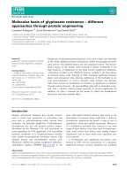
7.2 Scaling of Word Embeddings
Like many NLP systems, the baseline system con-
tains only binary features. The word embeddings,
however, are real numbers that are not necessarily
in a bounded range. If the range of the word
embeddings is too large, they will exert more
influence than the binary features.
We generally found that embeddings had zero
mean. We can scale the embeddings by a hy-
perparameter, to control their standard deviation.

Assume that the embeddings are represented by a
matrix E:
E ← σ · E/stddev(E) (1)
σ is a scaling constant that sets the new standard
deviation after scaling the embeddings.
(a)
93.6
93.8
94
94.2
94.4
94.6
94.8
0.001 0.01 0.1 1
Validation F1
Scaling factor σ
C&W, 50-dim
HLBL, 50-dim
C&W, 200-dim
C&W, 100-dim
HLBL, 100-dim
C&W, 25-dim
baseline
(b)
89
89.5
90
90.5
91
91.5

92
92.5
0.001 0.01 0.1 1
Validation F1
Scaling factor σ
C&W, 200-dim
C&W, 100-dim
C&W, 25-dim
C&W, 50-dim
HLBL, 100-dim
HLBL, 50-dim
baseline
Figure 1: Effect as we vary the scaling factor σ (Equa-
tion 1) on the validation set F1. We experiment with
Collobert and Weston (2008) and HLBL embeddings of var-
ious dimensionality. (a) Chunking results. (b) NER results.
Figure 1 shows the effect of scaling factor σ
on both supervised tasks. We were surprised
to find that on both tasks, across Collobert and
Weston (2008) and HLBL embeddings of various
dimensionality, that all curves had similar shapes
and optima. This is one contributions of our
work. In Turian et al. (2009), we were not
able to prescribe a default value for scaling the
embeddings. However, these curves demonstrate
that a reasonable choice of scale factor is such that
the embeddings have a standard deviation of 0.1.
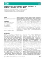
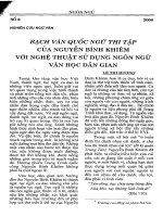
7.3 Capacity of Word Representations
(a)
94.1

94.2
94.3
94.4
94.5
94.6
94.7
100 320 1000 3200
25 50 100 200
Validation F1
# of Brown clusters
# of embedding dimensions
C&W
HLBL
Brown
baseline
(b)
90
90.5
91
91.5
92
92.5
100 320 1000 3200
25 50 100 200
Validation F1
# of Brown clusters
# of embedding dimensions
C&W
Brown
HLBL

baseline
Figure 2: Effect as we vary the capacity of the word
representations on the validation set F1. (a) Chunking
results. (b) NER results.
There are capacity controls for the word
representations: number of Brown clusters, and
number of dimensions of the word embeddings.
Figure 2 shows the effect on the validation F1 as
we vary the capacity of the word representations.
In general, it appears that more Brown clusters
are better. We would like to induce 10000 Brown
clusters, however this would take several months.
In Turian et al. (2009), we hypothesized on
the basis of solely the HLBL NER curve that
higher-dimensional word embeddings would give
higher accuracy. Figure 2 shows that this hy-
pothesis is not true. For NER, the C&W curve is
almost flat, and we were suprised to find the even
25-dimensional C&W word embeddings work so
well. For chunking, 50-dimensional embeddings
had the highest validation F1 for both C&W and
HLBL. These curves indicates that the optimal
capacity of the word embeddings is task-specific.
390
System Dev Test
Baseline 94.16 93.79
HLBL, 50-dim 94.63 94.00
C&W, 50-dim 94.66 94.10
Brown, 3200 clusters 94.67 94.11
Brown+HLBL, 37M 94.62 94.13

C&W+HLBL, 37M 94.68 94.25
Brown+C&W+HLBL, 37M 94.72 94.15
Brown+C&W, 37M 94.76 94.35
Ando and Zhang (2005), 15M - 94.39
Suzuki and Isozaki (2008), 15M - 94.67
Suzuki and Isozaki (2008), 1B - 95.15
Table 2: Final chunking F1 results. In the last section, we
show how many unlabeled words were used.
System Dev Test MUC7
Baseline 90.03 84.39 67.48
Baseline+Nonlocal 91.91 86.52 71.80
HLBL 100-dim 92.00 88.13 75.25
Gazetteers 92.09 87.36 77.76
C&W 50-dim 92.27 87.93 75.74
Brown, 1000 clusters 92.32 88.52 78.84
C&W 200-dim 92.46 87.96 75.51
C&W+HLBL 92.52 88.56 78.64
Brown+HLBL 92.56 88.93 77.85
Brown+C&W 92.79 89.31 80.13
HLBL+Gaz 92.91 89.35 79.29
C&W+Gaz 92.98 88.88 81.44
Brown+Gaz 93.25 89.41 82.71
Lin and Wu (2009), 3.4B - 88.44 -
Ando and Zhang (2005), 27M 93.15 89.31 -
Suzuki and Isozaki (2008), 37M 93.66 89.36 -
Suzuki and Isozaki (2008), 1B 94.48 89.92 -
All (Brown+C&W+HLBL+Gaz), 37M 93.17 90.04 82.50
All+Nonlocal, 37M 93.95 90.36 84.15
Lin and Wu (2009), 700B - 90.90 -
Table 3: Final NER F1 results, showing the cumulative

effect of adding word representations, non-local features, and
gazetteers to the baseline. To speed up training, in combined
experiments (C&W plus another word representation),
we used the 50-dimensional C&W embeddings, not the
200-dimensional ones. In the last section, we show how
many unlabeled words were used.
7.4 Final results
Table 2 shows the final chunking results and Ta-
ble 3 shows the final NER F1 results. We compare
to the state-of-the-art methods of Ando and Zhang
(2005), Suzuki and Isozaki (2008), and—for
NER—Lin and Wu (2009). Tables 2 and 3 show
that accuracy can be increased further by combin-
ing the features from different types of word rep-
resentations. But, if only one word representation
is to be used, Brown clusters have the highest ac-
curacy. Given the improvements to the C&W em-
beddings since Turian et al. (2009), C&W em-
beddings outperform the HLBL embeddings. On
chunking, there is only a minute difference be-
tween Brown clusters and the embeddings. Com-
(a)
0
50
100
150
200
250
0 1 10 100 1K 10K 100K 1M
# of per-token errors (test set)

Frequency of word in unlabeled data
C&W, 50-dim
Brown, 3200 clusters
(b)
0
50
100
150
200
250
0 1 10 100 1K 10K 100K 1M
# of per-token errors (test set)
Frequency of word in unlabeled data
C&W, 50-dim
Brown, 1000 clusters
Figure 3: For word tokens that have different frequency
in the unlabeled data, what is the total number of per-token
errors incurred on the test set? (a) Chunking results. (b) NER
results.
bining representations leads to small increases in
the test F1. In comparison to chunking, combin-
ing different word representations on NER seems
gives larger improvements on the test F1.
On NER, Brown clusters are superior to the
word embeddings. Since much of the NER F1
is derived from decisions made over rare words,
we suspected that Brown clustering has a superior
representation for rare words. Brown makes
a single hard clustering decision, whereas the
embedding for a rare word is close to its initial

value since it hasn’t received many training
updates (see Footnote 2). Figure 3 shows the total
number of per-token errors incurred on the test
set, depending upon the frequency of the word
token in the unlabeled data. For NER, Figure 3 (b)
shows that most errors occur on rare words, and
that Brown clusters do indeed incur fewer errors
for rare words. This supports our hypothesis
that, for rare words, Brown clustering produces
better representations than word embeddings that
haven’t received sufficient training updates. For
chunking, Brown clusters and C&W embeddings
incur almost identical numbers of errors, and
errors are concentrated around the more common
391
words. We hypothesize that non-rare words have
good representations, regardless of the choice
of word representation technique. For tasks like
chunking in which a syntactic decision relies upon
looking at several token simultaneously, com-
pound features that use the word representations
might increase accuracy more (Koo et al., 2008).
Using word representations in NER brought
larger gains on the out-of-domain data than on the
in-domain data. We were surprised by this result,
because the OOD data was not even used during
the unsupervised word representation induction,
as was the in-domain data. We are curious to
investigate this phenomenon further.
Ando and Zhang (2005) present a semi-

supervised learning algorithm called alternating
structure optimization (ASO). They find a low-
dimensional projection of the input features that
gives good linear classifiers over auxiliary tasks.
These auxiliary tasks are sometimes specific
to the supervised task, and sometimes general
language modeling tasks like “predict the missing
word”. Suzuki and Isozaki (2008) present a semi-
supervised extension of CRFs. (In Suzuki et al.
(2009), they extend their semi-supervised ap-
proach to more general conditional models.) One
of the advantages of the semi-supervised learning
approach that we use is that it is simpler and more
general than that of Ando and Zhang (2005) and
Suzuki and Isozaki (2008). Their methods dictate
a particular choice of model and training regime
and could not, for instance, be used with an NLP
system based upon an SVM classifier.
Lin and Wu (2009) present a K-means-like
non-hierarchical clustering algorithm for phrases,
which uses MapReduce. Since they can scale
to millions of phrases, and they train over 800B
unlabeled words, they achieve state-of-the-art
accuracy on NER using their phrase clusters.
This suggests that extending word representa-
tions to phrase representations is worth further
investigation.
8 Conclusions
Word features can be learned in advance in an
unsupervised, task-inspecific, and model-agnostic

manner. These word features, once learned, are
easily disseminated with other researchers, and
easily integrated into existing supervised NLP
systems. The disadvantage, however, is that ac-
curacy might not be as high as a semi-supervised
method that includes task-specific information
and that jointly learns the supervised and unsu-
pervised tasks (Ando & Zhang, 2005; Suzuki &
Isozaki, 2008; Suzuki et al., 2009).
Unsupervised word representations have been
used in previous NLP work, and have demon-
strated improvements in generalization accuracy
on a variety of tasks. Ours is the first work to
systematically compare different word repre-
sentations in a controlled way. We found that
Brown clusters and word embeddings both can
improve the accuracy of a near-state-of-the-art
supervised NLP system. We also found that com-
bining different word representations can improve
accuracy further. Error analysis indicates that
Brown clustering induces better representations
for rare words than C&W embeddings that have
not received many training updates.
Another contribution of our work is a default
method for setting the scaling parameter for
word embeddings. With this contribution, word
embeddings can now be used off-the-shelf as
word features, with no tuning.
Future work should explore methods for
inducing phrase representations, as well as tech-

niques for increasing in accuracy by using word
representations in compound features.
Replicating our experiments
You can visit />projects/wordreprs/ to find: The word
representations we induced, which you can
download and use in your experiments; The code
for inducing the word representations, which you
can use to induce word representations on your
own data; The NER and chunking system, with
code for replicating our experiments.
Acknowledgments
Thank you to Magnus Sahlgren, Bob Carpenter,
Percy Liang, Alexander Yates, and the anonymous
reviewers for useful discussion. Thank you to
Andriy Mnih for inducing his embeddings on
RCV1 for us. Joseph Turian and Yoshua Bengio
acknowledge the following agencies for re-
search funding and computing support: NSERC,
RQCHP, CIFAR. Lev Ratinov was supported by
the Air Force Research Laboratory (AFRL) under
prime contract no. FA8750-09-C-0181. Any
opinions, findings, and conclusion or recommen-
dations expressed in this material are those of the
author and do not necessarily reflect the view of
the Air Force Research Laboratory (AFRL).
392
References
Ando, R., & Zhang, T. (2005). A high-
performance semi-supervised learning method
for text chunking. ACL.

Bengio, Y. (2008). Neural net language models.
Scholarpedia, 3, 3881.
Bengio, Y., Ducharme, R., & Vincent, P. (2001).
A neural probabilistic language model. NIPS.
Bengio, Y., Ducharme, R., Vincent, P., & Jauvin,
C. (2003). A neural probabilistic language
model. Journal of Machine Learning Research,
3, 1137–1155.
Bengio, Y., Louradour, J., Collobert, R., &
Weston, J. (2009). Curriculum learning. ICML.
Bengio, Y., & S
´
en
´
ecal, J S. (2003). Quick train-
ing of probabilistic neural nets by importance
sampling. AISTATS.
Blei, D. M., Ng, A. Y., & Jordan, M. I. (2003).
Latent dirichlet allocation. Journal of Machine
Learning Research, 3, 993–1022.
Brown, P. F., deSouza, P. V., Mercer, R. L., Pietra,
V. J. D., & Lai, J. C. (1992). Class-based n-gram
models of natural language. Computational
Linguistics, 18, 467–479.
Candito, M., & Crabb
´
e, B. (2009). Improving gen-
erative statistical parsing with semi-supervised
word clustering. IWPT (pp. 138–141).
Collobert, R., & Weston, J. (2008). A unified

architecture for natural language processing:
Deep neural networks with multitask learning.
ICML.
Deschacht, K., & Moens, M F. (2009). Semi-
supervised semantic role labeling using the
Latent Words Language Model. EMNLP (pp.
21–29).
Dumais, S. T., Furnas, G. W., Landauer, T. K.,
Deerwester, S., & Harshman, R. (1988). Using
latent semantic analysis to improve access to
textual information. SIGCHI Conference on
Human Factors in Computing Systems (pp.
281–285). ACM.
Elman, J. L. (1993). Learning and development
in neural networks: The importance of starting
small. Cognition, 48, 781–799.
Goldberg, Y., Tsarfaty, R., Adler, M., & Elhadad,
M. (2009). Enhancing unlexicalized parsing
performance using a wide coverage lexicon,
fuzzy tag-set mapping, and EM-HMM-based
lexical probabilities. EACL.
Honkela, T. (1997). Self-organizing maps of
words for natural language processing applica-
tions. Proceedings of the International ICSC
Symposium on Soft Computing.
Honkela, T., Pulkki, V., & Kohonen, T. (1995).
Contextual relations of words in grimm tales,
analyzed by self-organizing map. ICANN.
Huang, F., & Yates, A. (2009). Distributional rep-
resentations for handling sparsity in supervised

sequence labeling. ACL.
Kaski, S. (1998). Dimensionality reduction by
random mapping: Fast similarity computation
for clustering. IJCNN (pp. 413–418).
Koo, T., Carreras, X., & Collins, M. (2008).
Simple semi-supervised dependency parsing.
ACL (pp. 595–603).
Krishnan, V., & Manning, C. D. (2006). An
effective two-stage model for exploiting non-
local dependencies in named entity recognition.
COLING-ACL.
Landauer, T. K., Foltz, P. W., & Laham, D. (1998).
An introduction to latent semantic analysis.
Discourse Processes, 259–284.
Li, W., & McCallum, A. (2005). Semi-supervised
sequence modeling with syntactic topic models.
AAAI.
Liang, P. (2005). Semi-supervised learning
for natural language. Master’s thesis, Mas-
sachusetts Institute of Technology.
Lin, D., & Wu, X. (2009). Phrase clustering
for discriminative learning. ACL-IJCNLP (pp.
1030–1038).
Lund, K., & Burgess, C. (1996). Producing
highdimensional semantic spaces from lexical
co-occurrence. Behavior Research Methods,
Instrumentation, and Computers, 28, 203–208.
Lund, K., Burgess, C., & Atchley, R. A. (1995).
Semantic and associative priming in high-
dimensional semantic space. Cognitive Science

Proceedings, LEA (pp. 660–665).
Martin, S., Liermann, J., & Ney, H. (1998). Algo-
rithms for bigram and trigram word clustering.
Speech Communication, 24, 19–37.
Miller, S., Guinness, J., & Zamanian, A. (2004).
Name tagging with word clusters and discrim-
inative training. HLT-NAACL (pp. 337–342).
393
Mnih, A., & Hinton, G. E. (2007). Three
new graphical models for statistical language
modelling. ICML.
Mnih, A., & Hinton, G. E. (2009). A scalable
hierarchical distributed language model. NIPS
(pp. 1081–1088).
Morin, F., & Bengio, Y. (2005). Hierarchical
probabilistic neural network language model.
AISTATS.
Pereira, F., Tishby, N., & Lee, L. (1993). Distri-
butional clustering of english words. ACL (pp.
183–190).
Ratinov, L., & Roth, D. (2009). Design chal-
lenges and misconceptions in named entity
recognition. CoNLL.
Ritter, H., & Kohonen, T. (1989). Self-organizing
semantic maps. Biological Cybernetics,
241–254.
Sahlgren, M. (2001). Vector-based semantic
analysis: Representing word meanings based
on random labels. Proceedings of the Semantic
Knowledge Acquisition and Categorisation

Workshop, ESSLLI.
Sahlgren, M. (2005). An introduction to random
indexing. Methods and Applications of Seman-
tic Indexing Workshop at the 7th International
Conference on Terminology and Knowledge
Engineering (TKE).
Sahlgren, M. (2006). The word-space model:
Using distributional analysis to represent syn-
tagmatic and paradigmatic relations between
words in high-dimensional vector spaces.
Doctoral dissertation, Stockholm University.
Sang, E. T., & Buchholz, S. (2000). Introduction
to the CoNLL-2000 shared task: Chunking.
CoNLL.
Schwenk, H., & Gauvain, J L. (2002). Connec-
tionist language modeling for large vocabulary
continuous speech recognition. International
Conference on Acoustics, Speech and Signal
Processing (ICASSP) (pp. 765–768). Orlando,
Florida.
Sha, F., & Pereira, F. C. N. (2003). Shal-
low parsing with conditional random fields.
HLT-NAACL.
Spitkovsky, V., Alshawi, H., & Jurafsky, D.
(2010). From baby steps to leapfrog: How “less
is more” in unsupervised dependency parsing.
NAACL-HLT.
Suzuki, J., & Isozaki, H. (2008). Semi-supervised
sequential labeling and segmentation using
giga-word scale unlabeled data. ACL-08: HLT

(pp. 665–673).
Suzuki, J., Isozaki, H., Carreras, X., & Collins, M.
(2009). An empirical study of semi-supervised
structured conditional models for dependency
parsing. EMNLP.
Turian, J., Ratinov, L., Bengio, Y., & Roth, D.
(2009). A preliminary evaluation of word
representations for named-entity recognition.
NIPS Workshop on Grammar Induction, Repre-
sentation of Language and Language Learning.
Turney, P. D., & Pantel, P. (2010). From frequency
to meaning: Vector space models of semantics.
Journal of Artificial Intelligence Research.
Ushioda, A. (1996). Hierarchical clustering of
words. COLING (pp. 1159–1162).
V
¨
ayrynen, J., & Honkela, T. (2005). Compar-
ison of independent component analysis and
singular value decomposition in word context
analysis. AKRR’05, International and Interdis-
ciplinary Conference on Adaptive Knowledge
Representation and Reasoning.
V
¨
ayrynen, J. J., & Honkela, T. (2004). Word cat-
egory maps based on emergent features created
by ICA. Proceedings of the STeP’2004 Cogni-
tion + Cybernetics Symposium (pp. 173–185).
Finnish Artificial Intelligence Society.

V
¨
ayrynen, J. J., Honkela, T., & Lindqvist, L.
(2007). Towards explicit semantic features
using independent component analysis. Pro-
ceedings of the Workshop Semantic Content
Acquisition and Representation (SCAR). Stock-
holm, Sweden: Swedish Institute of Computer
Science.
ˇ
Reh
˚
u
ˇ
rek, R., & Sojka, P. (2010). Software frame-
work for topic modelling with large corpora.
LREC.
Zhang, T., & Johnson, D. (2003). A robust risk
minimization based named entity recognition
system. CoNLL.
Zhao, H., Chen, W., Kit, C., & Zhou, G.
(2009). Multilingual dependency learning: a
huge feature engineering method to semantic
dependency parsing. CoNLL (pp. 55–60).
394