Tài liệu Báo cáo khoa học: "Learning Sub-Word Units for Open Vocabulary Speech Recognition" doc

Proceedings of the 49th Annual Meeting of the Association for Computational Linguistics, pages 712–721,
Portland, Oregon, June 19-24, 2011.
c
2011 Association for Computational Linguistics
Learning Sub-Word Units for Open Vocabulary Speech Recognition
Carolina Parada
1
, Mark Dredze
1
, Abhinav Sethy
2
, and Ariya Rastrow
1
1
Human Language Technology Center of Excellence, Johns Hopkins University
3400 N Charles Street, Baltimore, MD, USA
, ,
2
IBM T.J. Watson Research Center, Yorktown Heights, NY, USA

Abstract
Large vocabulary speech recognition systems
fail to recognize words beyond their vocab-
ulary, many of which are information rich
terms, like named entities or foreign words.
Hybrid word/sub-word systems solve this
problem by adding sub-word units to large vo-
cabulary word based systems; new words can
then be represented by combinations of sub-
word units. Previous work heuristically cre-
ated the sub-word lexicon from phonetic rep-

resentations of text using simple statistics to
select common phone sequences. We pro-
pose a probabilistic model to learn the sub-
word lexicon optimized for a given task. We
consider the task of out of vocabulary (OOV)
word detection, which relies on output from
a hybrid model. A hybrid model with our
learned sub-word lexicon reduces error by
6.3% and 7.6% (absolute) at a 5% false alarm
rate on an English Broadcast News and MIT
Lectures task respectively.
1 Introduction
Most automatic speech recognition systems operate
with a large but limited vocabulary, finding the most
likely words in the vocabulary for the given acoustic
signal. While large vocabulary continuous speech
recognition (LVCSR) systems produce high quality
transcripts, they fail to recognize out of vocabulary
(OOV) words. Unfortunately, OOVs are often infor-
mation rich nouns, such as named entities and for-
eign words, and mis-recognizing them can have a
disproportionate impact on transcript coherence.
Hybrid word/sub-word recognizers can produce a
sequence of sub-word units in place of OOV words.
Ideally, the recognizer outputs a complete word for
in-vocabulary (IV) utterances, and sub-word units
for OOVs. Consider the word “Slobodan”, the given
name of the former president of Serbia. As an un-
common English word, it is unlikely to be in the vo-
cabulary of an English recognizer. While a LVCSR

system would output the closest known words (e.x.
“slow it dawn”), a hybrid system could output a
sequence of multi-phoneme units: s l ow, b ax,
d ae n. The latter is more useful for automatically
recovering the word’s orthographic form, identify-
ing that an OOV was spoken, or improving perfor-
mance of a spoken term detection system with OOV
queries. In fact, hybrid systems have improved OOV
spoken term detection (Mamou et al., 2007; Parada
et al., 2009), achieved better phone error rates, espe-
cially in OOV regions (Rastrow et al., 2009b), and
obtained state-of-the-art performance for OOV de-
tection (Parada et al., 2010).
Hybrid recognizers vary in a number of ways:
sub-word unit type: variable-length phoneme
units (Rastrow et al., 2009a; Bazzi and Glass, 2001)
or joint letter sound sub-words (Bisani and Ney,
2005); unit creation: data-driven or linguistically
motivated (Choueiter, 2009); and how they are in-
corporated in LVCSR systems: hierarchical (Bazzi,
2002) or flat models (Bisani and Ney, 2005).
In this work, we consider how to optimally cre-
ate sub-word units for a hybrid system. These units
are variable-length phoneme sequences, although in
principle our work can be use for other unit types.
Previous methods for creating the sub-word lexi-
712
con have relied on simple statistics computed from
the phonetic representation of text (Rastrow et al.,
2009a). These units typically represent the most fre-

quent phoneme sequences in English words. How-
ever, it isn’t clear why these units would produce the
best hybrid output. Instead, we introduce a prob-
abilistic model for learning the optimal units for a
given task. Our model learns a segmentation of a
text corpus given some side information: a mapping
between the vocabulary and a label set; learned units
are predictive of class labels.
In this paper, we learn sub-word units optimized
for OOV detection. OOV detection aims to identify
regions in the LVCSR output where OOVs were ut-
tered. Towards this goal, we are interested in select-
ing units such that the recognizer outputs them only
for OOV regions while prefering to output a com-
plete word for in-vocabulary regions. Our approach
yields improvements over state-of-the-art results.
We begin by presenting our log-linear model for
learning sub-word units with a simple but effective
inference procedure. After reviewing existing OOV
detection approaches, we detail how the learned
units are integrated into a hybrid speech recognition
system. We show improvements in OOV detection,
and evaluate impact on phone error rates.
2 Learning Sub-Word Units
Given raw text, our objective is to produce a lexicon
of sub-word units that can be used by a hybrid sys-
tem for open vocabulary speech recognition. Rather
than relying on the text alone, we also utilize side
information: a mapping of words to classes so we
can optimize learning for a specific task.

The provided mapping assigns labels Y to the cor-
pus. We maximize the probability of the observed
labeling sequence Y given the text W : P (Y |W ).
We assume there is a latent segmentation S of this
corpus which impacts Y . The complete data likeli-
hood becomes: P (Y |W ) =

S
P (Y, S|W ) during
training. Since we are maximizing the observed Y ,
segmentation S must discriminate between different
possible labels.
We learn variable-length multi-phone units by
segmenting the phonetic representation of each word
in the corpus. Resulting segments form the sub-
word lexicon.
1
Learning input includes a list of
words to segment taken from raw text, a mapping
between words and classes (side information indi-
cating whether token is IV or OOV), a pronuncia-
tion dictionary D, and a letter to sound model (L2S),
such as the one described in Chen (2003). The cor-
pus W is the list of types (unique words) in the raw
text input. This forces each word to have a unique
segmentation, shared by all common tokens. Words
are converted into phonetic representations accord-
ing to their most likely dictionary pronunciation;
non-dictionary words use the L2S model.
2

2.1 Model
Inspired by the morphological segmentation model
of Poon et al. (2009), we assume P (Y, S|W ) is a
log-linear model parameterized by Λ:
P
Λ
(Y, S|W ) =
1
Z(W )
u
Λ
(Y, S, W ) (1)
where u
Λ
(Y, S, W ) defines the score of the pro-
posed segmentation S for words W and labels Y
according to model parameters Λ. Sub-word units
σ compose S, where each σ is a phone sequence, in-
cluding the full pronunciation for vocabulary words;
the collection of σs form the lexicon. Each unit
σ is present in a segmentation with some context
c = (φ
l
, φ
r
) of the form φ
l
σφ
r
. Features based on

the context and the unit itself parameterize u
Λ
.
In addition to scoring a segmentation based on
features, we include two priors inspired by the Min-
imum Description Length (MDL) principle sug-
gested by Poon et al. (2009). The lexicon prior
favors smaller lexicons by placing an exponential
prior with negative weight on the length of the lex-
icon

σ
|σ|, where |σ| is the length of the unit σ
in number of phones. Minimizing the lexicon prior
favors a trivial lexicon of only the phones. The
corpus prior counters this effect, an exponential
prior with negative weight on the number of units
in each word’s segmentation, where |s
i
| is the seg-
mentation length and |w
i
| is the length of the word
in phones. Learning strikes a balance between the
two priors. Using these definitions, the segmenta-
tion score u
Λ
(Y, S, W ) is given as:
1
Since sub-word units can expand full-words, we refer to

both words and sub-words simply as units.
2
The model can also take multiple pronunciations (§3.1).
713
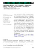
s l ow b ax d ae n
s l ow
(#,#, , b, ax)
b ax
(l,ow, , d, ae)
d ae n
(b,ax, , #, #)
Figure 1: Units and bigram phone context (in parenthesis)
for an example segmentation of the word “slobodan”.
u
Λ
(Y, S, W ) = exp


σ,y
λ
σ,y
f
σ,y
(S, Y )
+

c,y
λ
c,y
f

c,y
(S, Y )
+ α ·

σ∈S
|σ|
+ β ·

i∈W
|s
i
|/|w
i
|

(2)
f
σ,y
(S, Y ) are the co-occurrence counts of the pair
(σ, y) where σ is a unit under segmentation S and y
is the label. f
c,y
(S, Y ) are the co-occurrence counts
for the context c and label y under S. The model
parameters are Λ = {λ
σ,y
, λ
c,y
: ∀σ, c, y}. The neg-
ative weights for the lexicon (α) and corpus priors

(β) are tuned on development data. The normalizer
Z sums over all possible segmentations and labels:
Z(W ) =

S


Y

u
Λ
(Y

, S

, W ) (3)
Consider the example segmentation for the word
“slobodan” with pronunciation s,l,ow,b,ax,d,ae,n
(Figure 1). The bigram phone context as a four-tuple
appears below each unit; the first two entries corre-
spond to the left context, and last two the right con-
text. The example corpus (Figure 2) demonstrates
how unit features f
σ,y
and context features f
c,y
are
computed.
3 Model Training
Learning maximizes the log likelihood of the ob-

served labels Y
∗
given the words W :
(Y
∗
|W ) = log

S
1
Z(W )
u
Λ
(Y
∗
, S, W ) (4)
We use the Expectation-Maximization algorithm,
where the expectation step predicts segmentations S
Labeled corpus: president/y = 0 milosevic/y = 1
Segmented corpus: p r eh z ih d ih n t/0 m ih/1 l aa/1
s ax/1 v ih ch/1
Unit-feature:Value p r eh z ih d ih n t/0:1 m ih/1:1
l aa/1:1 s ax/1:1 v ih ch/1:1
Context-feature:Value
(#/0,#/0, ,l/1,aa/1):1,
(m/1,ih/1, ,s/1,ax/1):1,
(l/1,aa/1, ,v/1,ih/1):1,
(s/1,ax/1, ,#/0,#/0):1,
(#/0,#/0, ,#/0,#/0):1
Figure 2: A small example corpus with segmentations
and corresponding features. The notation m ih/1:1

represents unit/label:feature-value. Overlapping context
features capture rich segmentation regularities associated
with each class.
given the model’s current parameters Λ (§3.1), and
the maximization step updates these parameters us-
ing gradient ascent. The partial derivatives of the
objective (4) with respect to each parameter λ
i
are:
∂(Y
∗
|W )
∂λ
i
= E
S|Y
∗
,W
[f
i
] − E
S,Y |W
[f
i
] (5)
The gradient takes the usual form, where we en-
courage the expected segmentation from the current
model given the correct labels to equal the expected
segmentation and expected labels. The next section
discusses computing these expectations.

3.1 Inference
Inference is challenging since the lexicon prior ren-
ders all word segmentations interdependent. Con-
sider a simple two word corpus: cesar (s,iy,z,er),
and cesium (s,iy,z,iy,ax,m). Numerous segmen-
tations are possible; each word has 2
N−1
possible
segmentations, where N is the number of phones in
its pronunciation (i.e., 2
3
× 2
5
= 256). However,
if we decide to segment the first word as: {s iy,
z er}, then the segmentation for “cesium”:{s iy,
z iy ax m} will incur a lexicon prior penalty for
including the new segment z iy ax m. If instead
we segment “cesar” as {s iy z, er}, the segmen-
tation {s iy, z iy ax m} incurs double penalty
for the lexicon prior (since we are including two new
units in the lexicon: s iy and z iy ax m). This
dependency requires joint segmentation of the entire
corpus, which is intractable. Hence, we resort to ap-
proximations of the expectations in Eq. (5).
One approach is to use Gibbs Sampling: it-
erating through each word, sampling a new seg-
714
mentation conditioned on the segmentation of all
other words. The sampling distribution requires

enumerating all possible segmentations for each
word (2
N−1
) and computing the conditional prob-
abilities for each segmentation: P (S|Y
∗
, W ) =
P (Y
∗
, S|W )/P(Y
∗
|W ) (the features are extracted
from the remaining words in the corpus). Using M
sampled segmentations S
1
, S
2
, . . . S
m
we compute
E
S|Y
∗
,W
[f
i
] as follows:
E
S|Y
∗

,W
[f
i
] ≈
1
M

j
f
i
[S
j
]
Similarly, to compute E
S,Y |W
we sample a seg-
mentation and a label for each word. We com-
pute the joint probability of P (Y, S|W ) for each
segmentation-label pair using Eq. (1). A sampled
segmentation can introduce new units, which may
have higher probability than existing ones.
Using these approximations in Eq. (5), we update
the parameters using gradient ascent:
¯
λ
new
=
¯
λ
old

+ γ∇
¯
λ
(Y
∗
|W )
where γ > 0 is the learning rate.
To obtain the best segmentation, we use determin-
istic annealing. Sampling operates as usual, except
that the parameters are divided by a value, which
starts large and gradually drops to zero. To make
burn in faster for sampling, the sampler is initialized
with the most likely segmentation from the previous
iteration. To initialize the sampler the first time, we
set all the parameters to zero (only the priors have
non-zero values) and run deterministic annealing to
obtain the first segmentation of the corpus.
3.2 Efficient Sampling
Sampling a segmentation for the corpus requires
computing the normalization constant (3), which
contains a summation over all possible corpus seg-
mentations. Instead, we approximate this constant
by sampling words independently, keeping fixed all
other segmentations. Still, even sampling a single
word’s segmentation requires enumerating probabil-
ities for all possible segmentations.
We sample a segmentation efficiently using dy-
namic programming. We can represent all possible
segmentations for a word as a finite state machine
(FSM) (Figure 3), where arcs weights arise from

scoring the segmentation’s features. This weight is
the negative log probability of the resulting model
after adding the corresponding features and priors.
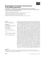
However, the lexicon prior poses a problem for
this construction since the penalty incurred by a new
unit in the segmentation depends on whether that
unit is present elsewhere in that segmentation. For
example, consider the segmentation for the word
ANJANI: AA
N, JH, AA N, IY. If none of these units
are in the lexicon, this segmentation yields the low-
est prior penalty since it repeats the unit AA N.
3
This
global dependency means paths must encode the full
unit history, making computing forward-backward
probabilities inefficient.
Our solution is to use the Metropolis-Hastings al-
gorithm, which samples from the true distribution
P (Y, S|W ) by first sampling a new label and seg-
mentation (y

, s

) from a simpler proposal distribu-
tion Q(Y, S|W ). The new assignment (y

, s

) is ac-

cepted with probability:
α(Y

, S

|Y, S, W)=min
„
1,
P (Y

, S

|W )Q(Y, S|Y

, S

, W )
P (Y, S|W )Q(Y

, S

|Y, S, W)
«
We choose the proposal distribution Q(Y, S|W )
as Eq. (1) omitting the lexicon prior, removing the
challenge for efficient computation. The probability
of accepting a sample becomes:
α(Y

, S


|Y, S, W)=min
„
1,
P
σ∈S

|σ|
P
σ∈S
|σ|
«
(6)
We sample a path from the FSM by running the
forward-backward algorithm, where the backward
computations are carried out explicitly, and the for-
ward pass is done through sampling, i.e. we traverse
the machine only computing forward probabilities
for arcs leaving the sampled state.
4
Once we sample
a segmentation (and label) we accept it according to
Eq. (6) or keep the previous segmentation if rejected.
Alg. 1 shows our full sub-word learning proce-
dure, where sampleSL (Alg. 2) samples a segmen-
tation and label sequence for the entire corpus from
P (Y, S|W ), and sampleS samples a segmentation
from P (S|Y
∗
, W ).

3
Splitting at phone boundaries yields the same lexicon prior
but a higher corpus prior.
4
We use OpenFst’s RandGen operation with a costumed arc-
selector ( />715
0 1
AA
5
AA_N_JH_AA_N
4
AA_N_JH_AA
3
AA_N_JH
2
AA_N
N_JH_AA_N
N_JH_AA
N_JH
N
6
N_JH_AA_N_IY
IY
N
AA_N
AA
AA_N_IY
JH_AA_N
JH_AA
JH

JH_AA_N_IY
Figure 3: FSM representing all segmentations for the word ANJANI with pronunciation: AA,N,JH,AA,N,IY
Algorithm 1 Training
Input: Lexicon L from training text W , Dictionary D,
Mapping M, L2S pronunciations, Annealing temp T .
Initialization:
Assign label y
∗
m
= M[w
m
].
¯
λ
0
=
¯
0
S
0
= random segmentation for each word in L.
for i = 1 to K do
/* E-Step */
S
i
= bestSegmentation(T, λ
i−1
, S
i−1
).

for k = 1 to NumSamples do
(S

k
, Y

k
) = sampleSL(P (Y, S
i
|W ),Q(Y, S
i
|W ))
˜
S
k
= sampleS(P (S
i
|Y
∗
, W ),Q(S
i
|Y
∗
, W ))
end for
/* M-Step */
E
S,Y |W
[f
i

] =
1
NumSamples

k
f
σ,l
[S

k
, Y

k
]
E
S|Y
∗
,W
[f
σ,l
] =
1
NumSamples

k
f
σ,l
[
˜
S

k
, Y
∗
]
¯
λ
i
=
¯
λ
i−1
+ γ∇L
¯
λ
(Y
∗
|W )
end for
S = bestSegmentation(T, λ
K
, S
0
)
Output: Lexicon L
o
from S
4 OOV Detection Using Hybrid Models
To evaluate our model for learning sub-word units,
we consider the task of out-of-vocabulary (OOV)
word detection. OOV detection for ASR output can

be categorized into two broad groups: 1) hybrid
(filler) models: which explicitly model OOVs us-
ing either filler, sub-words, or generic word mod-
els (Bazzi, 2002; Schaaf, 2001; Bisani and Ney,
2005; Klakow et al., 1999; Wang, 2009); and
2) confidence-based approaches: which label un-
reliable regions as OOVs based on different con-
fidence scores, such as acoustic scores, language
models, and lattice scores (Lin et al., 2007; Burget
et al., 2008; Sun et al., 2001; Wessel et al., 2001).
In the next section we detail the OOV detection
approach we employ, which combines hybrid and
Algorithm 2 sampleSL(P (S, Y |W ), Q(S, Y |W ))
for m = 1 to M (NumWords) do
(s

m
, y

m
) = Sample segmentation/label pair for
word w
m
according to Q(S, Y |W )
Y

= {y
1
. . . y
m−1

y

m
y
m+1
. . . y
M
}
S

= {s
1
. . . s
m−1
s

m
s
m+1
. . . s
M
}
α=min

1,
P
σ∈S

|σ|
P

σ∈S
|σ|

with prob α : y
m,k
= y

m
, s
m,k
= s

m
with prob (1 − α) : y
m,k
= y
m
, s
m,k
= s
m
end for
return (S

k
, Y

k
) = [(s
1,k

, y
1,k
) . . . (s
M,k
, y
M,k
)]
confidence-based models, achieving state-of-the art
performance for this task.
4.1 OOV Detection Approach
We use the state-of-the-art OOV detection model of
Parada et al. (2010), a second order CRF with fea-
tures based on the output of a hybrid recognizer.
This detector processes hybrid recognizer output, so
we can evaluate different sub-word unit lexicons for
the hybrid recognizer and measure the change in
OOV detection accuracy.
Our model (§2.1) can be applied to this task by
using a dictionary D to label words as IV (y
i
= 0 if
w
i
∈ D) and OOV (y
i
= 1 if w
i
/∈ D). This results
in a labeled corpus, where the labeling sequence Y
indicates the presence of out-of-vocabulary words

(OOVs). For comparison we evaluate a baseline
method (Rastrow et al., 2009b) for selecting units.
Given a sub-word lexicon, the word and sub-
words are combined to form a hybrid language
model (LM) to be used by the LVCSR system. This
hybrid LM captures dependencies between word and
sub-words. In the LM training data, all OOVs are
represented by the smallest number of sub-words
which corresponds to their pronunciation. Pronun-
ciations for all OOVs are obtained using grapheme
716
to phone models (Chen, 2003).
Since sub-words represent OOVs while building
the hybrid LM, the existence of sub-words in ASR
output indicate an OOV region. A simple solution to
the OOV detection problem would then be reduced
to a search for the sub-words in the output of the
ASR system. The search can be on the one-best
transcripts, lattices or confusion networks. While
lattices contain more information, they are harder
to process; confusion networks offer a trade-off be-
tween richness (posterior probabilities are already
computed) and compactness (Mangu et al., 1999).
Two effective indications of OOVs are the exis-
tence of sub-words (Eq. 7) and high entropy in a
network region (Eq. 8), both of which are used as
features in the model of Parada et al. (2010).
Sub-word Posterior =

σ∈t

j
p(σ|t
j
) (7)
Word-Entropy = −

w∈t
j
p(w|t
j
) log p(w|t
j
) (8)
t
j
is the current bin in the confusion network and
σ is a sub-word in the hybrid dictionary. Improving
the sub-word unit lexicon, improves the quality of
the confusion networks for OOV detection.
5 Experimental Setup
We used the data set constructed by Can et al.
(2009) (OOVCORP) for the evaluation of Spoken
Term Detection of OOVs since it focuses on the
OOV problem. The corpus contains 100 hours of
transcribed Broadcast News English speech. There
are 1290 unique OOVs in the corpus, which were
selected with a minimum of 5 acoustic instances per
word and short OOVs inappropriate for STD (less
than 4 phones) were explicitly excluded. Example
OOVs include: NATALIE, PUTIN, QAEDA,

HOLLOWAY, COROLLARIES, HYPERLINKED,
etc. This resulted in roughly 24K (2%) OOV tokens.
For LVCSR, we used the IBM Speech Recogni-
tion Toolkit (Soltau et al., 2005)
5
to obtain a tran-
script of the audio. Acoustic models were trained
on 300 hours of HUB4 data (Fiscus et al., 1998)
and utterances containing OOV words as marked in
OOVCORP were excluded. The language model was
trained on 400M words from various text sources
5
The IBM system used speaker adaptive training based on
maximum likelihood with no discriminative training.
with a 83K word vocabulary. The LVCSR system’s
WER on the standard RT04 BN test set was 19.4%.
Excluded utterances amount to 100hrs. These were
divided into 5 hours of training for the OOV detec-
tor and 95 hours of test. Note that the OOV detector
training set is different from the LVCSR training set.
We also use a hybrid LVCSR system, combin-
ing word and sub-word units obtained from ei-
ther our approach or a state-of-the-art baseline ap-
proach (Rastrow et al., 2009a) (§5.2). Our hybrid
system’s lexicon has 83K words and 5K or 10K
sub-words. Note that the word vocabulary is com-
mon to both systems and only the sub-words are se-
lected using either approach. The word vocabulary
used is close to most modern LVCSR system vo-
cabularies for English Broadcast News; the result-

ing OOVs are more challenging but more realistic
(i.e. mostly named entities and technical terms). The
1290 words are OOVs to both the word and hybrid
systems.
In addition we report OOV detection results on a
MIT lectures data set (Glass et al., 2010) consisting
of 3 Hrs from two speakers with a 1.5% OOV rate.
These were divided into 1 Hr for training the OOV
detector and 2 Hrs for testing. Note that the LVCSR
system is trained on Broadcast News data. This out-
of-domain test-set help us evaluate the cross-domain
performance of the proposed and baseline hybrid
systems. OOVs in this data set correspond mainly to
technical terms in computer science and math. e.g.
ALGORITHM, DEBUG, COMPILER, LISP.
5.1 Learning parameters
For learning the sub-words we randomly selected
from training 5,000 words which belong to the 83K
vocabulary and 5,000 OOVs
6
. For development we
selected an additional 1,000 IV and 1,000 OOVs.
This was used to tune our model hyper parameters
(set to α = −1, β = −20). There is no overlap
of OOVs in training, development and test sets. All
feature weights were initialized to zero and had a
Gaussian prior with variance σ = 100. Each of the
words in training and development was converted to
their most-likely pronunciation using the dictionary
6

This was used to obtain the 5K hybrid system. To learn sub-
words for the 10K hybrid system we used 10K in-vocabulary
words and 10K OOVs. All words were randomly selected from
the LM training text.
717
for IV words or the L2S model for OOVs.
7
The learning rate was γ
k
=
γ
(k+1+A)
τ
, where k is
the iteration, A is the stability constant (set to 0.1K),
γ = 0.4, and τ = 0.6. We used K = 40 itera-
tions for learning and 200 samples to compute the
expectations in Eq. 5. The sampler was initialized
by sampling for 500 iterations with deterministic an-
nealing for a temperature varying from 10 to 0 at 0.1
intervals. Final segmentations were obtained using
10, 000 samples and the same temperature schedule.
We limit segmentations to those including units of at
most 5 phones to speed sampling with no significant
degradation in performance. We observed improved
performance by dis-allowing whole word units.
5.2 Baseline Unit Selection
We used Rastrow et al. (2009a) as our baseline
unit selection method, a data driven approach where
the language model training text is converted into

phones using the dictionary (or a letter-to-sound
model for OOVs), and a N-gram phone LM is es-
timated on this data and pruned using a relative en-
tropy based method. The hybrid lexicon includes
resulting sub-words – ranging from unigrams to 5-
gram phones, and the 83K word lexicon.
5.3 Evaluation
We obtain confusion networks from both the word
and hybrid LVCSR systems. We align the LVCSR
transcripts with the reference transcripts and tag
each confusion region as either IV or OOV. The
OOV detector classifies each region in the confusion
network as IV/OOV. We report OOV detection accu-
racy using standard detection error tradeoff (DET)
curves (Martin et al., 1997). DET curves measure
tradeoffs between false alarms (x-axis) and misses
(y-axis), and are useful for determining the optimal
operating point for an application; lower curves are
better. Following Parada et al. (2010) we separately
evaluate unobserved OOVs.
8
7
In this work we ignore pronunciation variability and sim-
ply consider the most likely pronunciation for each word. It
is straightforward to extend to multiple pronunciations by first
sampling a pronunciation for each word and then sampling a
segmentation for that pronunciation.
8
Once an OOV word has been observed in the OOV detector
training data, even if it was not in the LVCSR training data, it is

no longer truly OOV.
6 Results
We compare the performance of a hybrid sys-
tem with baseline units
9
(§5.2) and one with units
learned by our model on OOV detection and phone
error rate. We present results using a hybrid system
with 5k and 10k sub-words.
We evaluate the CRF OOV detector with two dif-
ferent feature sets. The first uses only Word En-
tropy and Sub-word Posterior (Eqs. 7 and 8) (Fig-
ure 4)
10
. The second (context) uses the extended
context features of Parada et al. (2010) (Figure 5).
Specifically, we include all trigrams obtained from
the best hypothesis of the recognizer (a window of 5
words around current confusion bin). Predictions at
different FA rates are obtained by varying a proba-
bility threshold.
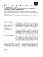
At a 5% FA rate, our system (This Paper 5k) re-
duces the miss OOV rate by 6.3% absolute over the
baseline (Baseline 5k) when evaluating all OOVs.
For unobserved OOVs, it achieves 3.6% absolute
improvement. A larger lexicon (Baseline 10k and
This Paper 10k ) shows similar relative improve-
ments. Note that the features used so far do not nec-
essarily provide an advantage for unobserved ver-
sus observed OOVs, since they ignore the decoded

word/sub-word sequence. In fact, the performance
on un-observed OOVs is better.
OOV detection improvements can be attributed to
increased coverage of OOV regions by the learned
sub-words compared to the baseline. Table 1 shows
the percent of Hits: sub-word units predicted in
OOV regions, and False Alarms: sub-word units
predicted for in-vocabulary words. We can see
that the proposed system increases the Hits by over
8% absolute, while increasing the False Alarms by
0.3%. Interestingly, the average sub-word length
for the proposed units exceeded that of the baseline
units by 0.3 phones (Baseline 5K average length
was 2.92, while that of This Paper 5K was 3.2).
9
Our baseline results differ from Parada et al. (2010). When
implementing the lexicon baseline, we discovered that their hy-
brid units were mistakenly derived from text containing test
OOVs. Once excluded, the relative improvements of previous
work remain, but the absolute error rates are higher.
10
All real-valued features were normalized and quantized us-
ing the uniform-occupancy partitioning described in White et
al. (2007). We used 50 partitions with a minimum of 100 train-
ing values per partition.
718
(a) (b)
Figure 4: DET curves for OOV detection using baseline hybrid systems for different lexicon size and proposed dis-
criminative hybrid system on OOVCORP data set. Evaluation on un-observed OOVs (a) and all OOVs (b).
(a) (b)

Figure 5: Effect of adding context features to baseline and discriminative hybrid systems on OOVCORP data set.
Evaluation on un-observed OOVs (a) and all OOVs (b).
Consistent with previously published results, in-
cluding context achieves large improvement in per-
formance. The proposed hybrid system (This Pa-
per 10k + context-features) still improves over the
baseline (Baseline 10k + context-features), however
the relative gain is reduced. In this case, we ob-
tain larger gains for un-observed OOVs which ben-
efit less from the context clues learned in training.
Lastly, we report OOV detection performance on
MIT Lectures. Both the sub-word lexicon and the
LVCSR models were trained on Broadcast News
data, helping us evaluate the robustness of learned
sub-words across domains. Note that the OOVs
in these domains are quite different: MIT Lec-
tures’ OOVs correspond to technical computer sci-
Hybrid System Hits FAs
Baseline (5k) 18.25 1.49
This Paper (5k) 26.78 1.78
Baseline (10k) 24.26 1.82
This Paper (10k) 28.96 1.92
Table 1: Coverage of OOV regions by baseline and pro-
posed sub-words in OOVCORP.
ence and math terms, while in Broadcast News they
are mainly named-entities.
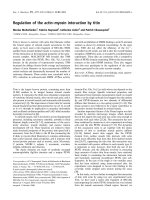
Figure 6 and 7 show the OOV detection results in
the MIT Lectures data set. For un-observed OOVs,
the proposed system (This Paper 10k) reduces the
miss OOV rate by 7.6% with respect to the base-

line (Baseline 10k) at a 5% FA rate. Similar to
Broadcast News results, we found that the learned
sub-words provide larger coverage of OOV regions
in MIT Lectures domain. These results suggest that
the proposed sub-words are not simply modeling the
training OOVs (named-entities) better than the base-
line sub-words, but also describe better novel unex-
pected words. Furthermore, including context fea-
tures does not seem as helpful. We conjecture that
this is due to the higher WER
11
and the less struc-
tured nature of the domain: i.e. ungrammatical sen-
tences, disfluencies, incomplete sentences, making
it more difficult to predict OOVs based on context.
11
W ER = 32.7% since the LVCSR system was trained on
Broadcast News data as described in Section 5.
719
(a) (b)
Figure 6: DET curves for OOV detection using baseline hybrid systems for different lexicon size and proposed dis-
criminative hybrid system on MIT Lectures data set. Evaluation on un-observed OOVs (a) and all OOVs (b).
(a) (b)
Figure 7: Effect of adding context features to baseline and discriminative hybrid systems on MIT Lectures data set.
Evaluation on un-observed OOVs (a) and all OOVs (b).
6.1 Improved Phonetic Transcription
We consider the hybrid lexicon’s impact on Phone
Error Rate (PER) with respect to the reference tran-
scription. The reference phone sequence is obtained
by doing forced alignment of the audio stream to the

reference transcripts using acoustic models. This
provides an alignment of the pronunciation variant
of each word in the reference and the recognizer’s
one-best output. The aligned words are converted to
the phonetic representation using the dictionary.
Table 2 presents PERs for the word and differ-
ent hybrid systems. As previously reported (Ras-
trow et al., 2009b), the hybrid systems achieve bet-
ter PER, specially in OOV regions since they pre-
dict sub-word units for OOVs. Our method achieves
modest improvements in PER compared to the hy-
brid baseline. No statistically significant improve-
ments in PER were observed on MIT Lectures.
7 Conclusions
Our probabilistic model learns sub-word units for
hybrid speech recognizers by segmenting a text cor-
pus while exploiting side information. Applying our
System OOV IV All
Word 1.62 6.42 8.04
Hybrid: Baseline (5k) 1.56 6.44 8.01
Hybrid: Baseline (10k) 1.51 6.41 7.92
Hybrid: This Paper (5k) 1.52 6.42 7.94
Hybrid: This Paper (10k) 1.45 6.39 7.85
Table 2: Phone Error Rate for OOVCORP.
method to the task of OOV detection, we obtain an
absolute error reduction of 6.3% and 7.6% at a 5%
false alarm rate on an English Broadcast News and
MIT Lectures task respectively, when compared to a
baseline system. Furthermore, we have confirmed
previous work that hybrid systems achieve better

phone accuracy, and our model makes modest im-
provements over a baseline with a similarly sized
sub-word lexicon. We plan to further explore our
new lexicon’s performance for other languages and
tasks, such as OOV spoken term detection.
Acknowledgments
We gratefully acknowledge Bhuvaha Ramabhadran
for many insightful discussions and the anonymous
reviewers for their helpful comments. This work
was funded by a Google PhD Fellowship.
720
References
Issam Bazzi and James Glass. 2001. Learning units
for domain-independent out-of-vocabulary word mod-
eling. In EuroSpeech.
Issam Bazzi. 2002. Modelling out-of-vocabulary words
for robust speech recognition. Ph.D. thesis, Mas-
sachusetts Institute of Technology.
M. Bisani and H. Ney. 2005. Open vocabulary speech
recognition with flat hybrid models. In INTER-
SPEECH.
L. Burget, P. Schwarz, P. Matejka, M. Hannemann,
A. Rastrow, C. White, S. Khudanpur, H. Hermansky,
and J. Cernocky. 2008. Combination of strongly and
weakly constrained recognizers for reliable detection
of OOVS. In ICASSP.
D. Can, E. Cooper, A. Sethy, M. Saraclar, and C. White.
2009. Effect of pronounciations on OOV queries in
spoken term detection. Proceedings of ICASSP.
Stanley F. Chen. 2003. Conditional and joint models

for grapheme-to-phoneme conversion. In Eurospeech,
pages 2033–2036.
G. Choueiter. 2009. Linguistically-motivated sub-
word modeling with applications to speech recogni-
tion. Ph.D. thesis, Massachusetts Institute of Technol-
ogy.
Jonathan Fiscus, John Garofolo, Mark Przybocki,
William Fisher, and David Pallett, 1998. 1997 En-
glish Broadcast News Speech (HUB4). Linguistic
Data Consortium, Philadelphia.
James Glass, Timothy Hazen, Lee Hetherington, and
Chao Wang. 2010. Analysis and processing of lec-
ture audio data: Preliminary investigations. In North
American Chapter of the Association for Computa-
tional Linguistics (NAACL).
Dietrich Klakow, Georg Rose, and Xavier Aubert. 1999.
OOV-detection in large vocabulary system using au-
tomatically defined word-fragments as fillers. In Eu-
rospeech.
Hui Lin, J. Bilmes, D. Vergyri, and K. Kirchhoff. 2007.
OOV detection by joint word/phone lattice alignment.
In ASRU, pages 478–483, Dec.
Jonathan Mamou, Bhuvana Ramabhadran, and Olivier
Siohan. 2007. Vocabulary independent spoken term
detection. In Proceedings of SIGIR.
L. Mangu, E. Brill, and A. Stolcke. 1999. Finding con-
sensus among words. In Eurospeech.
A. Martin, G. Doddington, T. Kamm, M. Ordowski, and
M. Przybocky. 1997. The det curve in assessment of
detection task performance. In Eurospeech.

Carolina Parada, Abhinav Sethy, and Bhuvana Ramab-
hadran. 2009. Query-by-example spoken term detec-
tion for oov terms. In ASRU.
Carolina Parada, Mark Dredze, Denis Filimonov, and
Fred Jelinek. 2010. Contextual information improves
oov detection in speech. In North American Chap-
ter of the Association for Computational Linguistics
(NAACL).
H. Poon, C. Cherry, and K. Toutanova. 2009. Unsu-
pervised morphological segmentation with log-linear
models. In ACL.
Ariya Rastrow, Abhinav Sethy, and Bhuvana Ramab-
hadran. 2009a. A new method for OOV detection
using hybrid word/fragment system. Proceedings of
ICASSP.
Ariya Rastrow, Abhinav Sethy, Bhuvana Ramabhadran,
and Fred Jelinek. 2009b. Towards using hybrid,
word, and fragment units for vocabulary independent
LVCSR systems. INTERSPEECH.
T. Schaaf. 2001. Detection of OOV words using gen-
eralized word models and a semantic class language
model. In Eurospeech.
H. Soltau, B. Kingsbury, L. Mangu, D. Povey, G. Saon,
and G. Zweig. 2005. The ibm 2004 conversational
telephony system for rich transcription. In ICASSP.
H. Sun, G. Zhang, f. Zheng, and M. Xu. 2001. Using
word confidence measure for OOV words detection in
a spontaneous spoken dialog system. In Eurospeech.
Stanley Wang. 2009. Using graphone models in au-
tomatic speech recognition. Master’s thesis, Mas-

sachusetts Institute of Technology.
F. Wessel, R. Schluter, K. Macherey, and H. Ney. 2001.
Confidence measures for large vocabulary continuous
speech recognition. IEEE Transactions on Speech and
Audio Processing, 9(3).
Christopher White, Jasha Droppo, Alex Acero, and Ju-
lian Odell. 2007. Maximum entropy confidence esti-
mation for speech recognition. In ICASSP.
721