Tài liệu Báo cáo khoa học: "Efficient Online Locality Sensitive Hashing via Reservoir Counting" ppt

Proceedings of the 49th Annual Meeting of the Association for Computational Linguistics:shortpapers, pages 18–23,
Portland, Oregon, June 19-24, 2011.
c
2011 Association for Computational Linguistics
Efficient Online Locality Sensitive Hashing via Reservoir Counting
Benjamin Van Durme
HLTCOE
Johns Hopkins University
Ashwin Lall
Mathematics and Computer Science
Denison University
Abstract
We describe a novel mechanism called Reser-
voir Counting for application in online Local-
ity Sensitive Hashing. This technique allows
for significant savings in the streaming setting,
allowing for maintaining a larger number of
signatures, or an increased level of approxima-
tion accuracy at a similar memory footprint.
1 Introduction
Feature vectors based on lexical co-occurrence are
often of a high dimension, d. This leads to O(d) op-
erations to calculate cosine similarity, a fundamental
tool in distributional semantics. This is improved in
practice through the use of data structures that ex-
ploit feature sparsity, leading to an expected O(f)
operations, where f is the number of unique features
we expect to have non-zero entries in a given vector.
Ravichandran et al. (2005) showed that the Lo-
cality Sensitive Hash (LSH) procedure of Charikar
(2002), following from Indyk and Motwani (1998)

and Goemans and Williamson (1995), could be suc-
cessfully used to compress textually derived fea-
ture vectors in order to achieve speed efficiencies
in large-scale noun clustering. Such LSH bit signa-
tures are constructed using the following hash func-
tion, where v ∈ R
d
is a vector in the original feature
space, and r is randomly drawn from N(0, 1)
d
:
h(v) =

1 if v · r ≥ 0,
0 otherwise.
If h
b
(v) is the b-bit signature resulting from b such
hash functions, then the cosine similarity between
vectors u and v is approximated by:
cos(u,v) =
u·v
|u||v|
≈ cos(
D(h
b
(u),h
b
(v))
b

∗ π),
where D(·, ·) is Hamming distance, the number of
bits that disagree. This technique is used when
b  d, which leads to faster pair-wise comparisons
between vectors, and a lower memory footprint.
Van Durme and Lall (2010) observed
1
that if
the feature values are additive over a dataset (e.g.,
when collecting word co-occurrence frequencies),
then these signatures may be constructed online by
unrolling the dot-product into a series of local oper-
ations: v ·r
i
= Σ
t
v
t
·r
i
, where v
t
represents features
observed locally at time t in a data-stream.
Since updates may be done locally, feature vec-
tors do not need to be stored explicitly. This di-
rectly leads to significant space savings, as only one
counter is needed for each of the b running sums.
In this work we focus on the following observa-
tion: the counters used to store the running sums

may themselves be an inefficient use of space, in
that they may be amenable to compression through
approximation.
2
Since the accuracy of this LSH rou-
tine is a function of b, then if we were able to reduce
the online requirements of each counter, we might
afford a larger number of projections. Even if a
chance of approximation error were introduced for
each hash function, this may be justified in greater
overall fidelity from the resultant increase in b.
1
A related point was made by Li et al. (2008) when dis-
cussing stable random projections.
2
A b bit signature requires the online storage of b∗ 32 bits of
memory when assuming a 32-bit floating point representation
per counter, but since here the only thing one cares about these
sums are their sign (positive or negative) then an approximation
to the true sum may be sufficient.
18
Thus, we propose to approximate the online hash
function, using a novel technique we call Reservoir
Counting, in order to create a space trade-off be-
tween the number of projections and the amount of
memory each projection requires. We show experi-
mentally that this leads to greater accuracy approx-
imations at the same memory cost, or similar accu-
racy approximations at a significantly reduced cost.
This result is relevant to work in large-scale distribu-

tional semantics (Bhagat and Ravichandran, 2008;
Van Durme and Lall, 2009; Pantel et al., 2009; Lin
et al., 2010; Goyal et al., 2010; Bergsma and Van
Durme, 2011), as well as large-scale processing of
social media (Petrovic et al., 2010).
2 Approach
While not strictly required, we assume here to be
dealing exclusively with integer-valued features. We
then employ an integer-valued projection matrix in
order to work with an integer-valued stream of on-
line updates, which is reduced (implicitly) to a
stream of positive and negative unit updates. The
sign of the sum of these updates is approximated
through a novel twist on Reservoir Sampling. When
computed explicitly this leads to an impractical
mechanism linear in each feature value update. To
ensure our counter can (approximately) add and sub-
tract in constant time, we then derive expressions for
the expected value of each step of the update. The
full algorithms are provided at the close.
Unit Projection Rather than construct a projec-
tion matrix from N(0, 1), a matrix randomly pop-
ulated with entries from the set {−1, 0, 1} will suf-
fice, with quality dependent on the relative propor-
tion of these elements. If we let p be the percent
probability mass allocated to zeros, then we create
a discrete projection matrix by sampling from the
multinomial: (
1−p
2

: −1, p : 0,
1−p
2
: +1). An
experiment displaying the resultant quality is dis-
played in Fig. 1, for varied p. Henceforth we assume
this discrete projection matrix, with p = 0.5.
3
The
use of such sparse projections was first proposed by
Achlioptas (2003), then extended by Li et al. (2006).
3
Note that if using the pooling trick of Van Durme and Lall
(2010), this equates to a pool of the form: (-1,0,0,1).
Percent.Zeros
Mean.Absolute.Error
0.1
0.2
0.3
0.4
0.5
0.2 0.4 0.6 0.8 1.0
Method
Discrete
Normal
Figure 1: With b = 256, mean absolute error in cosine
approximation when using a projection based on N(0, 1),
compared to {−1, 0, 1}.
Unit Stream Based on a unit projection, we can
view an online counter as summing over a stream

drawn from {−1, 1}: each projected feature value
unrolled into its (positive or negative) unary repre-
sentation. For example, the stream: (3,-2,1), can be
viewed as the updates: (1,1,1,-1,-1,1).
Reservoir Sampling We can maintain a uniform
sample of size k over a stream of unknown length
as follows. Accept the first k elements into an reser-
voir (array) of size k. Each following element at po-
sition n is accepted with probability
k
n
, whereupon
an element currently in the reservoir is evicted, and
replaced with the just accepted item. This scheme
is guaranteed to provide a uniform sample, where
early items are more likely to be accepted, but also at
greater risk of eviction. Reservoir sampling is a folk-
lore algorithm that was extended by Vitter (1985) to
allow for multiple updates.
Reservoir Counting If we are sampling over a
stream drawn from just two values, we can implic-
itly represent the reservoir by counting only the fre-
quency of one or the other elements.
4
We can there-
fore sample the proportion of positive and negative
unit values by tracking the current position in the
stream, n, and keeping a log
2
(k + 1)-bit integer

4
For example, if we have a reservoir of size 5, containing
three values of −1, and two values of 1, then the exchangeabil-
ity of the elements means the reservoir is fully characterized by
knowing k, and that there are two 1’s.
19
counter, s, for tracking the number of 1 values cur-
rently in the reservoir.
5
When a negative value is
accepted, we decrement the counter with probability
s
k
. When a positive update is accepted, we increment
the counter with probability (1 −
s
k
). This reflects an
update evicting either an element of the same sign,
which has no effect on the makeup of the reservoir,
or decreasing/increasing the number of 1’s currently
sampled. An approximate sum of all values seen up
to position n is then simply: n(
2s
k
− 1). While this
value is potentially interesting in future applications,
here we are only concerned with its sign.
Parallel Reservoir Counting On its own this
counting mechanism hardly appears useful: as it is

dependent on knowing n, then we might just as well
sum the elements of the stream directly, counting in
whatever space we would otherwise use in maintain-
ing the value of n. However, if we have a set of tied
streams that we process in parallel,
6
then we only
need to track n once, across b different streams, each
with their own reservoir.
When dealing with parallel streams resulting from
different random projections of the same vector, we
cannot assume these will be strictly tied. Some pro-
jections will cancel out heavier elements than oth-
ers, leading to update streams of different lengths
once elements are unrolled into their (positive or
negative) unary representation. In practice we have
found that tracking the mean value of n across b
streams is sufficient. When using a p = 0.5 zeroed
matrix, we can update n by one half the magnitude
of each observed value, as on average half the pro-
jections will cancel out any given element. This step
can be found in Algorithm 2, lines 8 and 9.
Example To make concrete what we have cov-
ered to this point, consider a given feature vec-
tor of dimensionality d = 3, say: [3, 2, 1]. This
might be projected into b = 4, vectors: [3, 0, 0],
[0, -2, 1], [0, 0, 1], and [-3, 2, 0]. When viewed as
positive/negative, loosely-tied unit streams, they re-
spectively have length n: 3, 3, 1, and 5, with mean
length 3. The goal of reservoir counting is to effi-

ciently keep track of an approximation of their sums
(here: 3, -1, 1, and -1), while the underlying feature
5
E.g., a reservoir of size k = 255 requires an 8-bit integer.
6
Tied in the sense that each stream is of the same length,
e.g., (-1,1,1) is the same length as (1,-1,-1).
k n m mean(A) mean(A

)
10 20 10 3.80 4.02
10 20 1000 37.96 39.31
50 150 1000 101.30 101.83
100 1100 100 8.88 8.72
100 10100 10 0.13 0.10
Table 1: Average over repeated calls to A and A

.
vector is being updated online. A k = 3 reservoir
used for the last projected vector, [-3, 2, 0], might
reasonably contain two values of -1, and one value
of 1.
7
Represented explicitly as a vector, the reser-
voir would thus be in the arrangement:
[1, -1, -1], [-1, 1, -1], or [-1, -1, 1].
These are functionally equivalent: we only need to
know that one of the k = 3 elements is positive.
Expected Number of Samples Traversing m con-
secutive values of either 1 or −1 in the unit stream

should be thought of as seeing positive or negative
m as a feature update. For a reservoir of size k, let
A(m, n, k) be the number of samples accepted when
traversing the stream from position n + 1 to n + m.
A is non-deterministic: it represents the results of
flipping m consecutive coins, where each coin is in-
creasingly biased towards rejection.
Rather than computing A explicitly, which is lin-
ear in m, we will instead use the expected number of
updates, A

(m, n, k) = E[A(m, n, k)], which can
be computed in constant time. Where H(x) is the
harmonic number of x:
8
A

(m, n, k) =
n+m

i=n+1
k
i
= k(H(n + m) − H(n))
≈ k log
e
(
n + m
n
).

For example, consider m = 30, encountered at
position n = 100, with a reservoir of k = 10. We
will then accept 10 log
e
(
130
100
) ≈ 3.79 samples of 1.
As the reservoir is a discrete set of bins, fractional
portions of a sample are resolved by a coin flip: if
a = k log
e
(
n+m
n
), then accept u = a samples
with probability (a − a), and u = a samples
7
Other options are: three -1’s, or one -1 and two 1’s.
8
With x a positive integer, H(x) =

x
i=1
1/x ≈ log
e
(x)+
γ, where γ is Euler’s constant.
20
otherwise. These steps are found in lines 3 and 4

of Algorithm 1. See Table 1 for simulation results
using a variety of parameters.
Expected Reservoir Change We now discuss
how to simulate many independent updates of the
same type to the reservoir counter, e.g.: five updates
of 1, or three updates of -1, using a single estimate.
Consider a situation in which we have a reservoir of
size k with some current value of s, 0 ≤ s ≤ k, and
we wish to perform u independent updates. We de-
note by U

k
(s, u) the expected value of the reservoir
after these u updates have taken place. Since a sin-
gle update leads to no change with probability
s
k
, we
can write the following recurrence for U

k
:
U

k
(s, u) =
s
k
U


k
(s, u− 1) +
k − s
k
U

k
(s + 1, u − 1),
with the boundary condition: for all s, U

k
(s, 0) = s.
Solving the above recurrence, we get that the ex-
pected value of the reservoir after these updates is:
U

k
(s, u) = k + (s − k)

1 −
1
k

u
,
which can be mechanically checked via induction.
The case for negative updates follows similarly (see
lines 7 and 8 of Algorithm 1).
Hence, instead of simulating u independent up-
dates of the same type to the reservoir, we simply

update it to this expected value, where fractional up-
dates are handled similarly as when estimating the
number of accepts. These steps are found in lines 5
through 9 of Algorithm 1, and as seen in Fig. 2, this
can give a tight estimate.
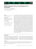
Comparison Simulation results over Zipfian dis-
tributed data can be seen in Fig. 3, which shows the
use of reservoir counting in Online Locality Sensi-
tive Hashing (as made explicit in Algorithm 2), as
compared to the method described by Van Durme
and Lall (2010).
The total amount of space required when using
this counting scheme is b log
2
(k + 1) + 32: b reser-
voirs, and a 32 bit integer to track n. This is com-
pared to b 32 bit floating point values, as is standard.
Note that our scheme comes away with similar lev-
els of accuracy, often at half the memory cost, while
requiring larger b to account for the chance of ap-
proximation errors in individual reservoir counters.
Expected
True
50
100
150
200
250
50 100 150 200 250
Figure 2: Results of simulating many iterations of U


,
for k = 255, and various values of s and u.
Algorithm 1 RESERVOIRUPDATE(n, k, m, σ, s)
Parameters:
n : size of stream so far
k : size of reservoir, also maximum value of s
m : magnitude of update
σ : sign of update
s : current value of reservoir
1: if m = 0 or σ = 0 then
2: Return without doing anything
3: a := A

(m, n, k) = k log
e

n+m
n

4: u := a with probability a − a, a otherwise
5: if σ = 1 then
6: s

:= U

(s, a) = k + (s − k) (1 − 1/k)
u
7: else
8: s


:= U

(s, a) = s (1 − 1/k)
u
9: Return s

 with probability s

− s

, s

 otherwise
Bits.Required
Mean.Absolute.Error
0.06
0.07
0.08
0.09
0.10
0.11
0.12
●
●
●
●
●
●
●

●
●
●
●
1000 2000 3000 4000 5000 6000 7000 8000
log2.k
●
8
●
32
b
●
64
128
192
256
512
Figure 3: Online LSH using reservoir counting (red) vs.
standard counting mechanisms (blue), as measured by the
amount of total memory required to the resultant error.
21
Algorithm 2 COMPUTESIGNATURE(S,k,b,p)
Parameters:
S : bit array of size b
k : size of each reservoir
b : number of projections
p : percentage of zeros in projection, p ∈ [0, 1]
1: Initialize b reservoirs R[1, . . ., b], each represented
by a log
2

(k + 1)-bit unsigned integer
2: Initialize b hash functions h
i
(w) that map features w
to elements in a vector made up of −1 and 1 each
with proportion
1−p
2
, and 0 at proportion p.
3: n := 0
4: {Processing the stream}
5: for each feature value pair (w, m) in stream do
6: for i := 1 to b do
7: R[i] := ReservoirUpdate(n, k, m, h
i
(w), R[i])
8: n := n + m(1 − p)
9: n := n+1 with probability m(1−p)−m(1−p)
10: {Post-processing to compute signature}
11: for i := 1 . . . b do
12: if R[i] >
k
2
then
13: S[i] := 1
14: else
15: S[i] := 0
3 Discussion
Time and Space While we have provided a con-
stant time, approximate update mechanism, the con-

stants involved will practically remain larger than
the cost of performing single hardware addition
or subtraction operations on a traditional 32-bit
counter. This leads to a tradeoff in space vs. time,
where a high-throughput streaming application that
is not concerned with online memory requirements
will not have reason to consider the developments in
this article. The approach given here is motivated
by cases where data is not flooding in at breakneck
speed, and resource considerations are dominated by
a large number of unique elements for which we
are maintaining signatures. Empirically investigat-
ing this tradeoff is a matter of future work.
Random Walks As we here only care for the sign
of the online sum, rather than an approximation of
its actual value, then it is reasonable to consider in-
stead modeling the problem directly as a random
walk on a linear Markov chain, with unit updates
directly corresponding to forward or backward state
-4 -3 -2 -1 0 1 2 3
Figure 4: A simple 8-state Markov chain, requiring
lg(8) = 3 bits. Dark or light states correspond to a
prediction of a running sum being positive or negative.
States are numerically labeled to reflect the similarity to
a small bit integer data type, one that never overflows.
transitions. Assuming a fixed probability of a posi-
tive versus negative update, then in expectation the
state of the chain should correspond to the sign.
However if we are concerned with the global statis-
tic, as we are here, then the assumption of a fixed

probability update precludes the analysis of stream-
ing sources that contain local irregularities.
9
In distributional semantics, consider a feature
stream formed by sequentially reading the n-gram
resource of Brants and Franz (2006). The pair: (the
dog : 3,502,485), can be viewed as a feature value
pair: (leftWord=’the’ : 3,502,485), with respect to
online signature generation for the word dog. Rather
than viewing this feature repeatedly, spread over a
large corpus, the update happens just once, with
large magnitude. A simple chain such as seen in
Fig. 4 will be “pushed” completely to the right or
the left, based on the polarity of the projection, irre-
spective of previously observed updates. Reservoir
Counting, representing an online uniform sample, is
agnostic to the ordering of elements in the stream.
4 Conclusion
We have presented a novel approximation scheme
we call Reservoir Counting, motivated here by a de-
sire for greater space efficiency in Online Locality
Sensitive Hashing. Going beyond our results pro-
vided for synthetic data, future work will explore ap-
plications of this technique, such as in experiments
with streaming social media like Twitter.
Acknowledgments
This work benefited from conversations with Daniel
ˇ
Stefonkovi
ˇ

c and Damianos Karakos.
9
For instance: (1,1, ,1,1,-1,-1,-1), is overall positive, but
locally negative at the end.
22
References
Dimitris Achlioptas. 2003. Database-friendly random
projections: Johnson-lindenstrauss with binary coins.
J. Comput. Syst. Sci., 66:671–687, June.
Shane Bergsma and Benjamin Van Durme. 2011. Learn-
ing Bilingual Lexicons using the Visual Similarity of
Labeled Web Images. In Proc. of the International
Joint Conference on Artificial Intelligence (IJCAI).
Rahul Bhagat and Deepak Ravichandran. 2008. Large
Scale Acquisition of Paraphrases for Learning Surface
Patterns. In Proc. of the Annual Meeting of the Asso-
ciation for Computational Linguistics (ACL).
Thorsten Brants and Alex Franz. 2006. Web 1T 5-gram
version 1.
Moses Charikar. 2002. Similarity estimation techniques
from rounding algorithms. In Proceedings of STOC.
Michel X. Goemans and David P. Williamson. 1995.
Improved approximation algorithms for maximum cut
and satisfiability problems using semidefinite pro-
gramming. JACM, 42:1115–1145.
Amit Goyal, Jagadeesh Jagarlamudi, Hal Daum
´
e III, and
Suresh Venkatasubramanian. 2010. Sketch Tech-
niques for Scaling Distributional Similarity to the

Web. In Proceedings of the ACL Workshop on GEo-
metrical Models of Natural Language Semantics.
Piotr Indyk and Rajeev Motwani. 1998. Approximate
nearest neighbors: towards removing the curse of di-
mensionality. In Proceedings of STOC.
Ping Li, Trevor J. Hastie, and Kenneth W. Church. 2006.
Very sparse random projections. In Proceedings of
the 12th ACM SIGKDD international conference on
Knowledge discovery and data mining, KDD ’06,
pages 287–296, New York, NY, USA. ACM.
Ping Li, Kenneth W. Church, and Trevor J. Hastie. 2008.
One Sketch For All: Theory and Application of Con-
ditional Random Sampling. In Proc. of the Confer-
ence on Advances in Neural Information Processing
Systems (NIPS).
Dekang Lin, Kenneth Church, Heng Ji, Satoshi Sekine,
David Yarowsky, Shane Bergsma, Kailash Patil, Emily
Pitler, Rachel Lathbury, Vikram Rao, Kapil Dalwani,
and Sushant Narsale. 2010. New Tools for Web-Scale
N-grams. In Proceedings of LREC.
Patrick Pantel, Eric Crestan, Arkady Borkovsky, Ana-
Maria Popescu, and Vishnu Vyas. 2009. Web-Scale
Distributional Similarity and Entity Set Expansion. In
Proc. of the Conference on Empirical Methods in Nat-
ural Language Processing (EMNLP).
Sasa Petrovic, Miles Osborne, and Victor Lavrenko.
2010. Streaming First Story Detection with applica-
tion to Twitter. In Proceedings of the Annual Meeting
of the North American Association of Computational
Linguistics (NAACL).

Deepak Ravichandran, Patrick Pantel, and Eduard Hovy.
2005. Randomized Algorithms and NLP: Using Lo-
cality Sensitive Hash Functions for High Speed Noun
Clustering. In Proc. of the Annual Meeting of the As-
sociation for Computational Linguistics (ACL).
Benjamin Van Durme and Ashwin Lall. 2009. Streaming
Pointwise Mutual Information. In Proc. of the Confer-
ence on Advances in Neural Information Processing
Systems (NIPS).
Benjamin Van Durme and Ashwin Lall. 2010. Online
Generation of Locality Sensitive Hash Signatures. In
Proc. of the Annual Meeting of the Association for
Computational Linguistics (ACL).
Jeffrey S. Vitter. 1985. Random sampling with a reser-
voir. ACM Trans. Math. Softw., 11:37–57, March.
23