Tài liệu Báo cáo khoa học: "Generalized Expectation Criteria for Semi-Supervised Learning of Conditional Random Fields" pdf

Proceedings of ACL-08: HLT, pages 870–878,
Columbus, Ohio, USA, June 2008.
c
2008 Association for Computational Linguistics
Generalized Expectation Criteria for Semi-Supervised Learning of
Conditional Random Fields
Gideon S. Mann
Google Inc.
76 Ninth Avenue
New York, NY 10011
Andrew McCallum
Department of Computer Science
University of Massachusetts
140 Governors Drive
Amherst, MA 01003
Abstract
This paper presents a semi-supervised train-
ing method for linear-chain conditional ran-
dom fields that makes use of labeled features
rather than labeled instances. This is accom-
plished by using generalized expectation cri-
teria to express a preference for parameter set-
tings in which the model’s distribution on un-
labeled data matches a target distribution. We
induce target conditional probability distribu-
tions of labels given features from both anno-
tated feature occurrences in context and ad-
hoc feature majority label assignment. The
use of generalized expectation criteria allows
for a dramatic reduction in annotation time
by shifting from traditional instance-labeling

to feature-labeling, and the methods presented
outperform traditional CRF training and other
semi-supervised methods when limited human
effort is available.
1 Introduction
A significant barrier to applying machine learning
to new real world domains is the cost of obtaining
the necessary training data. To address this prob-
lem, work over the past several years has explored
semi-supervised or unsupervised approaches to the
same problems, seeking to improve accuracy with
the addition of lower cost unlabeled data. Tradi-
tional approaches to semi-supervised learning are
applied to cases in which there is a small amount of
fully labeled data and a much larger amount of un-
labeled data, presumably from the same data source.
For example, EM (Nigam et al., 1998), transduc-
tive SVMs (Joachims, 1999), entropy regularization
(Grandvalet and Bengio, 2004), and graph-based
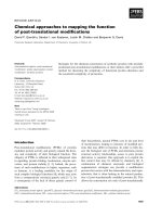
address : *number* oak avenue rent $
ADDRESS ADDRESS
ADDRESS ADDRESS
ADDRESS
RENT
RENT
Traditional Full Instance Labeling
ADDRESS
address : *number* oak avenue rent $
CONTACT
( please include the address of this rental )

ADDRESS
pm . address : *number* marie street sausalito
ADDRESS
laundry . address : *number* macarthur blvd
Feature Labeling
Conditional
Distribution
of Labels
Given
Word=address
ADDRESS
CONTACT
Figure 1: Top: Traditional instance-labeling in which se-
quences of contiguous tokens are annotated as to their
correct label. Bottom: Feature-labeling in which non-
contiguous feature occurrences in context are labeled for
the purpose of deriving a conditional probability distribu-
tion of labels given a particular feature.
methods (Zhu and Ghahramani, 2002; Szummer and
Jaakkola, 2002) have all been applied to a limited
amount of fully labeled data in conjunction with un-
labeled data to improve the accuracy of a classifier.
In this paper, we explore an alternative approach
in which, instead of fully labeled instances, the
learner has access to labeled features. These fea-
tures can often be labeled at a lower-cost to the hu-
man annotator than labeling entire instances, which
may require annotating the multiple sub-parts of a
sequence structure or tree. Features can be labeled
either by specifying the majority label for a partic-

ular feature or by annotating a few occurrences of
a particular feature in context with the correct label
(Figure 1).
To train models using this information we use
870
generalized expectation (GE) criteria. GE criteria
are terms in a training objective function that as-
sign scores to values of a model expectation. In
particular we use a version of GE that prefers pa-
rameter settings in which certain model expectations
are close to target distributions. Previous work has
shown how to apply GE criteria to maximum en-
tropy classifiers. In section 4, we extend GE crite-
ria to semi-supervised learning of linear-chain con-
ditional random fields, using conditional probability
distributions of labels given features.
To empirically evaluate this method we compare
it with several competing methods for CRF train-
ing, including entropy regularization and expected
gradient, showing that GE provides significant im-
provements. We achieve competitive performance
in comparison to alternate model families, in partic-
ular generative models such as MRFs trained with
EM (Haghighi and Klein, 2006) and HMMs trained
with soft constraints (Chang et al., 2007). Finally, in
Section 5.3 we show that feature-labeling can lead to
dramatic reductions in the annotation time that is re-
quired in order to achieve the same level of accuracy
as traditional instance-labeling.
2 Related Work

There has been a significant amount of work on
semi-supervised learning with small amounts of
fully labeled data (see Zhu (2005)). However there
has been comparatively less work on learning from
alternative forms of labeled resources. One exam-
ple is Schapire et al. (2002) who present a method
in which features are annotated with their associated
majority labels and this information is used to boot-
strap a parameterized text classification model. Un-
like the model presented in this paper, they require
some labeled data in order to train their model.
This type of input information (features + major-
ity label) is a powerful and flexible model for spec-
ifying alternative inputs to a classifier, and has been
additionally used by Haghighi and Klein (2006). In
that work, “prototype” features—words with their
associated labels—are used to train a generative
MRF sequence model. Their probability model can
be formally described as:
p
θ
(x, y) =
1
Z(θ)
exp


k
θ
k

F
k
(x, y)

.
Although the partition function must be computed
over all (x, y) tuples, learning via EM in this model
is possible because of approximations made in com-
puting the partition function.
Another way to gather supervision is by means
of prior label distributions. Mann and McCallum
(2007) introduce a special case of GE, label regular-
ization, and demonstrate its effectiveness for train-
ing maximum entropy classifiers. In label regu-
larization, the model prefers parameter settings in
which the model’s predicted label distribution on the
unsupervised data match a target distribution. Note
that supervision here consists of the the full distribu-
tion over labels (i.e. conditioned on the maximum
entropy “default feature”), instead of simply the ma-
jority label. Druck et al. (2007) also use GE with full
distributions for semi-supervised learning of maxi-
mum entropy models, except here the distributions
are on labels conditioned on features. In Section 4
we describe how GE criteria can be applied to CRFs
given conditional probability distributions of labels
given features.
Another recent method that has been proposed for
training sequence models with constraints is Chang
et al. (2007). They use constraints for approximate

EM training of an HMM, incorporating the con-
straints by looking only at the top K most-likely
sequences from a joint model of likelihood and the
constraints. This model can be applied to the combi-
nation of labeled and unlabeled instances, but cannot
be applied in situations where only labeled features
are available. Additionally, our model can be easily
combined with other semi-supervised criteria, such
as entropy regularization. Finally, their model is a
generative HMM which cannot handle the rich, non-
independent feature sets that are available to a CRF.
There have been relatively few different ap-
proaches to CRF semi-supervised training. One ap-
proach has been that proposed in both Miller et al.
(2004) and Freitag (2004), uses distributional clus-
tering to induce features from a large corpus, and
then uses these features to augment the feature space
of the labeled data. Since this is an orthogonal
method for improving accuracy it can be combined
with many of the other methods discussed above,
and indeed we have obtained positive preliminary
experimental results with GE criteria (not reported
on here).
871
Another method for semi-supervised CRF train-
ing is entropy regularization, initially proposed by
Grandvalet and Bengio (2004) and extended to
linear-chain CRFs by Jiao et al. (2006). In this for-
mulation, the traditional label likelihood (on super-
vised data) is augmented with an additional term that

encourages the model to predict low-entropy label
distributions on the unlabeled data:
O(θ; D, U) =

d
log p
θ
(y
(d)
|x
(d)
) − λH(y|x).
This method can be quite brittle, since the minimal
entropy solution assigns all of the tokens the same
label.
1
In general, entropy regularization is fragile,
and accuracy gains can come only with precise set-
tings of λ. High values of λ fall into the minimal
entropy trap, while low values of λ have no effect on
the model (see (Jiao et al., 2006) for an example).
When some instances have partial labelings (i.e.
labels for some of their tokens), it is possible to train
CRFs via expected gradient methods (Salakhutdinov
et al., 2003). Here a reformulation is presented in
which the gradient is computed for a probability dis-
tribution with a marginalized hidden variable, z, and
observed training labels y:
∇
L

(θ) =
∂
∂θ

z
log p(x, y, z; θ)
=

z
p(z|y, x)f
k
(x, y, z)
−

z,y

p(z, y

|x; θ)f
k
(x, y, z).
In essence, this resembles the standard gradient for
the CRF, except that there is an additional marginal-
ization in the first term over the hidden variable z.
This type of training has been applied by Quattoni
et al. (2007) for hidden-state conditional random
fields, and can be equally applied to semi-supervised
conditional random fields. Note, however, that la-
beling variables of a structured instance (e.g. to-
kens) is different than labeling features—being both

more coarse-grained and applying supervision nar-
rowly only to the individual subpart, not to all places
in the data where the feature occurs.
1
In the experiments in this paper, we use λ = 0.001, which
we tuned for best performance on the test set, giving an unfair
advantage to our competitor.
Finally, there are some methods that use auxil-
iary tasks for training sequence models, though they
do not train linear-chain CRFs per se. Ando and
Zhang (2005) include a cluster discovery step into
the supervised training. Smith and Eisner (2005)
use neighborhoods of related instances to figure out
what makes found instances “good”. Although these
methods can often find good solutions, both are quite
sensitive to the selection of auxiliary information,
and making good selections requires significant in-
sight.
2
3 Conditional Random Fields
Linear-chain conditional random fields (CRFs) are a
discriminative probabilistic model over sequences x
of feature vectors and label sequences y = y
1
y
n
,
where |x| = |y| = n, and each label y
i
has s dif-

ferent possible discrete values. This model is anal-
ogous to maximum entropy models for structured
outputs, where expectations can be efficiently calcu-
lated by dynamic programming. For a linear-chain
CRF of Markov order one:
p
θ
(y|x) =
1
Z(x)
exp


k
θ
k
F
k
(x, y)

,
where F
k
(x, y) =

i
f
k
(x, y
i

, y
i+1
, i),
and the partition function Z(x) =

y
exp(

k
θ
k
F
k
(x, y)). Given training data
D =

(x
(1)
, y
(1)
) (x
(n)
, y
(n)
)

, the model is tra-
ditionally trained by maximizing the log-likelihood
O(θ; D) =


d
log p
θ
(y
(d)
|x
(d)
) by gradient ascent
where the gradient of the likelihood is:
∂
∂θ
k
O(θ; D) =

d
F
k
(x
(d)
, y
(d)
)
−

d

y
p
θ
(y|x

(d)
)F
k
(x
(d)
, y).
The second term (the expected counts of the features
given the model) can be computed in a tractable
amount of time, since according to the Markov as-
2
Often these are more complicated than picking informative
features as proposed in this paper. One example of the kind of
operator used is the transposition operator proposed by Smith
and Eisner (2005).
872
sumption, the feature expectations can be rewritten:

y
p
θ
(y|x)F
k
(x, y) =

i

y
i
,y
i+1

p
θ
(y
i
, y
i+1
|x)f
k
(x, y
i
, y
i+1
, i).
A dynamic program (the forward/backward algo-
rithm) then computes in time O(ns
2
) all the needed
probabilities p
θ
(y
i
, y
i+1
), where n is the sequence
length, and s is the number of labels.
4 Generalized Expectation Criteria for
Conditional Random Fields
Prior semi-supervised learning methods have aug-
mented a limited amount of fully labeled data with
either unlabeled data or with constraints (e.g. fea-

tures marked with their majority label). GE crite-
ria can use more information than these previous
methods. In particular GE criteria can take advan-
tage of conditional probability distributions of la-
bels given a feature (p(y|f
k
(x) = 1)). This in-
formation provides richer constraints to the model
while remaining easily interpretable. People have
good intuitions about the relative predictive strength
of different features. For example, it is clear that
the probability of label PERSON given the feature
WORD=JOHN is high, perhaps around 0.95, where
as for WORD=BROWN it would be lower, perhaps
0.4. These distributions need not be not estimated
with great precision—it is far better to have the free-
dom to express shades of gray than to be force into
a binary supervision signal. Another advantage of
using conditional probability distributions as prob-
abilistic constraints is that they can be easily esti-
mated from data. For the feature INITIAL-CAPITAL,
we identify all tokens with the feature, and then
count the labels with which the feature co-occurs.
GE criteria attempt to match these conditional
probability distributions by model expectations on
unlabeled data, encouraging, for example, the model
to predict that the proportion of the label PERSON
given the word “john” should be .95 over all of the
unlabeled data.
In general, a GE (generalized expectation) crite-

rion (McCallum et al., 2007) expresses a preference
on the value of a model expectation. One kind of
preference may be expressed by a distance function
∆, a target expectation
ˆ
f, data D, a function f , and
a model distribution p
θ
, the GE criterion objective
function term is ∆

ˆ
f, E[f(x)]

. For the purposes
of this paper, we set the functions to be conditional
probability distributions and set ∆(p, q) = D(p||q),
the KL-divergence between two distributions.
3
For
semi-supervised training of CRFs, we augment the
objective function with the regularization term:
O(θ; D, U) =

d
log p
θ
(y
(d)
|x

(d)
) −

k
θ
k
2σ
2
− λD(ˆp||˜p
θ
),
where ˆp is given as a target distribution and
˜p
θ
= ˜p
θ
(y
j
|f
m
(x, j) = 1)
=
1
U
m

x∈U
m

j


p
θ
(y

j
|x),
with the unnormalized potential
˜q
θ
= ˜q
θ
(y
j
|f
m
(x, j) = 1) =

x∈U
m

j

p
θ
(y

j
|x),
where f

m
(x, j) is a feature that depends only on
the observation sequence x, and j

is defined as
{j : f
m
(x, j) = 1}, and U
m
is the set of sequences
where f
m
(x, j) is present for some j.
4
Computing the Gradient
To compute the gradient of the GE criteria,
D(ˆp||˜p
θ
), first we drop terms that are constant with
respect to the partial derivative, and we derive the
gradient as follows:
∂
∂θ
k

l
ˆp log ˜q
θ
=


l
ˆp
˜q
θ
∂
∂θ
k
˜q
θ
=

l
ˆp
˜q
θ

x∈U

j

∂
∂θ
k
p
θ
(y
j

= l|x)
=


l
ˆp
˜q
θ

x∈U

j


y
−j

∂
∂θ
k
p
θ
(y
j

= l, y
−j

|x),
where y
−j
= y
1 (j−1)

y
(j+1) n
. The last step fol-
lows from the definition of the marginal probability
3
We are actively investigating different choices of distance
functions which may have different generalization properties.
4
This formulation assumes binary features.
873
P (y
j
|x). Now that we have a familiar form in which
we are taking the gradient of a particular label se-
quence, we can continue:
=

l
ˆp
˜q
θ

x∈U

j


y
−j


p
θ
(y
j

= l, y
−j

|x)F
k
(x, y)
−

l
ˆp
˜q
θ

x∈U

j


y
−j

p
θ
(y
j


= l, y
−j

|x)

y

p
θ
(y

|x)F
k
(x, y)
=

l
ˆp
˜q
θ

x∈U

i

y
i
,y
i+1

f
k
(x, y
i
, y
i+1
, i)

j

p
θ
(y
i
, y
i+1
, y
j

= l|x)
−

l
ˆp
˜q
θ

x∈U

i


y
i
,y
i+1
f
k
(x, y
i
, y
i+1
, i)
p
θ
(y
i
, y
i+1
|x)

j

p
θ
(y
j

= l|x).
After combining terms and rearranging we arrive at
the final form of the gradient:

=

x∈U

i

y
i
,y
i+1
f
k
(x, y
i
, y
i+1
, i)

l
ˆp
˜q
θ
×


j

p
θ
(y

i
, y
i+1
, y
j

= l|x)−
p
θ
(y
i
, y
i+1
|x)

j

p
θ
(y
j

= l|x)

.
Here, the second term is easily gathered from for-
ward/backward, but obtaining the first term is some-
what more complicated. Computing this term
naively would require multiple runs of constrained
forward/backward. Here we present a more ef-

ficient method that requires only one run of for-
ward/backward.
5
First we decompose the prob-
ability into two parts:

j

p
θ
(y
i
, y
i+1
, y
j

=
l|x) =

i
j=1
p
θ
(y
i
, y
i+1
, y
j

= l|x)I(j ∈ j

) +

J
j=i+1
p
θ
(y
i
, y
i+1
, y
j
= l|x)I(j ∈ j

). Next, we
show how to compute these terms efficiently. Simi-
lar to forward/backward, we build a lattice of inter-
mediate results that then can be used to calculate the
5
(Kakade et al., 2002) propose a related method that com-
putes p(y
1 i
= l
1 i
|y
i+1
= l).
quantity of interest:

i

j=1
p
θ
(y
i
, y
i+1
, y
j
= l|x)I(j ∈ j

)
= p(y
i
, y
i+1
|x)δ(y
i
, l)I(i ∈ j

)
+
i−1

j=1
p
θ
(y

i
, y
i+1
, y
j
= l|x)I(j ∈ j

)
= p(y
i
, y
i+1
|x)δ(y
i
, l)I(i ∈ j

)
+



y
i−1
i−1

j=1
p
θ
(y
i−1

, y
i
, y
j
= l|x)I(j ∈ j

)


p
θ
(y
i+1
|y
i
, x).
For efficiency,

y
i−1

i−1
j=1
p
θ
(y
i−1
, y
i
, y

j
=
l|x)I(j ∈ j

) is saved at each stage in the lat-
tice.

J
j=i+1
p
θ
(y
i−1
, y
i
, y
j
= l|x)I(j ∈ j

) can
be computed in the same fashion. To compute the
lattices it takes time O(ns
2
), and one lattice must be
computed for each label so the total time is O(ns
3
).
5 Experimental Results
We use the CLASSIFIEDS data provided by Grenager
et al. (2005) and compare with results reported

by HK06 (Haghighi and Klein, 2006) and CRR07
(Chang et al., 2007). HK06 introduced a set of 33
features along with their majority labels, these are
the primary set of additional constraints (Table 1).
As HK06 notes, these features are selected using
statistics of the labeled data, and here we used sim-
ilar features here in order to compare with previous
results. Though in practice we have found that fea-
ture selection is often intuitive, recent work has ex-
perimented with automatic feature selection using
LDA (Druck et al., 2008). For some of the exper-
iments we also use two sets of 33 additional fea-
tures that we chose by the same method as HK06,
the first 33 of which are also shown in Table 1. We
use the same tokenization of the dataset as HK06,
and training/test/unsupervised sets of 100 instances
each. This data differs slightly from the tokenization
used by CRR07. In particular it lacks the newline
breaks which might be a useful piece of information.
There are three types of supervised/semi-
supervised data used in the experiments. Labeled
instances are the traditional or conventionally
874
Label HK06: 33 Features 33 Added Features
CONTACT *phone* call *time please appointment more
FEATURES kitchen laundry parking room new large
ROOMMATES roommate respectful drama i bit mean
RESTRICTIONS pets smoking dog no sorry cats
UTILITIES utilities pays electricity water garbage included
AVAILABLE immediately begin cheaper *month* now *ordinal*0

SIZE *number*1*1 br sq *number*0*1 bedroom bath
PHOTOS pictures image link *url*long click photos
RENT *number*15*1 $ month deposit lease rent
NEIGHBORHOOD close near shopping located bart downtown
ADDRESS address carlmont ave san *ordinal*5 #
Table 1: Features and their associated majority label.
Features for each label were chosen by the method de-
scribed in HK06 – top frequency for that label and not
higher frequency for any other label.
+ SVD features
HK06 53.7% 71.5%
CRF + GE/Heuristic 66.9% 68.3%
Table 2: Accuracy of semi-supervised learning methods
with majority labeled features alone. GE outperforms
HK06 when neither model has access to SVD features.
When SVD features are included, HK06 has an edge in
accuracy.
labeled instances used for estimation in traditional
CRF training. Majority labeled features are fea-
tures annotated with their majority label.
6
Labeled
features are features m where the distribution
p(y
i
|f
m
(x, i)) has been specified. In Section 5.3 we
estimate these distributions from isolated labeled
tokens.

We evaluate the system in two scenarios: (1) with
feature constraints alone and (2) feature constraints
in conjunction with a minimal amount of labeled in-
stances. There is little prior work that demonstrates
the use of both scenarios; CRR07 can only be ap-
plied when there is some labeled data, while HK06
could be applied in both scenarios though there are
no such published experiments.
5.1 Majority Labeled Features Only
When using majority labeled features alone, it can
be seen in Table 2 that GE is the best performing
method. This is important, as it demonstrates that
GE out of the box can be used effectively, without
tuning and extra modifications.
6
While HK06 and CRR07 require only majority labeled fea-
tures, GE criteria use conditional probability distributions of la-
bels given features, and so in order to apply GE we must decide
on a particular distribution for each feature constraint. In sec-
tions 5.1 and 5.2 we use a simple heuristic to derive distribu-
tions from majority label information: we assign .99 probabil-
ity to the majority label of the feature and divide the remaining
probability uniformly among the remainder of the labels.
Labeled Instances
10 25 100
supervised HMM 61.6% 70.0% 76.3%
supervised CRF 64.6% 72.9% 79.4%
CRF+ Entropy Reg. 67.3% 73.7% 79.5%
CRR07 70.9% 74.8% 78.6%
+ inference constraints 74.7% 78.5% 81.7%

CRF+GE/Heuristic 72.6% 76.3% 80.1%
Table 3: Accuracy of semi-supervised learning meth-
ods with constraints and limited amounts of training
data. Even though CRR07 uses more constraints and re-
quires additional development data for estimating mix-
ture weights, GE still outperforms CRR07 when that sys-
tem is run without applying constraints during inference.
When these constraints are applied during test-time infer-
ence, CRR07 has an edge over the CRF trained with GE
criteria.
In their original work, HK06 propose a method
for generating additional features given a set of “pro-
totype” features (the feature constraints in Table 1),
which they demonstrate to be highly effective. In
their method, they collect contexts around all words
in the corpus, then perform a SVD decomposition.
They take the first 50 singular values for all words,
and then if a word is within a thresholded distance
to a prototype feature, they assign that word a new
feature which indicates close similarity to a proto-
type feature. When SVD features such as these are
made available to the systems, HK06 has a higher
accuracy.
7
For the remainder of the experiments we
use the SVD feature enhanced data sets.
8
We ran additional experiments with expected gra-
dient methods but found them to be ineffective,
reaching around 50% accuracy on the experiments

with the additional SVD features, around 20% less
than the competing methods.
5.2 Majority Labeled Features and Labeled
Instances
Labeled instances are available, the technique de-
scribed in CRR07 can be used. While CRR07 is
run on the same data set as used by HK06, a direct
comparison is problematic. First, they use additional
constraints beyond those used in this paper and those
7
We generated our own set of SVD features, so they might
not match exactly the SVD features described in HK06.
8
One further experiment HK06 performs which we do not
duplicate here is post-processing the label assignments to better
handle field boundaries. With this addition they realize another
2.5% improvement.
875
used by HK06 (e.g. each contiguous label sequence
must be at least 3 labels long)—so their results can-
not be directly compared. Second, they require addi-
tional training data to estimate weights for their soft
constraints, and do not measure how much of this
additional data is needed. Third, they use a slightly
different tokenization procedure. Fourth, CRR07
uses different subsets of labeled training instances
than used here. For these reasons, the comparison
between the method presented here and CRR07 can-
not be exact.
The technique described in CRR07 can be applied

in two ways: constraints can be applied during learn-
ing, and they can also be applied during inference.
We present comparisons with both of these systems
in Table 3. CRFs trained with GE criteria consis-
tently outperform CRR07 when no constraints are
applied during inference time, even though CRR07
has additional constraints. When the method in
CRR07 is applied with constraints in inference time,
it is able to outperform CRFs trained with GE. We
tried adding the additional constraints described in
CRR07 during test-time inference in our system, but
found no accuracy improvement. After doing error
inspection, those additional constraints weren’t fre-
quently violated by the GE trained method, which
also suggests that adding them wouldn’t have a sig-
nificant effect during training either. It is possible
that for GE training there are alternative inference-
time constraints that would improve performance,
but we didn’t pursue this line of investigation as
there are benefits to operating within a formal prob-
abilistic model, and eschewing constraints applied
during inference time. Without these constraints,
probabilistic models can be combined easily with
one another in order to arrive at a joint model, and
adding in these constraints at inference time compli-
cates the nature of the combination.
5.3 Labeled Features vs. Labeled Instances
In the previous section, the supervision signal was
the majority label of each feature.
9

Given a feature
of interest, a human can gather a set of tokens that
have this feature and label them to discover the cor-
9
It is not clear how these features would be tagged with ma-
jority label in a real use case. Tagging data to discover the ma-
jority label could potentially require a large number of tagged
instances before the majority label was definitively identified.
Accuracy
Tokens
0.45
0.5
0.55
0.6
0.65
0.7
0.75
0.8
0.85
10 100 1000 10000 100000
Traditional Instance Labeling
33 Labeled Features
66 Labeled Features
99 Labeled Features
CRR07 + inference time constraints
Figure 2: Accuracy of supervised and semi-supervised
learning methods for fixed numbers of labeled tokens.
Training a GE model with only labeled features sig-
nificantly outperforms traditional log-likelihood training
with labeled instances for comparable numbers of labeled

tokens. When training on less than 1500 annotated to-
kens, it also outperforms CRR07 + inference time con-
straints, which uses not only labeled tokens but additional
constraints and development data for estimating mixture
weights.
Labeled Instances
0 10 25 100
HK06 71.5% - - -
GE/Heuristic 68.3% 72.6% 76.3% 80.1%
GE/Sampled 73.0% 74.6% 77.2% 80.5%
Table 4: Accuracy of semi-supervised learning methods
comparing the effects of (1) a heuristic for setting con-
ditional distributions of labels given features and (2) es-
timating this distributions via human annotation. When
GE is given feature distributions are better than the sim-
ple heuristic it is able to realize considerable gains.
relation between the feature and the labels.
10
While
the resulting label distribution information could not
be fully utilized by previous methods (HK06 and
CRR07 use only the majority label of the word), it
can, however, be integrated into the GE criteria by
using the distribution from the relative proportions
of labels rather than a the previous heuristic distri-
bution. We present a series of experiments that test
the advantages of this annotation paradigm.
To simulate a human labeler, we randomly sam-
ple (without replacement) tokens with the particu-
lar feature in question, and generate a label using

the human annotations provided in the data. Then
we normalize and smooth the raw counts to obtain a
10
In this paper we observe a 10x speed-up by using isolated
labeled tokens instead of a wholly labeled instances—so even
if it takes slightly longer to label isolated tokens, there will still
be a substantial gain.
876
conditional probability distribution over labels given
feature. We experiment with samples of 1, 2,5, 10,
100 tokens per feature, as well as with all available
labeled data. We sample instances for labeling ex-
clusively from the training and development data,
not from the testing data. We train a model using GE
with these estimated conditional probability distri-
butions and compare them with corresponding num-
bers of tokens of traditionally labeled instances.
Training from labeled features significantly out-
performs training from traditional labeled instances
for equivalent numbers of labeled tokens (Figure
2). With 1000 labeled tokens, instance-labeling
achieves accuracy around 65%, while labeling 33
features reaches 72% accuracy.
11
To achieve the
same level of performance as traditional instance la-
beling, it can require as much as a factor of ten-fold
fewer annotations of feature occurrences. For exam-
ple, the accuracy achieved after labeling 257 tokens
of 33 features is 71% – the same accuracy achieved

only after labeling more than 2000 tokens in tradi-
tional instance-labeling.
12
Assuming that labeling one token in isolation
takes the same time as labeling one token in a
sequence, these results strongly support a new
paradigm of labeling in which instead of annotat-
ing entire sentences, the human instead selects some
key features of interest and labels tokens that have
this feature. Particularly intriguing is the flexibility
our scenario provides for the selection of “features
of interest” to be driven by error analysis.
Table 4 compares the heuristic method described
above against sampled conditional probability distri-
butions of labels given features
13
. Sampled distribu-
tions yield consistent improvements over the heuris-
tic method. The accuracy with no labeled instances
(73.0%) is better than HK06 (71.5%), which demon-
strates that the precisely estimated feature distribu-
tions are helpful for improving accuracy.
Though accuracy begins to level off with distri-
11
Labeling 99 features with 1000 tokens reaches nearly 76%.
12
Accuracy at one labeled token per feature is much worse
than accuracy with majority label information. This due to the
noise introduced by sampling, as there is the potential for a rel-
atively rare label be sampled and labeled, and thereby train the

system on a non-canonical supervision signal.
13
Where the tokens labeled is the total available number in
the data, roughly 2500 tokens.
0
0.2
0.4
0.6
0.8
1
0 2 4 6 8 10 12
Probability
Label
0
0.2
0.4
0.6
0.8
1
0 2 4 6 8 10 12
Probability
Label
Figure 3: From left to right: distributions (with standard
error) for the feature WORD=ADDRESS obtained from
sampling, using 1 sample per feature and 10 samples per
feature. Labels 1, 2, 3, and 9 are (respectively) FEA-
TURES, CONTACT, SIZE, and ADDRESS. Instead of more
precisely estimating these distributions, it is more benefi-
cial to label a larger set of features.
butions over the original set of 33 labeled features,

we ran additional experiments with 66 and 99 la-
beled features, whose results are also shown in Fig-
ure 2.
14
The graph shows that with an increased
number of labeled features, for the same numbers
of labeled tokens, accuracy can be improved. The
reason behind this is clear—while there is some gain
from increased precision of probability estimates (as
they asymptotically approach their “true” values as
shown in Figure 3), there is more information to be
gained from rougher estimates of a larger set of fea-
tures. One final point about these additional features
is that their distributions are less peaked than the
original feature set. Where the original feature set
distribution has entropy of 8.8, the first 33 added fea-
tures have an entropy of 22.95. Surprisingly, even
ambiguous feature constraints are able to improve
accuracy.
6 Conclusion
We have presented generalized expectation criteria
for linear-chain conditional random fields, a new
semi-supervised training method that makes use of
labeled features rather than labeled instances. Pre-
vious semi-supervised methods have typically used
ad-hoc feature majority label assignments as con-
straints. Our new method uses conditional proba-
bility distributions of labels given features and can
dramatically reduce annotation time. When these
distributions are estimated by means of annotated

feature occurrences in context, there is as much as
a ten-fold reduction in the annotation time that is re-
quired in order to achieve the same level of accuracy
over traditional instance-labeling.
14
Also note that for less than 1500 tokens of labeling, the 99
labeled features outperform CRR07 with inference time con-
straints.
877
References
R. K. Ando and T. Zhang. 2005. A framework for learn-
ing predictive structures from multiple tasks and unla-
beled data. JMLR, 6.
M W. Chang, L. Ratinov, and D. Roth. 2007. Guiding
semi-supervision with constraint-driven learning. In
ACL.
G. Druck, G. Mann, and A. McCallum. 2007. Lever-
aging existing resources using generalized expectation
criteria. In NIPS Workshop on Learning Problem De-
sign.
G. Druck, G. S. Mann, and A. McCallum. 2008. Learn-
ing from labeled features using generalized expecta-
tion criteria. In SIGIR.
D. Freitag. 2004. Trained named entity recognition using
distributional clusters. In EMNLP.
Y. Grandvalet and Y. Bengio. 2004. Semi-supervised
learning by entropy minimization. In NIPS.
T. Grenager, D. Klein, and C. Manning. 2005. Unsuper-
vised learning of field segmentation models for infor-
mation extraction. In ACL.

A. Haghighi and D. Klein. 2006. Prototype-driver learn-
ing for sequence models. In NAACL.
F. Jiao, S. Wang, C H. Lee, R. Greiner, and D. Schu-
urmans. 2006. Semi-supervised conditional random
fields for improved sequence segmentation and label-
ing. In COLING/ACL.
Thorsten Joachims. 1999. Transductive inference for
text classification using support vector machines. In
ICML.
S. Kakade, Y-W. Teg, and S.Roweis. 2002. An alternate
objective function for markovian fields. In ICML.
G. Mann and A. McCallum. 2007. Simple, robust, scal-
able semi-supervised learning via expectation regular-
ization. In ICML.
A. McCallum, G. S. Mann, and G. Druck. 2007. Gener-
alized expectation criteria. Computer science techni-
cal note, University of Massachusetts, Amherst, MA.
S. Miller, J. Guinness, and A. Zamanian. 2004. Name
tagging with word clusters and discriminative training.
In ACL.
K. Nigam, A. McCallum, S. Thrun, and T. Mitchell.
1998. Learning to classify text from labeled and un-
labeled documents. In AAAI.
A. Quattoni, S. Wang, L-P. Morency, M. Collins, and
T. Darrell. 2007. Hidden-state conditional random
fields. In PAMI.
H. Raghavan, O. Madani, and R. Jones. 2006. Active
learning with feedback on both features and instances.
JMLR.
R. Salakhutdinov, S. Roweis, and Z. Ghahramani. 2003.

Optimization with em and expectation-conjugate-
gradient. In ICML.
R. Schapire, M. Rochery, M. Rahim, and N. Gupta.
2002. Incorporating prior knowledge into boosting.
In ICML.
N. Smith and J. Eisner. 2005. Contrastive estimation:
Training log-linear models on unlabeled data. In ACL.
Martin Szummer and Tommi Jaakkola. 2002. Partially
labeled classification with markov random walks. In
NIPS, volume 14.
X. Zhu and Z. Ghahramani. 2002. Learning from labeled
and unlabeled data with label propagation. Technical
Report CMU-CALD-02-107, CMU.
X. Zhu. 2005. Semi-supervised learning lit-
erature survey. Technical Report 1530, Com-
puter Sciences, University of Wisconsin-Madison.
survey.pdf.
878