High resolution continuum source AAS the better way to do atomic absorption spectrometry
Bạn đang xem bản rút gọn của tài liệu. Xem và tải ngay bản đầy đủ của tài liệu tại đây (8.03 MB, 310 trang )
www.pdfgrip.com
High-Resolution
Continuum Source AAS
The Better Way to Do Atomic Absorption
Spectrometry
Bernhard Welz, Helmut Becker-Ross,
Stefan Florek, Uwe Heitmann
WILEY-VCH Verlag GmbH & Co. KGaA
www.pdfgrip.com
www.pdfgrip.com
High-Resolution
Continuum Source AAS
B. Welz, H. Becker-Ross,
S. Florek, U. Heitmann
www.pdfgrip.com
Further Titles of Interest:
J. A. C. Broekaert
Analytical Atomic Spectrometry with Flames
and Plasmas
2nd Edition
2005, ISBN 3-527-31282-X
E. Merian, M. Anke, M. Ihnat, M. Stoeppler
Elements and their Compounds in the Environment
Occurrence, Analysis and Biological Relevance
3 Volumes, 2nd Edition
2004, ISBN 3-527-30459-2
J. Nölte
ICP Emission Spectrometry
A Practical Guide
2003, ISBN 3-527-30672-2
B. Welz, M. Sperling
Atomic Absorption Spectrometry
3rd Edition
1999, ISBN 3-527-28571-7
www.pdfgrip.com
High-Resolution
Continuum Source AAS
The Better Way to Do Atomic Absorption
Spectrometry
Bernhard Welz, Helmut Becker-Ross,
Stefan Florek, Uwe Heitmann
WILEY-VCH Verlag GmbH & Co. KGaA
www.pdfgrip.com
Authors
Prof. Dr. Bernhard Welz
Departamento de Química
Universidade Federal de Santa Catarina
88040-900 Florianópolis – SC
Brazil
Dr. Helmut Becker-Ross
ISAS – Institute for Analytical Sciences,
Department Berlin
ISAS – Institute for Analytical Sciences,
Department Berlin
Albert-Einstein-Strasse 9
12489 Berlin
Germany
Dr. Stefan Florek
ISAS – Institute for Analytical Sciences,
Department Berlin
Albert-Einstein-Strasse 9
12489 Berlin
Germany
Dr. Uwe Heitmann
ISAS – Institute for Analytical Sciences,
Department Berlin
Albert-Einstein-Strasse 9
12489 Berlin
Germany
All books published by Wiley-VCH are carefully
produced. Nevertheless, authors, and publisher do
not warrant the information contained in these
books, including this book, to be free of errors.
Readers are advised to keep in mind that statements, data, illustrations, procedural details or
other items may inadvertently be inaccurate.
Library of Congress Card No.: applied for
British Library Cataloging-in-Publication Data:
A catalogue record for this book is available from
the British Library
Bibliographic information published by
Die Deutsche Bibliothek
Die Deutsche Bibliothek lists this publication
in the Deutsche Nationalbibliografie; detailed
bibliographic data is available in the
Internet at <>.
© 2005 WILEY-VCH Verlag GmbH & Co.
KGaA, Weinheim
All rights reserved (including those of translation
into other languages). No part of this book may
be reproduced in any form – nor transmitted or
translated into machine language without written
permission from the publishers. Registered
names, trademarks, etc. used in this book, even
when not specifically marked as such, are not to
be considered unprotected by law.
Printed in the Federal Republic of Germany
Printed on acid-free paper
Printing Druckhaus Darmstadt GmbH,
Darmstadt
Bookbinding Litges & Dopf Buchbinderei
GmbH, Heppenheim
ISBN-13: 978- 3-527-30736-4
ISBN-10: 3-527-30736-2
www.pdfgrip.com
Preface
Conventional line source atomic absorption spectrometry (LS AAS) can nowadays be considered an established technique in the positive sense of the term, i.e. it is widely used, and
no dramatic improvements are expected in the foreseeable future. The state-of-the-art of
conventional LS AAS is fully described in the book of Welz and Sperling [150], and its
content may well be valid for another decade or two. The only progress will be in the
development of new applications, but this field is today fully covered by a variety of data
banks, which are easily accessible through the Internet, so that this increase in literature
on applications does not justify a new edition of this book.
The only real progress in the field of AAS, in the opinion of the authors, is in the direction of high-resolution continuum source AAS (HR-CS AAS), which will undoubtedly
be the future of this technique. For this reason we thought it would be much more useful
to write a new book about HR-CS AAS, which might be considered a ‘Volume 2’ or a
‘Supplement’ of the above basic book on AAS. This means we expect the reader of this
book to be aware of the basic concepts of AAS, which is fully covered in Reference [150],
and so we have deliberately avoided repeating things in this book that have been described
in the former one. For example, neither the different atomizers used in AAS, i.e. flame,
graphite furnace or quartz tube atomizers, nor the atomization mechanisms or the nonspectral interferences occurring in these atomizers are discussed in this book, as they are
obviously identical. In essence, only the new aspects and developments that are particular
to HR-CS AAS are discussed in detail, whereas common things are repeated only where
absolutely necessary.
The content of this book, regarding practical application, has essentially been produced over a time period of less than two years using prototype instruments, which are
similar, but not identical, to the commercially available instrument. There have been an
impressive number of people, master, doctoral and post-doctoral students, working with
these prototypes, but obviously we can only give examples for the application of this new
technique, not a full coverage of all the possibilities. We expect that you, the readers of
this book, who hopefully will be using this exciting new technique, will be contributing
v
www.pdfgrip.com
Preface
to the exploration of the potential of HR-CS AAS so that the second edition of this book
will contain a much more complete coverage of yet undiscovered application possibilities
of this new technique.
This book is an integral part of the professorial dissertation of Uwe Heitmann. He
has written several chapters and was responsible for the preparation of the figures as well
as for the total arrangement and layout of this book up to the delivery of a ready-forpress manuscript. Uwe Heitmann has been concerned with the HR-CS AAS project since
1994. He was involved in most of the measurements, their evaluation and interpretation.
Moreover, he carried out the setup of the prototype instruments and wrote the in-house
software for data acquisition, signal processing and background correction.
Florianópolis, Berlin, December 2004
vi
Bernhard Welz
Helmut Becker-Ross
Stefan Florek
Uwe Heitmann
www.pdfgrip.com
Contents
1. Historical Development of Continuum Source AAS
1
2. Theoretical Concepts
2.1
2.2
2.3
Spectral Line Profiles . . . . . . . . . . . . .
2.1.1 Natural Line Width . . . . . . . . . .
2.1.2 Doppler Broadening . . . . . . . . .
2.1.3 Collision Broadening . . . . . . . . .
2.1.4 Voigt Profiles . . . . . . . . . . . . .
2.1.5 Instrument Profile . . . . . . . . . .
Atomic Absorption with a Continuum Source
2.2.1 General Principle of Absorption . . .
2.2.2 Instrument Effects . . . . . . . . . .
Structure of Molecular Spectra . . . . . . . .
2.3.1 Electronic Transitions . . . . . . . .
2.3.2 Vibrational Spectra . . . . . . . . . .
2.3.3 Rotational Spectra . . . . . . . . . .
2.3.4 Dissociation Continua . . . . . . . .
5
.
.
.
.
.
.
.
.
.
.
.
.
.
.
.
.
.
.
.
.
.
.
.
.
.
.
.
.
.
.
.
.
.
.
.
.
.
.
.
.
.
.
.
.
.
.
.
.
.
.
.
.
.
.
.
.
.
.
.
.
.
.
.
.
.
.
.
.
.
.
.
.
.
.
.
.
.
.
.
.
.
.
.
.
.
.
.
.
.
.
.
.
.
.
.
.
.
.
.
.
.
.
.
.
.
.
.
.
.
.
.
.
.
.
.
.
.
.
.
.
.
.
.
.
.
.
.
.
.
.
.
.
.
.
.
.
.
.
.
.
.
.
.
.
.
.
.
.
.
.
.
.
.
.
.
.
.
.
.
.
.
.
.
.
.
.
.
.
.
.
.
.
.
.
.
.
.
.
.
.
.
.
.
.
.
.
.
.
.
.
.
.
.
.
.
.
.
.
.
.
.
.
.
.
.
.
.
.
.
.
3. Instrumentation for HR-CS AAS
3.1
3.2
3.3
3.4
Radiation Source . . . . . . . . . . . . . . . . . . . . . . . .
Research Spectrometers with Active Wavelength Stabilization
3.2.1 Echelle Grating . . . . . . . . . . . . . . . . . . . . .
3.2.2 Sequential Spectrometer . . . . . . . . . . . . . . . .
3.2.3 Simultaneous Spectrometer . . . . . . . . . . . . . .
Detector . . . . . . . . . . . . . . . . . . . . . . . . . . . . .
The contrAA 300 from Analytik Jena AG . . . . . . . . . . .
5
5
6
7
8
11
17
17
18
24
24
26
28
30
31
.
.
.
.
.
.
.
.
.
.
.
.
.
.
.
.
.
.
.
.
.
.
.
.
.
.
.
.
.
.
.
.
.
.
.
.
.
.
.
.
.
.
31
34
35
37
46
50
53
vii
www.pdfgrip.com
Contents
4. Special Features of HR-CS AAS
4.1
4.2
4.3
4.4
4.5
4.6
4.7
57
The Modulation Principle . . . . . . . . . . . . . . . .
Simultaneous Double-beam Concept . . . . . . . . . .
Selection of Analytical Lines . . . . . . . . . . . . . .
Sensitivity and Working Range . . . . . . . . . . . . .
Signal-to-Noise Ratio, Precision and Limit of Detection
Multi-element Atomic Absorption Spectrometry . . . .
Absolute Analysis . . . . . . . . . . . . . . . . . . . .
.
.
.
.
.
.
.
.
.
.
.
.
.
.
.
.
.
.
.
.
.
.
.
.
.
.
.
.
.
.
.
.
.
.
.
.
.
.
.
.
.
.
.
.
.
.
.
.
.
.
.
.
.
.
.
.
.
.
.
.
.
.
.
.
.
.
.
.
.
.
5. Measurement Principle in HR-CS AAS
5.1
5.2
General Considerations . . . . . . . . . .
Background Measurement and Correction
5.2.1 Continuous Background . . . . .
5.2.2 Fine-structured Background . . .
5.2.3 Direct Line Overlap . . . . . . .
77
.
.
.
.
.
.
.
.
.
.
.
.
.
.
.
.
.
.
.
.
.
.
.
.
.
.
.
.
.
.
.
.
.
.
.
.
.
.
.
.
.
.
.
.
.
.
.
.
.
.
.
.
.
.
.
.
.
.
.
.
.
.
.
.
.
.
.
.
.
.
.
.
.
.
.
.
.
.
.
.
.
.
.
.
.
.
.
.
.
.
.
.
.
.
.
.
.
.
.
.
.
.
.
.
.
.
.
.
.
.
.
.
.
.
.
.
.
.
.
.
.
.
.
.
.
.
.
.
.
.
.
.
.
.
.
.
.
.
.
.
.
.
.
.
.
.
.
.
.
.
.
.
.
.
.
.
.
.
.
.
.
.
.
.
.
.
.
.
.
.
.
.
.
.
.
.
.
.
.
.
.
.
.
.
.
.
.
.
.
.
.
.
.
.
.
.
.
.
.
.
.
.
.
.
.
.
.
.
.
.
.
.
.
.
.
.
.
.
.
.
.
.
.
.
.
.
.
.
.
.
.
.
.
.
.
.
.
.
.
.
.
.
.
.
.
.
.
.
.
.
.
.
.
.
.
.
.
.
.
.
.
.
.
.
.
.
.
.
.
.
.
.
.
.
.
.
.
.
.
.
.
.
.
.
.
.
.
.
.
.
.
.
.
.
.
.
.
.
.
.
.
.
.
.
.
.
.
.
.
.
.
.
.
.
.
.
.
.
.
.
.
.
.
.
.
.
.
.
.
.
.
.
.
.
.
.
.
.
.
.
.
.
.
.
.
.
.
.
.
.
.
.
.
.
.
.
.
.
.
.
.
.
.
.
.
.
.
.
.
.
.
.
.
.
.
.
.
.
.
.
.
.
.
.
.
.
.
.
.
.
.
.
.
.
.
.
.
.
.
.
.
.
.
.
.
.
.
.
.
.
.
.
.
.
.
.
.
.
.
.
.
.
.
.
.
.
.
.
.
.
.
.
.
.
.
.
.
.
.
.
.
.
6. The Individual Elements
6.1
6.2
6.3
6.4
6.5
6.6
6.7
6.8
6.9
6.10
6.11
6.12
6.13
6.14
6.15
6.16
6.17
6.18
6.19
6.20
6.21
viii
Aluminum (Al) .
Antimony (Sb) .
Arsenic (As) . . .
Barium (Ba) . . .
Beryllium (Be) .
Bismuth (Bi) . .
Boron (B) . . . .
Cadmium (Cd) .
Calcium (Ca) . .
Cesium (Cs) . . .
Chromium (Cr) .
Cobalt (Co) . . .
Copper (Cu) . . .
Europium (Eu) .
Gallium (Ga) . .
Germanium (Ge)
Gold (Au) . . . .
Indium (In) . . .
Iridium (Ir) . . .
Iron (Fe) . . . . .
Lanthanum (La) .
.
.
.
.
.
.
.
.
.
.
.
.
.
.
.
.
.
.
.
.
.
.
.
.
.
.
.
.
.
.
.
.
.
.
.
.
.
.
.
.
.
.
.
.
.
.
.
.
.
.
.
.
.
.
.
.
.
.
.
.
.
.
.
.
.
.
.
.
.
.
.
.
.
.
.
.
.
.
.
.
.
.
.
.
.
.
.
.
.
.
.
.
.
.
.
.
.
.
.
.
.
.
.
.
.
57
58
59
62
68
72
74
77
79
79
85
89
91
.
.
.
.
.
.
.
.
.
.
.
.
.
.
.
.
.
.
.
.
.
.
.
.
.
.
.
.
.
.
.
.
.
.
.
.
.
.
.
.
.
.
.
.
.
.
.
.
.
.
.
.
.
.
.
.
.
.
.
.
.
.
.
.
.
.
.
.
.
.
.
.
.
.
.
.
.
.
.
.
.
.
.
.
.
.
.
.
.
.
.
.
.
.
.
.
.
.
.
.
.
.
.
.
.
.
.
.
.
.
.
.
.
.
.
.
.
.
.
.
.
.
.
.
.
.
.
.
.
.
.
.
.
.
.
.
.
.
.
.
.
.
.
.
.
.
.
.
.
.
.
.
.
.
.
.
.
.
.
.
.
.
.
.
.
.
.
.
94
97
98
98
99
99
101
102
103
103
104
106
108
109
109
110
111
111
112
112
114
www.pdfgrip.com
Contents
6.22
6.23
6.24
6.25
6.26
6.27
6.28
6.29
6.30
6.31
6.32
6.33
6.34
6.35
6.36
6.37
6.38
6.39
6.40
6.41
6.42
6.43
6.44
6.45
6.46
6.47
6.48
Lead (Pb) . . . . .
Lithium (Li) . . . .
Magnesium (Mg) .
Manganese (Mn) .
Mercury (Hg) . . .
Molybdenum (Mo)
Nickel (Ni) . . . .
Palladium (Pd) . .
Phosphorus (P) . .
Platinum (Pt) . . .
Potassium (K) . . .
Rhodium (Rh) . . .
Rubidium (Rb) . .
Ruthenium (Ru) . .
Selenium (Se) . . .
Silicon (Si) . . . .
Silver (Ag) . . . .
Sodium (Na) . . . .
Strontium (Sr) . . .
Sulfur (S) . . . . .
Tellurium (Te) . . .
Thallium (Tl) . . .
Tin (Sn) . . . . . .
Titanium (Ti) . . .
Tungsten (W) . . .
Vanadium (V) . . .
Zinc (Zn) . . . . .
.
.
.
.
.
.
.
.
.
.
.
.
.
.
.
.
.
.
.
.
.
.
.
.
.
.
.
.
.
.
.
.
.
.
.
.
.
.
.
.
.
.
.
.
.
.
.
.
.
.
.
.
.
.
.
.
.
.
.
.
.
.
.
.
.
.
.
.
.
.
.
.
.
.
.
.
.
.
.
.
.
.
.
.
.
.
.
.
.
.
.
.
.
.
.
.
.
.
.
.
.
.
.
.
.
.
.
.
.
.
.
.
.
.
.
.
.
.
.
.
.
.
.
.
.
.
.
.
.
.
.
.
.
.
.
.
.
.
.
.
.
.
.
.
.
.
.
.
.
.
.
.
.
.
.
.
.
.
.
.
.
.
.
.
.
.
.
.
.
.
.
.
.
.
.
.
.
.
.
.
.
.
.
.
.
.
.
.
.
.
.
.
.
.
.
.
.
.
.
.
.
.
.
.
.
.
.
.
.
.
.
.
.
.
.
.
.
.
.
.
.
.
.
.
.
.
.
.
.
.
.
.
.
.
.
.
.
.
.
.
.
.
.
.
.
.
.
.
.
.
.
.
.
.
.
.
.
.
.
.
.
.
.
.
.
.
.
.
.
.
.
.
.
.
.
.
.
.
.
.
.
.
.
.
.
.
.
.
.
.
.
.
.
.
.
.
.
.
.
.
.
.
.
.
.
.
.
.
.
.
.
.
.
.
.
.
.
.
.
.
.
.
.
.
.
.
.
.
.
.
.
.
.
.
.
.
.
.
.
.
.
.
.
.
.
.
.
.
.
.
.
.
.
.
.
.
.
.
.
.
.
.
.
.
.
.
.
.
.
.
.
.
.
.
.
.
.
.
.
.
.
.
.
.
.
.
.
.
.
.
.
.
.
.
.
.
.
.
.
.
.
.
.
.
.
.
.
.
.
.
.
.
.
.
.
.
.
.
.
.
.
.
.
.
.
.
.
.
.
.
.
.
.
.
.
.
.
.
.
.
.
.
.
.
.
.
.
.
.
.
.
.
.
.
.
.
.
.
.
.
.
.
.
.
.
.
.
.
.
.
.
.
.
.
.
.
.
.
.
.
.
.
.
.
.
.
.
.
.
.
.
.
.
.
.
.
.
.
.
.
.
.
.
.
.
.
.
.
.
.
.
.
.
.
.
.
.
.
.
.
.
.
.
.
.
.
.
.
.
.
.
.
.
.
.
.
.
.
.
.
.
.
.
.
.
.
.
.
.
.
.
.
.
.
.
.
.
.
.
.
.
.
.
.
.
.
.
.
.
.
.
.
.
.
.
.
.
.
.
.
.
.
.
.
.
.
.
.
.
.
.
.
.
.
.
.
.
.
.
.
.
.
.
.
.
.
.
.
.
.
.
.
.
.
.
.
.
.
.
.
.
.
.
.
.
.
.
.
.
.
.
.
.
.
.
.
.
.
.
.
.
.
.
.
.
.
.
.
.
.
.
.
.
.
.
.
.
.
.
.
.
.
.
.
.
.
.
.
.
.
.
.
.
.
.
.
.
.
.
.
.
.
.
.
.
.
.
.
.
.
.
.
.
.
.
.
.
.
.
.
.
.
.
.
.
.
.
.
.
.
.
.
.
.
.
.
.
.
.
.
.
.
.
.
.
.
.
.
.
.
.
.
.
.
.
.
.
.
.
.
.
.
.
.
.
.
.
.
.
.
.
.
.
.
.
.
.
.
.
.
.
.
.
.
.
.
.
.
.
.
.
.
.
.
.
.
.
.
.
.
.
.
.
.
.
.
.
.
.
.
.
.
.
.
.
.
.
.
.
.
.
.
.
.
.
.
.
.
.
.
.
.
.
.
.
.
.
.
.
.
.
.
.
.
.
.
.
.
.
.
.
.
.
.
.
.
.
7. Electron Excitation Spectra of Diatomic Molecules
7.1
7.2
General Considerations . . .
Individual Overview Spectra
7.2.1 AgH . . . . . . . . .
7.2.2 AlCl . . . . . . . . .
7.2.3 AlF . . . . . . . . .
7.2.4 AlH . . . . . . . . .
7.2.5 AsO . . . . . . . . .
7.2.6 CN . . . . . . . . .
7.2.7 CS . . . . . . . . . .
.
.
.
.
.
.
.
.
.
.
.
.
.
.
.
.
.
.
.
.
.
.
.
.
.
.
.
.
.
.
.
.
.
.
.
.
.
.
.
.
.
.
.
.
.
.
.
.
.
.
.
.
.
.
.
.
.
.
.
.
.
.
.
.
.
.
.
.
.
.
.
.
.
.
.
.
.
.
.
.
.
.
.
.
.
.
.
.
.
.
.
.
.
.
.
.
.
.
.
.
.
.
.
.
.
.
.
.
.
.
.
.
.
.
.
.
.
.
.
.
.
.
.
.
.
.
.
.
.
.
.
.
.
.
.
.
.
.
.
.
.
.
.
.
.
.
.
.
.
.
.
.
.
.
.
.
.
.
.
.
.
.
115
116
117
117
120
121
122
124
125
127
128
128
128
129
129
130
133
133
135
135
137
138
139
141
141
142
144
147
147
153
155
158
160
162
164
166
169
ix
www.pdfgrip.com
Contents
7.2.8
7.2.9
7.2.10
7.2.11
7.2.12
7.2.13
7.2.14
7.2.15
7.2.16
7.2.17
CuH .
GaCl
LaO .
NH .
NO .
OH .
PO .
SH .
SiO .
SnO .
.
.
.
.
.
.
.
.
.
.
.
.
.
.
.
.
.
.
.
.
.
.
.
.
.
.
.
.
.
.
.
.
.
.
.
.
.
.
.
.
.
.
.
.
.
.
.
.
.
.
.
.
.
.
.
.
.
.
.
.
.
.
.
.
.
.
.
.
.
.
.
.
.
.
.
.
.
.
.
.
.
.
.
.
.
.
.
.
.
.
.
.
.
.
.
.
.
.
.
.
.
.
.
.
.
.
.
.
.
.
.
.
.
.
.
.
.
.
.
.
.
.
.
.
.
.
.
.
.
.
.
.
.
.
.
.
.
.
.
.
.
.
.
.
.
.
.
.
.
.
.
.
.
.
.
.
.
.
.
.
.
.
.
.
.
.
.
.
.
.
.
.
.
.
.
.
.
.
.
.
.
.
.
.
.
.
.
.
.
.
.
.
.
.
.
.
.
.
.
.
.
.
.
.
.
.
.
.
.
.
.
.
.
.
.
.
.
.
.
.
.
.
.
.
.
.
.
.
.
.
.
.
.
.
.
.
.
.
.
.
.
.
.
.
.
.
.
.
.
.
.
.
.
.
.
.
.
.
.
.
.
.
.
.
.
.
.
.
.
.
.
.
.
.
.
.
.
.
.
.
.
.
.
.
.
.
.
.
.
.
.
.
.
.
.
.
.
.
.
.
.
.
.
.
.
.
.
.
.
.
.
.
.
.
.
.
.
.
.
.
8. Specific Applications
8.1
8.2
Flame Measurements . . . . . . . . . . . . . . . . . . . . . . . . . . . .
8.1.1 Molecular Background in Flame AAS . . . . . . . . . . . . . . .
8.1.2 Drinking Water Analysis . . . . . . . . . . . . . . . . . . . . . .
8.1.3 Sodium and Potassium in Animal Food and Pharmaceutical
Products . . . . . . . . . . . . . . . . . . . . . . . . . . . . . .
8.1.4 Determination of Zinc in Iron and Steel . . . . . . . . . . . . . .
8.1.5 Determination of Trace Elements in High-purity Copper . . . . .
8.1.6 Determination of Phosphorus via PO Molecular Absorption Lines
8.1.7 Determination of Sulfur in Cast Iron . . . . . . . . . . . . . . . .
Graphite Furnace Measurements . . . . . . . . . . . . . . . . . . . . . .
8.2.1 Method Development for Graphite Furnace Analysis . . . . . . .
8.2.2 Direct solid sample analysis . . . . . . . . . . . . . . . . . . . .
8.2.3 Urine Analysis . . . . . . . . . . . . . . . . . . . . . . . . . . .
8.2.4 Analysis of Biological Materials . . . . . . . . . . . . . . . . . .
8.2.5 Analysis of Seawater . . . . . . . . . . . . . . . . . . . . . . . .
8.2.6 Analysis of Soils and Sediments . . . . . . . . . . . . . . . . . .
8.2.7 Analysis of Coal and Coal Fly Ash . . . . . . . . . . . . . . . .
8.2.8 Analysis of Crude Oil . . . . . . . . . . . . . . . . . . . . . . .
8.2.9 Determination of Arsenic in Aluminum . . . . . . . . . . . . . .
173
176
178
179
180
185
190
197
198
205
211
211
211
213
215
215
216
219
223
224
224
235
237
245
251
253
256
260
265
9. Outlook
269
References
273
Acknowledgment
283
Index
285
x
www.pdfgrip.com
List of Physical Constants,
Symbols and Abbreviations
Physical constant
Meaning
c
h
kB
Speed of light (2.998 · 108 m/s)
Planck’s constant (6.626 · 10−34 J s)
Boltzmann’s constant (1.381 · 10−23 J/K)
Symbol
Meaning [unit, as not indicated otherwise]
A
Aint
c0
λ
m0
ν
τ
Absorbance
Time-integrated absorbance [s]
Characteristic concentration [μg/L]
Wavelength [nm]
Characteristic mass [pg]
Frequency [1/s]
Lifetime [ns]
xi
www.pdfgrip.com
List of Abbreviations
xii
Abbreviation
Meaning
AAS
AC
ARES
BC
BCP
BOC
CCD
CRM
CP
CS
DC
DEMON
DSI
ETV
F
FSR
FWHM
GF
HCL
HFS
HR
ICP
LOD
LS
MS
OES
PDA
Pixel
PMT
SNR
UV
VUV
WIA
WSA
Atomic absorption spectrometry
Alternating current
Array echelle spectrograph
Background correction
Background correction pixel
Background offset correction
Charge-coupled device
Certified reference material
Center pixel
Continuum source
Direct current
Double echelle monochromator
Dispersive slit illumination
Electro-thermal vaporization
Flame
Free spectral range
Full width at half maximum
Graphite furnace
Hollow cathode lamp
Hyper-fine structure
High-resolution
Inductively-coupled plasma
Limit of detection
Line source
Mass spectrometry
Optical emission spectrometry
Photodiode array
Picture element
Photo-multiplier tube
Signal-to-noise ratio
Ultra-violet
Vacuum-UV
wavelength integrated absorbance
wavelength selected absorbance
www.pdfgrip.com
1. Historical Development of
Continuum Source Atomic
Absorption Spectrometry
When Bunsen and Kirchhoff [79–81] were carrying out their systematic investigation of
the ‘line reversal’ in alkali and alkaline earth elements, i.e. the correlation between emission and absorption of radiation by atoms, in the early 1860s, they used a continuum
source, i.e. ‘white light’, for their absorption measurements. The few researchers that used
atomic absorption for their investigations in the second half of the 19th century, such as
Lockyer [92], used similar equipment, as shown in Figure 1.1, for obvious reasons: Firstly,
continuum light sources were the only reliable sources available at that time, and secondly,
they served perfectly the purpose of detecting and measuring the ‘black lines’, i.e. the interruptions in the otherwise continuous spectrum, caused by atomic absorption.
In the first half of the 20th century, when atomic spectra were increasingly used not
only for the qualitative identification, but also for the quantitative determination of elements, it was at least in part because of this continuum source that spectroscopists gave
preference to atomic emission over atomic absorption. It is obviously much easier to detect a small radiation in front of a non-emitting, ‘black’ background, than a small reduction
over a narrow spectral range of a strong emission. Or, if a photographic plate is used as
the detector, as was common practice at that time, it is much easier to quantify a small increase in the opacity (‘blackening’) of the photographic layer than a small decrease in the
opacity of an otherwise black plate. Hence, the radiation source was obviously the reason
why atomic absorption was essentially excluded from analytical atomic spectroscopy for
more than half a century.
It was only in 1952 when Alan Walsh, after having worked on the spectrochemical
analysis of metals for seven years, and in molecular spectroscopy for another six years,
began to wonder why molecular spectra were usually obtained in absorption and atomic
1
www.pdfgrip.com
1. Historical Development of Continuum Source AAS
Figure 1.1: Apparatus used by Lockyer [92] for atomic absorption measurements: light source on
the right; atomizer in the middle (iron tube mounted in a coal-fired furnace, while hydrogen was generated in a Kipp’s apparatus to provide a reducing atmosphere); spectroscope on the left
spectra in emission. The conclusion of his musing was that there was no good reason
for neglecting atomic absorption spectra [147]. Obviously, Walsh also had to consider the
question of the proper radiation source for recording atomic absorption spectra, and he
came to the conclusion that a resolution of approximately 2 pm would be required if a
continuum source was used. This was far beyond the capabilities of the best spectrometer
available in his laboratory at that time, and he concluded that ‘One of the main difficulties is due to the fact that the relations between absorption and concentration depend on
the resolution of the spectrograph . . . ’ [147]. This realization led him to conclude that the
measurement of atomic absorption requires line radiation sources with the sharpest possible emission lines. The task of the monochromator is then merely to separate the line used
for the measurement from all the other lines emitted by the source. The high-resolution
demand for atomic absorption measurements is thus provided by the line source.
Anyway, Walsh was quite fortunate because, although the hollow cathode glow had
already been discovered back in 1916 by Paschen [114], and had since been used as a fineline source for spectroscopic investigations, it was only in 1955 that the first sealed-off
hollow cathode lamp was constructed [18]. Without this development and the significant
2
www.pdfgrip.com
amount of research that Walsh and colleagues put into the improvement of the hollow
cathode lamp design, atomic absorption spectrometry (AAS) would probably not have
been accepted as a routine technique to the same extent, as it has actually been. The use of
modulated line radiation sources and a synchronously tuned detection system, as proposed
by Walsh [146], made the AAS technique highly specific and selective, but it obviously
also made it a one-element-at-a-time technique, one of the most serious limitations of
conventional AAS.
However, although commercial atomic absorption spectrometers have been built exclusively according to the principle proposed by Walsh for more than four decades, research on the use of continuum radiation sources for AAS has continued throughout this
period. The early publications in this field [26,30,31,38,41,43,72,103] mainly took advantage of the instability and/or low energy output of hollow cathode lamps for a number of elements, or their unavailability for other elements, particularly the rare-earth elements [31],
and demonstrated in this way the superiority of the continuum source approach. Some authors, however, even questioned the validity of Walsh’s approach, although the detection
limits reported for those elements for which good line sources were available, were at least
one order of magnitude inferior with a continuum source.
In the following years, several groups investigated wavelength modulation, using AC
scanning [138], oscillating interferometers [109,145] or a combination of optical scanning
and mechanical chopping [29] in order to improve the signal-to-noise ratio (SNR) and the
sensitivity of continuum source AAS (CS AAS). In the latter work, Elsner and Winefordner reported analytical curves that were linear over at least three orders of magnitude, and
detection limits that were close to the theoretical values [29].
A kind of turning point in this early phase of CS AAS was the work of Keliher and
Wohlers [78] who for the first time used a high-resolution echelle grating spectrometer
for CS AAS. The major limitation at that time was the 150 W xenon lamp used as the
continuum source, which had only a relatively low energy at wavelengths below 320 nm,
where most of the elements have their most sensitive lines. This work was then continued over the next 25 years by the groups of O’Haver and Harnly [42, 44–54, 90, 93, 104,
106, 107, 110, 136, 137, 157, 161], who continuously improved the system, introducing
wavelength modulation [104, 161], a pulsed continuum source and a linear photodiode
array detector [48, 49, 106, 107]. They also described the first, and up until now only,
functional simultaneous multi-element atomic absorption spectrometer with a continuum
source (SIMAAC) [44, 47, 104], and showed the applicability of this system for a variety of practical analytical problems using flame [45, 90] and graphite furnace [46, 93]
atomization. The only other ‘simultaneous’ CS AAS instruments described in the literature [32, 74] used photodiode array detectors that covered a spectral range of 2.5 nm [74]
and 10 nm [32], respectively, and only elements that had absorption lines falling within
3
www.pdfgrip.com
1. Historical Development of Continuum Source AAS
this narrow spectral window could be detected simultaneously. This approach, obviously,
cannot be considered a true simultaneous multi-element system.
In a review article published in 1989, Hieftje [64] provocatively predicted: ‘If current
trends continue, I would not be surprised to see the removal of commercial AAS instruments from the marketplace by the year 2000.’ However, in the same article Hieftje also
wrote: ‘Clearly, for AAS to remain viable in the face of strong competition from alternative techniques will require novel instrumentation or approaches. Among the novel concepts that have been introduced are those involving continuum sources and high-resolution
spectral-sorting devices . . . and entirely new detection approaches.’ In hindsight, this comment could be considered kind of visionary, as only one decade later, the progress made in
CS AAS caused Harnly to forecast in another review article [54] that ‘. . . the future appears
bright for CS AAS. Whereas, previously, CS AAS was striving for parity with LS AAS, it
is now reasonable to state that it is CS AAS which is setting the standard.’
The final breakthrough in CS AAS, however, was not made by Harnly, but by the
group of Becker-Ross in Berlin, who had started to work on the development of echelle
spectrometers in 1980. Based on their own experience they soon discovered the weak
points of the instruments used at that time [110], i.e. the low intensity of conventional
xenon arc lamps in the far-UV, and the drawbacks of wavelength modulation with an oscillating quartz plate. Inspired by these ideas they started their own research in this field
in 1990 [4–8, 35–37, 58, 60, 126], but with a different approach. Harnly and all the other
groups essentially started from commercially available equipment and components, which
they assembled and modified according to their needs. Becker-Ross and his colleagues,
in contrast, first determined the requirements for CS AAS [5], and then they specified
and designed the instrument according to these requirements, starting with the continuum
radiation source [4, 126] followed by the spectrometer [6, 35, 36, 58] and then the detector [6, 36, 58]. All details of this concept will be discussed in detail in Chapter 3.
4
www.pdfgrip.com
2. Theoretical Concepts
2.1
Spectral Line Profiles
Observed spectral line profiles are governed by a multiplicity of mechanisms, all of which
cause spectral line broadening. Three mechanisms are of physical origin and act directly
on atoms or molecules when generating or absorbing a photon: natural line broadening,
Doppler broadening and collisional or Lorentz broadening. Another effect is of instrumental origin: broadening caused by the characteristics of the spectrometer. In this section the
various broadening mechanisms and their interactions are described. The discussion will
dispense with all effects of fine structure and hyperfine structure line splitting, because of
their element- and line-specific character, which makes a generalized examination impossible. Moreover, except for some prominent outliers, these splitting effects are negligible
in comparison to the other broadening effects.
2.1.1
Natural Line Width
Any atom being in an excited state, for instance after absorption of a photon, will undergo
a relaxation process to a lower state within a finite time, even if there is no interaction with
other atoms or molecules. Typical lifetimes τ for undisturbed excited states are of the order
of 10−9 to 10−8 s. After this the atom re-emits the photon and relaxes to the lower state,
which is the ground state in the case of resonance transitions. According to Heisenberg’s
uncertainty principle ΔE Δt = , the finite lifetime τ causes an uncertainty of:
ΔE =
Δt
=
h
2πτ
(2.1)
in the energy E of the excited state. Since the transition is associated with a photon energy
of hν0 = E, the frequency of the photon is also uncertain:
Δν =
1
ΔE
=
.
h
2πτ
(2.2)
5
www.pdfgrip.com
2. Theoretical Concepts
If the lower state is not the ground state, it will also show an energy uncertainty corresponding to its own lifetime. In this case Δν is given by the sum of both contributions.
This uncertainty in frequency, which is inversely proportional to the lifetime, generates a line profile of Lorentz shape, centered at ν0 , with a width ΔνN . Using the relation
ΔλN = (λ2 /c) ΔνN the so-called natural line width ΔλN is obtained and the corresponding wavelength-dependant intensity distribution IN (λ) of the area-normalized profile is
given by:
1
ΔλN
IN (λ) =
,
(2.3)
2π (λ − λ0 )2 + ΔλN 2
2
with λ0 = c/ν0 and a full width at half maximum (FWHM) of:
λ2 1
.
(2.4)
c 2πτ
The lifetime of an electron in the excited state in the case of the resonance lines used in
AAS is in the range of a few nanoseconds, resulting in ΔλN of about 0.01 pm. This is
a small effect compared to the other broadening mechanisms occurring in AAS, and is
therefore neglected in the context of this section.
ΔλN =
2.1.2
Doppler Broadening
Atomic emission and absorption are always accompanied by a motion of the free atoms
during each of the processes. In the case of an emission, the component of the motion in the
direction of the radiation causes a frequency shift of the emitted radiation. As statistically
the same number of atoms are moving in the direction of observation and in the opposite
direction, the frequency shift is acting in both directions, causing a symmetric broadening of the line. In the case of an absorption process, the atoms experience a broadened
frequency of the incoming radiation, and the movement of the absorbing atoms causes a
further broadening of the line. Both broadening effects are due to the well-known Doppler
effect. The frequency shifting effect noticed by an observer is a superposition of all contributions in the direction of the observer’s view. If the atoms under consideration are in a
thermodynamic equilibrium, the velocity distribution is of Maxwell type and the intensity
distribution ID (λ) seen by the observer may be expressed by a Gaussian profile:
⎤
⎡
2
λ
−
λ
0
⎦ .
ID (λ) = I(λ0 ) exp ⎣−
(2.5)
√1
Δλ
D
4 ln 2
ΔλD , the so-called Doppler line width, is the FWHM which is given by:
√
ΔλD = 2 2 ln 2 λ0
6
kB T
.
c2 m
(2.6)
www.pdfgrip.com
2.1 Spectral Line Profiles
If the mass m of the atom is expressed by the molar mass M given in g/mol, the width can
be written as:
T
.
(2.7)
ΔλD = 7.16 · 10−7 λ0
M
Figure 2.1 shows the wavelength dependence of ΔλD for different atom masses. All
values are based on a temperature of 2600 K, which is representative for an air / acetylene
flame. In the most relevant region, i.e. wavelengths between 190 nm and 350 nm and
masses between 14 g/mol and 200 g/mol, the variation of ΔλD is in the range 0.5 pm to
3.5 pm.
20
M = 7 g/mol
M = 14 g/mol
M= 28 g/mol
M = 56 g/mol
M = 112 g/mol
M = 207 g/mol
FWHM / pm
15
10
5
0
200
300
400
500
600
700
800
Wavelength / nm
Figure 2.1: Calculated FWHM values for Doppler broadening at 2600 K and different atom masses
2.1.3
Collision Broadening
If the absorbing atoms collide with other atoms or molecules, a further broadening influence on the spectral lines is observed. A thorough discussion of the very complex collisional effects has been published by Allard and Kielkopf [1]. All of these broadening
mechanisms produce a Lorentz distribution as line profile corresponding to Equation 2.3.
According to Larkins [85] the collisional broadening width ΔνC expressed in Hz is given
by:
1
ΔνC = N σC ν .
(2.8)
π
7
www.pdfgrip.com
2. Theoretical Concepts
Here, N is the perturbing atom or molecule density, σC is the collisional cross-section
in m2 , and ν is the mean relative velocity between the colliding partners. For thermal
equilibrium ν is given by:
ν=
8kB T
π
1
1
+
mA
mB
.
(2.9)
mA and mB are the masses of the absorbing (A) and disturbing (B) atom, respectively. For
normal pressure, Equation 2.8 then transforms to:
ΔνC = 1.4 · 1016 σC
1
1
+
mA
mB
1
T
.
(2.10)
Expressed in wavelength and by using molar masses MA , MB (g/mol), Equation 2.10 gives
the FWHM for collisional broadening, the so-called collisional line width ΔλC :
ΔλC = 1.13 · 1021 λ20 σC
1
T
1
1
+
MA
MB
.
(2.11)
Larkins determined collisional cross-sections for some elements in an air / acetylene
flame and found a typical value of σC ≈ 2 · 10−18 m2 . Figure 2.2 shows the wavelength
dependence of ΔλC for this cross-section, a temperature of 2600 K, and different atom
masses. As perturbing particle N2 with MB = 28 has been assumed. In the most relevant
region, i.e. wavelengths between 190 nm and 350 nm and masses between 14 g/mol and
200 g/mol, the variation of ΔλC spans from 0.5 pm to 2 pm, which is comparable to the
range of the Doppler broadening under the same conditions (refer to Figure 2.1).
As well as broadening, a shift of the spectral line appears, which can be towards
shorter wavelengths (blue shift) or to longer wavelengths (red shift), depending on the
collision partner. For the prominent case of an adiabatic impact, Corney [19] predicted the
relationship between shift and broadening to be 0.36.
2.1.4
Voigt Profiles
The observable profile of a spectral line is, in general, neither a pure Lorentz nor a pure
Gauss distribution but a combination of both, known as a Voigt profile. If it is assumed
that Doppler and collision broadening are independent processes, the Voigt profile is the
result of the convolution of the Lorentz distribution with ΔλC and the Gauss distribution
with ΔλD . Since the Voigt profile cannot be obtained analytically, numerical convolution
procedures have to be applied. A parameter often used for profile characterization is the
8
www.pdfgrip.com
2.1 Spectral Line Profiles
20
MA =
7 g/mol
MA = 14 g/mol
MA = 28 g/mol
FWHM / pm
15
MA = 56 g/mol
MA = 112 g/mol
MA = 207 g/mol
10
5
0
200
300
400
500
600
700
800
Wavelength / nm
Figure 2.2: Calculated FWHM values for collisional broadening at 2600 K and normal pressure
in an air / acetylene flame (perturbing particle: N2 , MB = 28), curve parameter is the
atom mass MA
so-called damping constant α, which is defined as:
α=
√
ΔλC
ln 2
.
ΔλD
(2.12)
The FWHM of the Voigt profile, the so-called Voigt line width ΔλV , cannot be obtained
by simple addition of the Doppler and Lorentz widths, but can be approximated by an
empirical formula:
ΔλV ≈
ΔλC
+
2
ΔλC
2
2
+ Δλ2D .
(2.13)
Figure 2.3 shows Gauss and Lorentz profiles of equal area and FWHM as well as
the resulting Voigt distribution. While the Lorentz portion dominates at the line wings, the
Gauss portion determines the shape in the line core.
An example of line widths in a conventional air / acetylene flame corresponding to
the data in Figures 2.1 and 2.2 is shown in Figure 2.4. The widths of the Voigt profiles
are calculated according to Equation 2.13. In the most relevant region, i.e. wavelengths
between 190 nm and 350 nm and masses between 14 g/mol and 200 g/mol, the variation
of ΔλV spans from 0.8 pm to 4.5 pm, but for longer wavelengths and the lighter elements
widths of more than 10 pm could be expected.
9
www.pdfgrip.com
2. Theoretical Concepts
0.006
Gauss
Intensity / a.u.
0.005
0.004
Lorentz
0.003
Voigt
0.002
0.001
0.000
-4
-2
0
2
4
Relative wavelength / FWHM
Figure 2.3: Comparison of Gauss (blue line) and Lorentz (green line) curves of equal area and
same FWHM, and a Voigt (red line) profile produced by convoluting the other two
curves
20
MA =
7 g/mol
Line width / pm
MA = 14 g/mol
MA = 28 g/mol
15
MA = 56 g/mol
MA = 112 g/mol
MA = 207 g/mol
10
5
0
200
300
400
500
600
700
800
Wavelength / nm
Figure 2.4: Calculated FWHM values for Voigt profiles resulting from Doppler and collisional
broadening at 2600 K and normal pressure in an air / acetylene flame (perturbing particle: N2 , MB = 28), curve parameter is the atom mass MA
10