Analysis of kinetic data
Bạn đang xem bản rút gọn của tài liệu. Xem và tải ngay bản đầy đủ của tài liệu tại đây (3.92 MB, 132 trang )
Studies in
ode n
Chemistry
Advanced courses in chemistry are changing
rapidly in both structure and content. The changes
have led to a demand for up-to-date books that
present recent developments clearly and concisely.
This series is meant to provide advanced students
with books that will bridge the gap between the
standard textbook and research paper. The
books should also be useful to a chemist who
requires a survey of current work outside his own
field of research. Mathematical treatment has been
kept as simple as is consistent with clear
understanding of the subject.
Careful selection of authors actively engaged in
research in each field, together with the guidance of
four experienced editors, has ensured that
each book ideally suits the needs of persons
seeking a comprehensible and modern treatment
of rapidly developing areas of chemistry.
William C. Agosta, The Rockefeller University
R. S. Nyholm, FRS, University College London
Consulting Editors
Academic editor for this volume
Allan Maccoll, University College London
Studies in Modern Chemistry
R. L. M. Allen
Colour Chemistry
R. B. Cundall and A. Gilbert
Photochemistry
T. L. Gilchrist and C. W. Rees
Carbenes, Nitrenes, and Arynes
S. F. A. Kettle
Coordination Compounds
Ruth M. Lynden- Bell and Robin K. Harris
Nuclear Magnetic Resonance Spectroscopy
A. G. Maddock
Lanthanides and Actinides
M. F. R. Mulcahy
Gas Kinetics
E. S. Swinbourne
Analysis of Kinetic Data
T. C. Waddington
Non-aqueous Solvents
K. Wade
Electron Deficient Compounds
www.pdfgrip.com
ec
E. S. Swinbourne
New South Wales Institute of Technology
Nelson
www.pdfgrip.com
Thomas Nelson and Sons Ltd
36 Park Street London W1 Y 4DE
PO Box 18123 Nairobi Kenya
Thomas Nelson (Australia) Ltd
597 Little Collins Street Melbourne 3000
Thomas Nelson and Sons (Canada) Ltd
81 Curlew Drive Don Mills Ontario
Thomas Nelson (Nigeria) Ltd
PO Box 336 Apapa Lagos
Thomas Nelson and Sons (South Africa) (Proprietary) Ltd
51 Commissioner Street Johannesburg
©
E. S. Swinbourne 1971
Copyright
Softcover reprint of the hardcover 15t edition 1971
First published in Great Britain 1971
ISBN 978-1-4684-7687-3
00110.1007/978-1-4684-7685-9
ISBN 978-1-4684-7685-9 (eBook)
Illustrations by Colin Rattray & Associates
Filmset by Keyspools Ltd Golborne Lancs
www.pdfgrip.com
Contents
Preface vii
1 Repeated observations
1-1 Condensation of data 1
1-2 Reference distribution curves 5
1-3 Tests of significance and rejection of data 11
Examples and problems 13
References 16
2
Observing change
2-1 Nature of tabulated data. Item differences 17
2-2 Interpolation and extrapolation 21
2-3 Differentiation and integration 23
2-4 Equation fitting 25
2-5 Propagation of error 31
Examples and problems 33
References 43
3 Law and order of chemical change
3-1 Rate and stoichiometry 44
3-2 Rate and order 50
3-3 Rate, order, and the mass action law 58
3-4 Rate and temperature 60
Examples and problems 64
References 70
4
Estimation of rate coefficients
4--1 Use of integrated rate equations 71
4--2 Differential and open-ended methods 78
4--3 Opposed, concurrent, and consecutive reactions 84
4-4 Dead-space corrections 92
Examples and problems 95
References 103
5
Special considerations
5-1 Tubular flow-reactors 105
5-2 Reaction systems with variable volume 108
www.pdfgrip.com
5-3 Stirred flow-reactors 111
5-4 Chain reactions 113
5-5 Transient systems 117
Problems 119
References 123
Index 125
www.pdfgrip.com
Preface
Data analysis is important from two points of view: first, it enables a
large mass of information to be reduced to a reasonable compass, and
second, it assists in the interpretation of experimental results against some
framework of theory. The purpose of this text is to provide a practical
introduction to numerical methods of data analysis which have application in the field of experimental chemical kinetics.
Recognizing that kinetic data have many features in common with
data derived from other sources, I have considered it appropriate to
discuss a selection of general methods of data analysis in the early chapters
of the text. It is the author's experience that an outline of these methods
is not always easy to locate in summary form, and that their usefulness is
often not sufficiently appreciated. Inclusion of these methods in the early
chapters has been aimed at simplifying discussion in the later chapters
which are more particularly concerned with kinetic systems. By the
provision of a number of worked examples and problems, it is hoped that
the reader will develop a feeling for the range of methods available and
for their relative merits.
Throughout the text, the mathematical treatment has been kept
relatively simple, lengthy proofs being avoided. I have preferred to
indicate the 'sense' and usefulness of the various methods rather than to
justify them on strict mathematical grounds.
It has been assumed that the reader has some prior knowledge of
chemical kinetics, and the book is therefore appropriate for use by
undergraduate students of chemistry or chemical engineering, more
particularly in their later course years, and by graduate students entering
the research field of experimental kinetics.
In a book of this size, the choice of topics and the extent of discussion
are necessarily restricted; a list of references for further reading has been
included with each chapter, on the understanding that some readers will
wish to extend their knowledge considerably in certain areas, while others
will seek a broad but more limited extension of their interest.
ELLICE S. SWINBOURNE
www.pdfgrip.com
1
Repeated observations
Knowledge in science is built upon observations. These observations may
be largely qualitative in nature at the original or exploratory stage of a
study, but attempts are usually made to represent them in the form of
quantitative data at some later stage. It is important that experimental
information should be collected and catalogued in an orderly fashion
and in a form readily understood by others: ideas may be more readily
extracted, and conclusions more readily drawn from data which have been
organized into a coherent pattern.
All observations are affected by variables. For example, the measured
rate of a chemical change may be affected by changes in temperature or
in the concentrations of the reacting species, or by the presence of light
or catalysts, and so on. Before one can proceed very far towards the
understanding of an experimental system, recognition of the important
variables, at least, is necessary. Science demands the ability to reproduce
the results of an experiment, and attempts to do so will only be successful
in so far as the important variables are maintained in a similar condition
of balance when the experiment is 'repeated'. Confidence in the scientific
accuracy of observations comes from this ability to repeat an experiment
successfully, and much quantitative data of a repetitive nature originate
in this way. These are classified as univariate data.
Mere recognition of variables, however, is of limited value, and
increased understanding of an experimental system often comes from
observing changes in the behavioural pattern of the system when one or
more ofthe variables is altered in a deliberate manner. Thus, for a particular chemical system, it may be noticed that the measured rate of chemical
change is doubled when the concentration of one of the reacting substances
is doubled. This suggests that, for this system, the rate divided by the
concentration may give a value which remained sensibly constant over a
range of concentrations. Ability to reproduce this value for different
concentrations adds confidence to the suggestion, and leads to a better
appreciation of the behavioural nature of the system. Interpretative
procedures of this kind provide a second source of repetitive or univariate
data.
1-1
Condensation of data
Large amounts of repetitive data may be awkward and unwieldy to use
as they stand, and means are sought to condense them to a reasonable
www.pdfgrip.com
2
Repeated observations
Ch.1
compass. All experimental data show some degree of scatter, and a first
convenient step is to arrange them in order of magnitude-a procedure
known as ranking. Condensation can then be effected by arranging the
data in classes, that is by listing the frequency (or number of times) with
which recorded data lie between specified values or limits. An example of
this procedure is shown in Table 1-1.
Table 1-1 Classifying data
Listing the frequencies with which
data have been recorded between
specified limiting values.
Specified values
(class)
0·7 to 0·8
0·8 to 0·9
0·9 to 1·0
1·0 to 1-1
1·1 to 1·2
1·2 to 1·3
1·3 to 1-4
1-4 to 1·5
1·5to!-6
1·6tol·7
Total number of
recordings =
Number of data
(frequency)
2
8
23
42
38
33
24
15
5
1
191
Data classified in this way are often graphed in the form of a histogram,
as illustrated in Fig. 1-1. In such a figure, the height of each rectangle
represents the frequency of the recording of values within the limits shown
at the base of the rectangle. The width of the base of each rectangle is
known as the class width.
Examination of either Table 1-1 or Fig. 1-1, shows that while recordings have been made most frequently between the values 1·0 and 1·1, the
median value, that is the middle item in the ranking sequence, lies between
1·1 and 1·2. Table 1-1 shows a total of 191 recordings; therefore the
median, in this case, is the 96th largest value.
The histogram acts as a pointer to the character of the recorded data.
If the number of recorded data were doubled and the class width reduced
from 0·1 to 0·05, a more accurate histogram, containing twice the number
of steps, could be constructed. It is clear that with a very large number of
data and very small class widths the step-wise nature of the histogram
would diminish and, in the limit, its outline would approach that of a
continuous curve such as the one shown in dashed outline in Fig. 1-1.
Thus curve is called a frequency distribution curve. Its peak corresponds
www.pdfgrip.com
Sec. 1-1
Condensation of data
3
to the most commonly recorded value, the mode. The relative positions of
the median and the arithmetic mean values, for the data displayed in
Fig. 1-1, are also shown for comparison on this curve.
A useful variation in the representation of the character of the data
shown in Fig. 1-1 is to express the vertical axis as a measure of probability,
rather than frequency. For example, the first class in Table 1-1 has a
frequency of 2, and, with a total of 191 datum values, this corresponds to a
probability of 2/191. When the vertical axis of Fig. 1- 1 is expressed as
probability, the sum of the heights of all rectangles in the histogram equals
unity, corresponding to unit probability of inclusion of all data.
The mode
'"o
'"
.;:3
.,'">...
1lo
'-
o
>.
.,::>'"
(J
!
0·8
0·9
1·0
1·1
1·2
1·3
1·4
1·5
1·6
1·7
Observed values
Fig. 1-1 Histogram showing frequency of recorded data from Table \- 1. The
frequency distribution curve is shown in dashed (----) outline.
Examination of the shape of the particular frequency distribution
curve displayed in Fig. 1- 1 shows that it is clearly asymmetric or skewed:
more than half of the recorded number of data are of magnitude greater
than the mode. Other cases of recorded data may arise in which there is no
significant skew, or in which the skew is in the opposite sense to that
shown in Fig. 1- 1 (that is, more than half of the data are of magnitude
less than the mode). Very occasionally distribution curves with two
maxima (bimodal curves) are encountered. Large numbers of data are
required for the accurate identification of the shape of a distribution curve,
particularly if it is believed to be of an unusual type.
Two parameters are commonly used to characterize a sample of
univariate data. The first of these is a measure of central tendency, corres-
www.pdfgrip.com
4
Repeated observations
Ch. 1
ponding to the most representative value of the sample. The second is a
measure of dispersion describing the spread of the data about the central
position. These two parameters suffice for most practical purposes, but a
measure of skewness is sometimes included in cases of significantly
asymmetric distributions; this measure will not be discussed here.
Although the median and the mode also represent measures of
central tendency, the arithmetic mean, X, is usually taken as the most
representative value of a sample of data. For nT values with magnitudes
x I' XZ' ••. , the mean is defined by
x=X 1 +X Z +···=I Xn
nT
nT
(1-1)
The mean corresponds to the point on the x scale for which the sum of
all deviations, I(x - x,,) equals zero, and for which the sum of the squares
of the deviations, L)x - xn)2, is a minimum.
The simplest measure of spread is the range, which is the difference
between the smallest and highest recorded datum values; it is of practical
use only for small samples. The standard deviation (SD) represents the
most useful measure of dispersion and is defined in terms of its square as
follows:
SD Z = L(xn~x)Z
n T -1
(1-2)
The denominator, n T - 1, corresponds to the number of degrees of
freedom on which the estimate of the standard deviation is based. It
should be understood that, although there are nT individual values in the
sample havjng a share in the determination of X, the number of independent differences between these values is n T -1. Thus, at least two datum
values are required before the first estimate of spread can be made.
With large samples, calculations are simplified by the adoption of an
assumed mean, X a , a rounded value of x chosen near the centre of the
sample. Its relationship to x is given by
(1-3)
Similarly, the square of the standard deviation is also related to the
assumed mean through the following equation:
SD z = L(xn-xY-nT(xa-x)Z
nT -1
(1-4)
In Eqns (1-1) to (1-4), equal weighting is given to each datum value.
When XI' x 2 , ••. , have differing reliabilities they may be given different
weightingsfl,fz, ... , and the weighted mean, x"" is then given by Eqn (1-5).
www.pdfgrip.com
Reference distribution curves
Sec. 1-2
I1 X1+/2 X2+'"
x
(1-5)
= ------------
w
5
/1 +/2+'"
Similarly if the sum, /1 +12 + "', equals the total number of data, the
square of the standard deviation of the weighted data is given by the
following equation:
(1-6)
Alternatively these two formulae may be used for large numbers of data,
in which case 11,f2, ... , represent the frequencies in the various classes for
which Xl' x 2 , ... , correspondingly represent the class means or median
values.
1-2
Reference distribution curves
It is convenient to relate the distribution of data in a sample to some
reference or standard distribution curve. This procedure can lead to a
better understanding of the manner in which the data is spread around a
central value; it can also assist in the making of predictions and in the
comparing of different samples of related data.
Of basic importance are the curves generated by the relationship,
(1-7)
These bell-shaped curves illustrated in Fig. 1-2 are symmetrically disposed
with respect to the line X = m, at which y attains its maximum value of a.
As X departs in value from m, y falls towards zero value, the rate at which
it approaches this value being determined by the magnitude of b. It is
apparent that these curves could be used to describe the distribution of
data about a central value m, the spread of the data being related in an
inverse sense to b.
Equation (1-7) may be normalized so that the area under the curve
is unity, corresponding to unit probability (of inclusion of all data). In
this form, given by Eqn (1-8), the curve is known as the normal or gaussian
(probability) distribution curve.
y
=
_1__ exp
0'-J(2n)
i-(x-m)2]
L 20'2
(1-8)
In this curve, shown in Fig. 1-3, values of y correspond to probability
rather than frequency.
The spread of the curve about x = m is determined by the magnitude
of 0', large values of 0' giving large spreads. Inflexional points on the curve
occur at x = m±O', and the area under that part of the curve limited by
these two points equals 0·6827. The corresponding area limited by
www.pdfgrip.com
6
Ch. 1
Repeated observations
y= a
y
x = m-2
x = m- l
x=m
x=m+ l
x = m+ 2
x
Fig.I-2 Graphs ofy
= aexp[-b 2(x-m)2) for different values ofb.
x= m - cr
x= m
x = m+cr
x
Fig. 1-3 The gaussian distribution curve, y = [1//1-/(2n») exp[ -(x-m)2/2/1 2). The
shaded area outside the 2/1 limits is 4·57 % of the total area under the curve.
www.pdfgrip.com
Sec. 1-2
Reference distribution curves
7
x = m ± 20" is 0·9543, and by x = m ± 30" it is 0·9973. Further details of
these areas are given in Table 1-2.
Table 1-2 Areas under the gaussian curve
The area under the gaussian probability curve between
the limits x = m + UO" and x = m - UO".
Area
u
Area
u
0·50
0·60
0·70
0·80
0·85
0·90
0·91
0·92
0·93
0·94
0·95
0·96
0·97
0·67
0·84
1·04
1·28
1·44
1·64
1·69
1·75
1·81
1·87
1·96
2·05
2·17
0·975
0·980
0·985
0·990
0·991
0·992
0·993
0·994
0·995
0·996
0·997
0·998
0·999
2·24
2·33
2-43
2·58
2-61
2·65
2·70
2·75
2·81
2·88
2·97
3·09
3·29
For data conforming precisely to the distribution curve given by
Eqn (1-8), the mean (x) corresponds to m, and the standard deviation
corresponds to 0". An amount 68·27% of the data lies between m + 0"
and m-O", 95·43% lies between m+20" and m-20", and so on.
To check the conformity of data to a gaussian distribution, one
would require a very large sample. (To be quite sure, the sample would
need ,to be of infinite size!) The limitations imposed by the experimental
approach often confine one in practice to quite small samples. Even if
these samples were drawn randomly from an infinite 'population' of truly
gaussian character, the sample characteristics would not be precisely
the same as those of the infinite population, and would vary from sample
to sample. Thus, the mean and the standard deviation of one sample
would be slightly different from those of another sample. For an infinite
number of such samples of size nT drawn randomly from an infinite
population of this type with standard deviation 0", the means of the
samples are also distributed in a gaussian pattern (that is, they are normally
distributed) with a standard deviation of 0"/ y'n p This value is called the
standard error of the mean (SEM).
SEM
=
~
(1-9)
y'n T
For a sample of finite size nT' which is assumed to be drawn from a
gaussian population, the standard deviation provides an estimate of 0",
and SD/y'n T provides an estimate of the standard error of the mean.
The larger the sample, the more certain are these estimates. Of the area
www.pdfgrip.com
8
Ch.1
Repeated observations
under a gaussian curve, 95'43% lies between rn + 20' and rn - 20' ; judging,
therefore, from a sample of 100 or more data, it could be said with reasonable certainty that 95% of the data in the whole (hypothetically infinite)
population would lie between x + 2SD and x - 2SD. Also, one could
reasonably predict that the means of other samples of similar size would
have 95% probability of lying between x+2SD/Jn T and x-2SD/Jn T ,
these values having been estimated from the original sample. Such predictions would be made with considerably less certainty from a sample of
ten data. The usefulness of the standard deviation as a predictor decreases
considerably as the sample size decreases, and one must be much more
cautious when making predictions from small samples.
Some compensation for errors involved in predicting from a small
sample is provided by the use of so-called t values, listed in Table 1-3.
From a sample of nT data it may be predicted with some confidence that
Table 1-3 Table of t values
The t values are listed for different degrees of freedom (¢)
and limits of inclusion (1- Pl.
t values
¢=
1
2
3
4
5
6
7
8
9
10
11
12
13
14
15
16
17
18
19
20
25
30
40
50
60
80
100
for P = 0·1
for P = 0·05
for P = 0·01
6·31
2·92
2·35
2·13
2·02
1·94
1·90
1·86
1·83
1-81
1·80
1·78
1·77
1·76
1·75
1·75
1·74
1·73
1·73
1·73
1·71
1·70
1·68
1·68
1·67
1·66
1·66
12·71
4·30
3·18
2·78
2·57
2-45
2·37
2·31
2·26
2·23
2-20
2·18
2·16
2·15
2·13
2·12
2·11
2·10
2·09
2·09
2·06
2·04
2·02
2·01
2·00
1·99
1·98
63·66
9·93
5·84
4·60
4·03
3·71
3·50
3·36
3·25
H7
HI
3·06
3·01
2·98
2·95
2·92
2·90
2·88
2·86
2·85
2·79
2·75
2·70
2·68
2·66
2·64
2·63
www.pdfgrip.com
Sec. 1-2
Reference distribution curves
9
95% of the data in the whole population (assumed gaussian) will be
between the limits, x± t x SD, t being taken for 95% limits of inclusion
(P = 0·05) and n T -1 degrees of freedom (
confidence limits of the mean
=
+ t x SD
- -./nT
(1-10)
Reference to the table shows that the factor, t, for 95% limits of inclusion
is 2·26 for n T = 10 (
99% limits (P = 0'01).
The association of particular confidence limits with an estimated mean
value implies a prediction about the reliability of this estimate of the
mean, as judged from both the spread of the data and the number of data
in the sample from which the mean has been estimated. For example,
when 90% confidence limits of the mean are given for a particular sample
of data, it is being predicted that, if repeated attempts were made to
reproduce this sample of data from many further experiments, then,
on an average of nine out of ten occasions, the mean of each new sample
would lie within the 90% confidence limits of the mean of the initial sample.
It is clear that the gaussian distribution curve represents a most
useful mathematical model, and, because of this, it is customary to apply
it to experimental data, even when it is suspected that the data show some
deviation from normal or ga~ssian behaviour. The mean and its confidence
limits provide a convenient pair of parameters for the coding of univariate
data in terms of a measure of central tendency and its reliability (90%
confidence limits are commonly used). One inconsistency which appears
to be commonly tolerated with kinetic data is to assume gaussian behaviour both for recorded values of the rate coefficient, k, at a given
temperature, and for values of log k when they are expressed as a function
of temperature in terms of the Arrhenius equation, log k = log AE/2·303RT. Clearly, k and log k cannot be both normally distributed at
the one time. Further discussion of this point is made in Chapter 2.
The conformity of data to gaussian behaviour can be checked qualitatively by the use of probability graph paper or more precisely by means
of the 'chi-squared test'. The latter test is not discussed here: interested
readers may seek further information about it from the references at the
end of this chapter. With probability graph paper, the cumulative probabilities of the occurrence of data up to the limit of chosen values are
plotted against these values. A nonlinear scale is used for probabilities,
so that gaussian data plot as a straight line. The use of probability graph
paper is illustrated in Fig. 1---4 for the data previously listed in Table 1-1
(Table 1---4 relists this data in terms of cumulative probabilities).
www.pdfgrip.com
10
Ch.1
Repeated observations
Table 1-4 Testing for gaussian behaviour
Cumulative frequencies and probabilities of data from Table 1-1 having
been recorded below specified values.
Specified value
Cumulative frequency
0·7
0·8
0·9
1·0
1·1
1·2
1·3
1·4
1·5
1-6
1·7
Cumulative probability
o
2
10
33
75
113
146
170
185
190
191
0·00
0·01
0·05
0·17
0·39
0·59
0·76
0·89
0·97
0·99
1·00
Specified values
Fig.I-4 Testing for gaussian behaviour. Data from Table 1-1 plotted on probability
graph paper.
www.pdfgrip.com
Sec. 1-3
Tests of significance
11
Although discussion so far has been restricted to the gaussian distribution because of its almost universal use, there are many others, such
as the binomial, the Cauchy, and the Poisson distributions. The last
named merits some consideration here because of its application in certain
chemical kinetic systems.
The Poisson distribution is particularly appropriate to the analysis
ofthe occurrence of isolated events in a measurement continuum. Examples
of this nature are the measurement of dust particles in the atmosphere
(isolated particles in a continuum of space), and the emission of subatomic
particles from a sample undergoing radiochemical change (isolated
events in a continuum oftime). It may also apply to induction periods and
explosions in chemical kinetic systems.
According to the Poisson model, the probability, P, of occurrence
off events within a specified amount of the continuum is given by
P
(1-11)
= mf[exp(-m)]/J!
when m is the average number of occurrences within this amount of
continuum. The sum of all probabilities, P, must be unity; therefore,
summing for f = 0, 1, 2, ... , 00,
(1-12)
In Eqn (1-12), the summation inside the squared brackets equals exp (+ m),
for values of f to infinity, and this leads to the required value of unity
when it is multiplied by the term exp ( - m), outside the squared brackets.
Consider the application of this probability distribution to the
emission of a-particles from a radioactive source: if the average number
of particles emitted per second is 4'03, the Poisson model predicts that
the probability of only two particles being emitted in anyone-second
interval is,
P2
=
4'03 2 [ exp ( - 4'03) ]/2!
=
0·14
Therefore, this is predicted as occurring 14 times in every 100 s.
1-3
Tests of significance and rejection of data
Circumstances often arise in which judgements need to be made about
different samples of related data. As an example, one may wish to compare
measurements on the rate of decomposition of a pure substance with
those corresponding to the substance decomposing in the presence of a
suspected contaminant. Typical questions which arise are: (a) 'Is there
any significant difference between the two sets of measurements?', or
(b) 'What is the likelihood of the apparent difference between the two
www.pdfgrip.com
12
Repeated observations
Ch. 1
sets occurring purely by chance?' These questions are also pertinent to
the case of a single result being judged against a set of results.
The use of a standard model, such as the gaussian distribution, places
these questions and their answers within a more quantitative framework,
but the final criteria upon which judgements are made must still be
determined by the observer. The arbitrary assumption is commonly
made that results differ significantly when the probability of the difference
arising by chance is less than one in twenty. More critical observers,
however, may wish to set the significance level to one in a hundred, and
less critical observers to one in ten.
Suppose, for example, that, from ten kinetic runs on the decomposition
of a pure substance, the average value of the first-order rate coefficient,
k, is found to be 2·21 x 10- 5 S-1 with a standard deviation of 0·11 x
10- 5 S-1. Table 1-3 shows that the t value is 2·26 for nine degrees offreedom and 95% limits (P = 0'05); the 95% confidence limits of the data
are therefore ±2·26 x 0·11 x 10- 5 s-t, that is, ±0'25 x 10- 5 S-1. According to this estimate, then, 95 out of 100 kinetic runs on the pure substance
will have a k value lying in the range (1'96-2'46) x 10- 5 S-1. A value
lying outside this range will have less than a one in twenty chance of
belonging to the population from which this sample of ten kinetic runs
was drawn, and, adopting the one in twenty criterion, it is judged to
differ significantly from this sample. Similar arguments may be made
in terms of the one in ten, or one in a hundred criterion.
When comparing two samples of data, arguments are more appropriately based on the confidence limits of the means of the samples. The
mean of the sample just referred to has an estimated standard error of
0'034xlO- 5 s- 1 and 95% confidence limits of ±0·08x10- 5 s- 1 . Any
other sample with similar confidence limits, but having a mean lying
outside the range (2'13 - 2'29) x 10 - 5 S -1 may be judged, on the one in
twenty criterion, to differ significantly from the first sample. If the second
sample of data corresponded to the decomposition of the substance in the
presence of a suspected contaminant, the contaminant would be judged
to have a significant effect upon the rate of decomposition of the substance.
Depending upon one's understanding of the chemical nature ofthe system,
however, the effect, although significant, mayor may not be judged as
being chemically important.
The test just described is a 'two-sided test', that is, the value being
tested is judged against both ends of the distribution curve associated
with the first sample (see Fig. 1-3). The two-sided test should be applied
when there is no definite reason to account for the difference between the
two samples being of a particular sign. If, for example, the possible contaminant were known to be a catalyst, then a one-sided test would be
justified, because one would be testing for a significant positive increase
www.pdfgrip.com
Examples and problems
13
in decomposition rate in the presence of the contaminant. The chance of a
value lying under only one end of the distribution curve is, of course,
one-half of its chance of lying under either end.
It is clear that these tests could also be used for rejecting suspected
data from a sample, but the one in twenty criterion is probably too strict
for very small samples and not sufficiently strict for large samples. A
reasonable compromise is to reject values from a sample of size n T when
they are judged to have a probability of occurrence of less than 1/2nT'
this fraction being limited to a maximum of 1/10 (Table 1-2 is useful for
tests such as this). It has been argued that the suspected value should be
excluded when calculating the sample mean, but included when calculating
confidence limits, however this approach is probably too restrictive for
small samples.
The rejection of suspected data from a sample is always a risky
process, and difficult to carry out without prejudice. If a value is under
suspicion because of some doubt about the experiment from which it was
obtained, then it should be rejected whether or not it 'looks right'. Decisions
of this type should not be unduly coloured by an unnatural, but understandable, desire for the tidiness of data.
Examples and problems
Example 1-1
Calculation of standard deviation and 90% confidence limits of the mean from the
following experimental results for the measured rate coefficient of a chemical reaction:
10 5 k(s-l) = 16'7; 17-0; 17'1; 17·2; 17·2; 17-4; 17·6; 18·0 (xn values)
nT =8;
x=
=
SD 2
¢=n T -l=7
Eqn (1-1)
Z>n/nT
17·28
=
[l:(x n -x)2]/(n T -l)
=
[0'58 2
=
0·156
+0.28 2
Eqn (1-2)
+ .. ·]/7
Alternative method using an assumed mean,
x=
xa+l:(xn-xa)/n T
Xa =
17·2:
Eqn(I-3)
= 17'2+( -0'5 -0'2 -0·1 +0+0+0'2+0-4+0'8)/8
=
SD 2
17·2+0'08
=
17·28
Eqn(I-4)
=
[l:(xn-x.l2-nT(xa-x)2]/(nT-I)
=
[(0·25+0·04+0'01 + .. ·)-8(0·08f]/7
= [1'14-0'05]/7
www.pdfgrip.com
14
Ch. 1
Repeated observations
SD
=
0·156
=
0-40
Confidence limits of the mean
t for 90% limits and ¢
=
=
±t x SD/~nT
Eqn (1-10)
7 is 1·90 (Table 1-3)
90% confidence limits of the mean = ± 1·90 x 0-40/ ~8
±0'27
Result:
10 51( (S-l) = 17-28±0·27 (90% confidence limits of the mean).
Problems
1-1
The following results were reported for the measured rate coefficient ofa chemical
reaction:
10 5 k(s-1) = 89'5; 90·6; 91'3; 91·6; 91·9; 92'0; 92·2; 92'5; 92·7; 93·0; 93·6;
93·9; 94·1 ; 94·8; 95·0
(a) Estimate the mean, the standard deviation, and the 90% confidence limits of
the mean of these results.
(b) A single further result, 10 5 k (s -1) = 86·0, was reported. Use a statistical
test to decide whether or not this result should be rejected.
1-2 The table given below lists counts of a-particles from a radioactive source as
measured over a succession of 10 s periods. Estimate the mean number of counts
per period, and check the distribution of counts as predicted by the Poisson
model against those actually observed.
Counts per 10 s period
Number of periods
o
1-3
1-4
1-5
60
1
201
2
385
521
3
4
535
409
5
6
269
142
7
46
8
25
9
11
10
(a) Construct histograms based on the Poisson distributions for,
(i) m = 1;f = 0, 1, 2, 3, 4
(ii) m = 2;f = 0, 1, 2, 3, 4, 5
(iii) m = 5;f = 0, 1, 2, 3, 4, 5, 6, 7, 8, 9, 10
(b) Plot the data for (a)(iii) on probability paper designed to test for gaussian
behaviour (see Fig. 1-4). Do you conclude that the gaussian model may be
reasonably used in place of the Poisson model in this instance?
The rate of a gas-phase reaction was followed in a static system by noting the
increase in pressure with time. The first-order rate coefficient for the reaction
was estimated by use of the integrated form of the rate equation and by Guggenheim's method (see pp.72 and79), the two sets of values being listed in Table 1-5,
as k j and kg respectively. It is suspected that, because the system has an appreciable
dead-space (see p. 92), the values for kg are significantly greater than for k j •
Test this by determining whether the ratio kg/k j is significantly greater than unity.
Table 1-6 lists Arrhenius parameters obtained from a number of independent
studies of the first-order pyrolyses of monochloroalkanes in the gaseous phase
(A. Maccoll, Chem. Rev., 1969,69, 40).
www.pdfgrip.com
Examples and problems
(a) Estimate the mean, and the 95% confidence limits of the mean for
(i) the values of log A for the primary compounds;
(ii) the values of log A for the secondary compounds;
(iii) the values of E for the primary compounds;
(iv) the values of E for the secondary compounds.
(b) Do the values of log A obtained for the primary compounds differ significantly from those obtained for the secondary compounds?
(c) Do the values of E obtained for the primary compounds differ significantly
from those obtained for the secondary compounds?
Table 1-5
Rate coefficient for a gas-phase reaction
(See Problem 1-4)
t = temperature DC; k i = rate coefficient (S-I) from the integrated form of
the rate equation; kg = rate coefficient by Guggenheim method.
10 5
334
334
334
342
342
343
342
350
351
350
368
368
368
368
368
377
377
377
377
377
377
X
ki
5·94
5·82
6·19
10·24
10·18
10·09
9·27
17-2
18·0
15-4
51·0
51·3
51·4
52·1
51·6
88·9
90·2
88·6
91·8
88·9
89·8
10 5
X
kg
5·95
6·62
7·34
10·81
9·63
11·78
11·09
17-3
17·1
16·0
54·1
55·3
56·6
52·9
52·2
95·4
93·7
90·5
93·9
92·2
93·5
www.pdfgrip.com
15
16
Repeated observations
Ch. 1
Table 1--6 Arrhenius parameters for monochloroalkane pyrolyses
(See Problem 1-5)
A in s - 1 ; E in kcal mole - 1.
n-C 5 H ll Cl
i-C 4 H 9 Cl
Secondary
i- C 3 H 7 Cl
c-C 5 H 9 Cl
c-C 6 H ll Cl
log A
E
13-16
13·46
14·03
13-51
13-45
13-50
14·50
14·00
13-63
14·61
14·02
13-81
14·1
56·4
56·6
58·4
56·6
55·0
55·1
57·9
57·0
55·2
58·3
56·9
55·3
55·7
13-40
13-64
13-62
14·00
14·07
13·47
13·77
13-88
13·53
50·5
51·1
49·6
50·6
50·8
48·3
50·0
50·2
48·7
(Table abstracted from A. Maccoll, Chem.
Rev., 1969, 69, 40.)
References
1. Moroney, M. J. Factsfrom Figures. Penguin, London, 1953.
2. Topping, J. Errors of Observation and Their Treatment. Institute of Physics, London,
1955.
3. Lark, P. D., B. R. Craven, and R. C. L. Bosworth. The Handling of Chemical Data.
Pergamon Press, Oxford, 1968.
4. Youden, W. J. Statistical Methodsfor Chemists. John Wiley, New York, 1951.
5. Mandel, 1. The Statistical Analysis of Experimental Data. John Wiley (Interscience),
New York, 1964.
6. Parratt, L. G. Probability and Experimental Errors in Science. John Wiley, New York,
1961.
www.pdfgrip.com
2
Observing change
When observations are made upon a system undergoing change, the
observer is commonly led to suspect that there are direct associations
between certain of the variables in the system. Attempts to represent
these associations quantitatively assist in the classification of the behavioural pattern of the system, and may lead to an interpretation of
this behaviour in terms of a mathematical or physical model. In the case
of a chemical kinetic system this model could correspond to a mechanism
for the chemical change.
When the association exists among a number of variables, the nature
of the interdependence between a pair of these may be more difficult to
evaluate, particularly if control of variables other than these two is hard
to accomplish. In many cases, however, it is possible to maintain the
other variables in a reasonably constant or well-controlled condition,
while measurements are made upon the pair of interest to the observer.
Data obtained from this type of activity are usually represented in the
form of tables, graphs, or mathematical equations. Equations represent
the ultimate in condensation of data, but they are, of course, highly
interpretative; graphs are convenient as regards ease of reference, and are
useful for displaying trends, but they are of limited value for quantitative
work. Since original data are usually in tabular form, it is important to
have an understanding of the range of general methods available for
extracting information directly from tables. It is the author's experience
that the value and the range of these methods are often not sufficiently
well appreciated, and they therefore merit some discussion at this point.
Special methods, more particularly related to chemical kinetic systems,
are discussed in the later chapters.
2-1 Nature of tabulated data. Item differences
When associated observations are made on a pair of variables, such as
time and concentration, it is usually convenient to assume one of these
to be independent (for example time), and the other to be dependent.
Measured values of the independent variable are taken as being precise,
and scatter of the data is then tied to measurements of the dependent
variable. Although the choice of dependent and independent variable is
often made on reasonably realistic grounds, in many instances it is
assumed only as a convenient mathematical fiction. Occasionally,
analysis is made on the assumption that both variables are subject to
error.
www.pdfgrip.com
18
Ch. 2
Observing change
Tables of associated data generally list values of the independent
variable in order of increasing or decreasing magnitude, the difference
between successive values being called item differences, or item intervals.
Particularly useful tables are those which list the independent variable
in rounded values and which have the item intervals constant. Raw
experiment data are rarely of this form, but it is often worth while designing experiments in such a way that the results may be cast into this form
by minor use of interpolation methods. Data so arranged may be organized
into the form of an item-difference table of the type shown in Table 2-1.
Table 2-1
Item difference table, with constant x intervals
x
Y
Xo
Yo
XI = xo+Ax
YI
X2 = xo+2Ax
Y2
X3 = x o +3Ax
Y3
xn=xo+nAx
Yn
Ay
Ayo
AYI
AY2
A2y
A2yo
A2YI
A2Y2
A3y
A3 yo
A3YI
In Table 2-1, x represents the independent variable and Y the dependent
variable. Values of dy, d 2y, and d 3 y are called respectively the first-order,
second-order, and third-order differences in y. They are related to the y
values by equations such as the following:
dyo
=
Yl-YO
(2-1)
dYl
=
Y2-Yl
(2-2)
d 2yo
=
dYl -dyo
=
Yz -2Yl + Yo
d 3 yo = d 2Yl-d 2yo = YJ-3Y2+ 3Yl-YO
(2-3)
(2-4)
The differences, dy, d 2y, d 3 y are related in turn to the first-order,
second-order, and third-order differential coefficients, dyjdx, d 2 yjdx 2 ,
d 3 yjdx 3 • For this reason, the item-difference table can provide an indication of the limiting degree of the polynomial equation of the general
form,
(2-5)
which may be appropriate for the data. When a first-degree equation
is appropriate, values of dx in the table are approximately constant;
with a second-degree equation, values of d 2 x are approximately constant,
and so on. In these cases, the higher order differences show no significant
www.pdfgrip.com