Microsoft word vu van thai luan van thac si
Bạn đang xem bản rút gọn của tài liệu. Xem và tải ngay bản đầy đủ của tài liệu tại đây (2.28 MB, 76 trang )
VIET NAM NATIONAL UNIVERSITY HO CHI MINH CITY
HO CHI MINH CITY UNIVERSITY OF TECHNOLOGY
--------------------
VU VAN THAI
THE EXTENDED MESHFREE METHOD
FOR CRACKED HYPERELASTIC MATERIALS
PH
NG PHÁP KHƠNG L
IM
R NG
CHO BÀI TỐN N T TRONG V T LI U SIÊU ÀN H I
MAJOR:
ENGINEERING MECHANICS
MAJOR CODE:
8520101
MASTER THESIS
HO CHI MINH CITY, January 2022
CƠNG TRÌNH
TR
Cán b h
NG
C HỒN THÀNH T I
I H C BÁCH KHOA – HQG – HCM
ng d n khoa h c: TS. Nguy n Thanh Nhã
Cán b ch m nh n xét 1: PGS.TS. Nguy n Hoài S n
Cán b ch m nh n xét 2: TS. Nguy n Ng c Minh
Lu n v n th c s đ c b o v t i Tr
ngày 15 tháng 01 n m 2022
ng
i h c Bách Khoa, HQG Tp. HCM
Thành ph n H i đ ng đánh giá lu n v n th c s g m:
1. Ch T ch H i
2. Th Ký H i
ng: PGS. TS. Tr
ng Tích Thi n
ng: TS. Ph m B o Toàn
3. Ph n Bi n 1: PGS. TS. Nguy n Hoài S n
4. Ph n Bi n 2: TS. Nguy n Ng c Minh
5. y Viên: TS. Nguy n Thanh Nhã
Xác nh n c a Ch t ch H i đ ng đánh giá LV và Tr
ngành sau khi lu n v n đã đ c s a ch a (n u có).
CH T CH H I
PGS. TS. Tr
NG
ng Tích Thi n
ng Khoa qu n lý chuyên
TR
NG KHOA
KHOA H C NG D NG
PGS. TS. Tr
ng Tích Thi n
I H C QU C GIA TP.HCM
NG
I H C BÁCH KHOA
TR
C NG HÒA XÃ H I CH NGH A VI T NAM
c l p - T do - H nh phúc
NHI M V LU N V N TH C S
H tên h c viên: V V N THÁI
MSHV: 1970187
Ngày, tháng, n m sinh: 28/11/1991
N i sinh: Kiên Giang
Chuyên ngành: C K THU T
Mã s : 8520101
I. TÊN
(Ph
TÀI : The extended meshfree method for cracked hyperelastic materials
ng pháp không l
i m r ng cho bài toán n t trong v t li u siêu đàn h i)
II. NHI M V VÀ N I DUNG: Xây d ng ph
ng pháp không l
i cho bài toán bi n
d ng l n c a v t li u siêu đàn h i, bài toán n t trong v t li u siêu đàn h i. Tính tốn
tr
ng chuy n v , ng su t, tích phân J, h s k và so sánh v i các l i gi i tham kh o.
ánh giá các k t qu thu đ
c t ph
ng pháp đ
c đ xu t.
III. NGÀY GIAO NHI M V : 06/09/2021
IV. NGÀY HOÀN THÀNH NHI M V : 22/05/2022
V. CÁN B
H
NG D N: TS. Nguy n Thanh Nhã
Tp. HCM, ngày 09 tháng 03 n m 2022
CÁN B
H
NG D N
TS. Nguy n Thanh Nhã
TR
CH NHI M B
MÔN ÀO T O
PGS. TS V Cơng Hịa
NG KHOA KHOA H C NG D NG
.
Acknowledgement
The completion of this thesis could not has been possible without guidance of my
thesis supervisor Dr. Nha Thanh Nguyen. I would like to express my sincere
gratitude to him for his continuous support, patience, enthusiasm during the process
of my Master study.
Besides my thesis supervisor, I am very grateful to the lecturers of Department of
Engineering Mechanics for their lectures, advice while I am studying Master
program. I am also thankful to my friends Master Vay Siu Lo, Master student Dung
Minh Do, Master student Binh Hai Hoang for their listening and comments, which
help me have more ideas to write my thesis.
Finally, I sincerely and genuinely thank my dear parents, my siblings, my beautiful
wife, and my lovely daughter for their love, care, and giving me motivation
throughout my life.
This thesis is funded by Vietnam National Foundation for Science and Technology
Development (NAFOSTED) under grant number 107.02-2019.237
i
Abstract
The simulation of finite strain fracture is still an open problem and appeal to many
researchers in computational engineering field due to its complication of modeling
and finding solution. In this thesis, the non-linear fracture analysis of rubber-like
materials is studied. The extended radial point interpolation method (XRPIM),
which combines both the Heaviside function and the branch function is employed to
capture the discontinuous deformation field, as well as stress singularity around the
crack tip in a hyperelastic material with incompressible state. The support domains
are generated to approximate displacement field and its derivatives using shape
function of radial point interpolation method (RPIM). For the analysis
implementation, total Largange formulation is taken into XRPIM and the numerical
integration is performed by Gaussian Quadrature. The tearing energy that controls
the fracture of rubber-like materials is investigated by computing J-integral which is
commonly used in linear fracture mechanics. k parameter that is constant for a given
state of strain and the displacement field surrounding two crack edges are also
studied. Moreover, the behavior of a hyperelastic solid with both compressible and
nearly-incompressible state are analyzed by using integrated radial basis functions
(iRBF) meshfree method. The efficiency and accuracy of the presented method are
demonstrated by several numerical examples, in which results are compared with
the reference solutions.
ii
Tóm t t lu n v n
Mơ ph ng phá h y bi n d ng l n v n là m t v n đ m và thu hút nhi u nhà nghiên
c u
l nh v c c h c tính tốn do s ph c t p trong vi c mơ hình hóa và tìm l i
gi i. Lu n v n th c hi n nghiên c u s phá h y phi tuy n c a các v t li u nh cao
su b ng vi c s d ng ph
ng pháp n i suy đi m h
ng kính m r ng (XRPIM),
trong đó có s k t h p hàm “Heaviside” và hàm “Branch” đ bi u di n s b t liên
t c c a tr
ng chuy n v và s suy bi n c a tr
n t trong v t li u siêu đàn h i
ng ng su t xung quanh đ nh v t
tr ng thái không nén đ
c. Các mi n ph tr đ
c
t o ra đ x p x tr
ng chuy n v và các đ o hàm c a chúng thông qua vi c s d ng
hàm d ng c a ph
ng pháp n i suy đi m h
tích, XRPIM đ
ng kính (RPIM).
c áp d ng vào cơng th c “Largange” t ng và tích phân s đ
th c hi n b ng “Gaussian Quadrature”. N ng l
các v t li u nh cao su đ
đ
th c thi s phân
c
ng xé ki m soát s phá h y c a
c kh o sát thơng qua vi c tính tích phân J, đ i l
ng
c s d ng r ng rãi trong c h c phá h y tuy n tính. Lu n v n c ng th c hi n
kh o sát v tr
ng chuy n v lân c n 2 mép v t n t và thông s k, đ i l
s đ i v i m t tr ng thái bi n d ng đ
ng x c a m t v t r n siêu đàn h i
nén đ
c b ng ph
ng pháp khơng l
c cho. Ngồi ra, lu n v n c ng trình bày v
c hai tr ng thái nén đ
c và g n nh không
i s d ng các hàm c s h
phân (iRBF). S hi u qu và chính xác c a ph
các ví d s , trong đó k t qu đ
ng là h ng
ng pháp đ
c gi i thích thơng qua
c so sánh v i các l i gi i tham chi u.
iii
ng kính tích
Declaration
I declare that this thesis is the result of my own research except as cited in the
references which has been done after registration for the degree of Master in
Engineering Mechanics at Ho Chi Minh city University of Technology, VNU –
HCM, Viet Nam. The thesis has not been accepted for any degree and is not
concurrently submitted in candidature of any other degree.
Author
V V n Thái
iv
Contents
List of Figures
vii
List of Tables
x
List of Abbreviations and Nomenclatures
xi
1. INTRODUCTION
1
1.1 State of the art ............................................................................................... 1
1.2 Scope of the study ......................................................................................... 3
1.3 Research objectives ....................................................................................... 3
1.4 Author’s contributions ................................................................................... 4
1.5 Thesis outline ................................................................................................ 4
2. METHODOLOGY
6
2.1 Hyperelastic material ..................................................................................... 6
2.1.1 Constitutive equations of hyperelastic material ....................................... 6
2.1.2 Fracture analysis of hyperelastic material ............................................. 11
2.2 Meshfree shape functions construction ........................................................ 13
2.2.1 Radial Point Interpolation Method (RPIM) ........................................... 13
2.2.2 integrated Radial Basis Functions Method (iRBF) ................................ 17
2.3 The XRPIM for crack problem in hyperelastic bodies ................................. 22
2.3.1 Enriched approximation of the displacement field by XRPIM .............. 22
2.3.2 Weak form for nonlinear elastic problem and discrete equations .......... 24
3. IMPLEMENTATION
29
v
3.1 Numerical implementation procedure .......................................................... 29
3.2 Computation procedure of K maxtrix and fint matrix .................................... 30
3.3 Computation procedure of B matrix and O matrix ....................................... 31
4. NUMERICAL EXAMPLES
34
4.1 Non-cracked hyperelastic solid .................................................................... 34
4.1.1 Inhomogeneous compression problem .................................................. 34
4.1.2 Curved beam problem .......................................................................... 39
4.2 Cracked hyperelastic solid ........................................................................... 42
4.2.1. Rectangular plate with an edge crack under prescribed extension ........ 42
4.2.2. Square plate with an edge crack under prescribed extension ................ 44
4.2.3. Nonlinear Griffith problem .................................................................. 47
4.2.4. Square plate with an inclined central crack .......................................... 52
5. CONCLUSION AND OUTLOOK
55
5.1 Conclusions ................................................................................................. 55
5.2 Future works ............................................................................................... 56
List of Publications
57
REFERENCES
58
vi
List of Figures
2.1: Undeformed and deformed geometries of a body ............................................ 6
2.2: Contour used for J-intergal ............................................................................ 13
2.3: Local support domains and field node for RPIM ........................................... 14
2.4: Local support domains and field node for iRBF ............................................ 18
2.5: Field node surrounding the crack line ............................................................ 23
2.6: Distance r and angle of xk in local coordinate system ................................ 24
2.7: 2D hyperelastic solid with a crack and boundary conditions .......................... 24
3.1: The algorithm of Numerical implementation procedure ................................ 32
3.2: The algorithm for computing B matrix and O matrix..................................... 33
4.1: Inhomogeneous compression problem .......................................................... 35
4.2: Percent of compression at point M for various values of distributed force in
the compressible inhomogeneous compression problem................................ 36
4.3: Percent of compression at point M for various values of distributed force in
the nearly-incompressible inhomogeneous compression problem.................. 36
4.4: Deformed configuration of the plate in the compressible state with
f = 200 N/mm2 (magenta grid indicates the undeformed configuration of the
plate) ............................................................................................................. 37
4.5: Deformed configuration of the plate in the nearly-incompressible state with
f = 250 N/mm2 (magenta grid indicates the undeformed configuration of the
plate) ............................................................................................................. 37
vii
4.6: The first Piola-Kirchhoff stress P in the compressible state with f = 200
N/mm2 .......................................................................................................... 38
4.7: The convergence rate in the compressible state with f = 200 N/mm2 ............. 39
4.8: The convergence rate in the nearly-incompressible state with f = 250 N/mm2
...................................................................................................................... 39
4.9: Curved beam problem ................................................................................... 40
4.10: Vertical displacement at point O for various values of shearing force in the
compressible curved beam problem .............................................................. 41
4.11: Vertical displacement distribution in the compressible curved beam problem
(magenta grid indicates the undeformed configuration of the beam) .............. 41
4.12: Rectangular plate with an edge crack (a), Nodal distribution (b) ................... 42
4.13: Comparision of two crack vertical displacements ......................................... 43
4.14: Deformed configuration of the rectangular plate with an edge crack (a) 10 ×
30 nodes, (b) 14 × 42 nodes, (c) 20 × 60 nodes (magenta grid and colors
indicate the un-deformed configuration and values of von Mises stress at each
node, respectively) ........................................................................................ 44
4.15: Square plate with an edge crack (a), Nodal distribution (b) .......................... 45
4.16: Variations of J-integral with respect to the elongation of four sets of scatter
nodes in the case of square plate. Comparison of XFEM solution [22] with
XRPIM results. ............................................................................................. 46
4.17: J-integral domains ....................................................................................... 46
4.18: Nonlinear Griffith problem: (a) uniaxial extension; (b) equibiaxial extension
...................................................................................................................... 48
4.19: Nodal distribution of nonlinear Griffith problem.......................................... 48
4.20: Variations of J-integral with respect to the elongation in the case of uniaxial
extension. Comparison of XFEM solution [3] with XRPIM method results. . 49
viii
4.21: Variations of k with respect to the elongation in the case of uniaxial extension.
Comparison of XRPIM method results with Lake [23] and Yeoh [24] .......... 50
4.22: Yeoh’s assumsion of the crack’s deformation ............................................... 50
4.23: Deformed configuration surrounding two crack edges in the case of
equabiaxial extension. Comparison of XRPIM method results with Yeoh [24]
...................................................................................................................... 51
4.24: Variations of k with respect to the elongation in the case of equibiaxial
extension. Comparison of XRPIM method results with Legrain [3] and Yeoh
[24] ............................................................................................................... 52
4.25: Square plate with an inclined central crack (a), Nodal distribution (b) .......... 53
4.26: Variations of J-integral of the right crack tip with respect to applied force.... 53
4.27: Variations of normalized J-integral value of the right crack tip with respect to
skew angles. .................................................................................................. 54
ix
List of Tables
2.1: Some radial basis functions ............................................................................ 15
4.1: The effect of domain size chosen to compute J-integral on its results ............. 47
x
List of Abbreviations and Nomenclatures
Abbreviation
2D
two dimensional
dof
degree of freedom
FEM
Finite Element Method
iRBF
integrated Radial Basis Functions
RBF
Radial Basis Functions
RPIM
Radial Point Interpolation Method
VDQ
Variational Differential Quadrature
XFEM
Extended Finite Element Method
XRPIM
Extended Radial Point Interpolation Method
Nomenclatures
angle between the tangent of the crack line and the segment x k xtip
bulk modulus
principal extension ratios
shear modulus
Cauchy stress (real stress)
strain energy density function
B
matrix of derivatives of shape functions
C
right Cauchy-Green deformation tensor
D
Constitutive tensor
xi
E
Lagrangian strain
F
deformation gradient tensor
H (x) Heaviside function
I
identity matrix
I1, I2, I3
three invariants of right Cauchy-Green deformation tensor
J
determinant of deformation gradient tensor
K
tangent stiffness matrix
n
number of nodes in local support domain
P
the first Piola-Kirchhoff stress
Pm
polynomial moment matrix
RQ
moment matrix of radial basis functions
S
the second Piola-Kirchhoff stress
t
final thickness of the sample
T0
initial thickness of the sample
WI
The set of all nodes in local support domain
WJ
The set of nodes whose support contains the point x and is bisected by the
crack line
WK the set surrounding the crack tip
X
initial Cartesian coordinate
x
current Cartesian coordinate
xii
Chapter 1
INTRODUCTION
1.1 State of the art
Hyperelastic materials are special elastic materials for which the stress is
derived by the strain energy density function that determined by the current state of
deformation. One of the attractive properties of these rubber-like materials is their
ability to have large strains under small loads and retains initial configuration after
unloading. Moreover, hyperelastic materials have lightweight and good form-ability
so they are widely used in various engineering applications such as shock-absorbing
matters in transport vehicles, sport devices and buildings protection from
earthquakes. There are various forms of strain energy potentials to model the
nonlinear stress-strain relationship of such materials including Neo-Hookean,
Mooney-Rivlin, Yeoh, Ogden and so on. Because these materials mainly work in
large strain condition, so fracture analyses are usually considered as nonlinear
fractures. In practice, experiments are usually adopted to verify the behavior of
hyperelastic structures but their costs are high and it takes too much time to do a lot
of tests for obtaining an optimal design. For several decades, together with the
rapidly developing of computer and numerical methods, the extended finite element
methods (XFEM) are very strong and popular method in computational engineering.
It is introduced by Moës at al. and Dolbow at al. for the first time [1, 2], XFEM
has been successful in presenting the geometry of the crack through some level set
functions. And then, some linear elastic problems of fracture mechanics were solved
by this approach. The extension of XFEM to non-linear fracture mechanics has
attracted many researchers. In 2005, Legrain et al. used the XFEM to analyze the
stress around the crack tips in an incompressible rubber-like material at large strain
with classical Neo-Hookean model [3]. Later, an extension of XFEM has been
1
presented for large deformation of cracked hyperelastic bodies [4]. Recently, Huynh
at al. has proposed an extended polygonal finite element method for large
deformation fracture analysis [5]. Although re-meshing is avoided in crack
propagation, XFEM also has disadvantages because of the existence of the mesh of
elements. Especially in geometrical non-linear problems, when large deformation
cannot be passed over, the elements can be distorted and they cannot give good
approximated results.
In order to overcome the drawbacks of mesh-based methods, several meshless
or meshfree approaches have been developed, the main purpose is to remove the
depending on mesh of finite element models. In meshfree methods, there is no finite
element required for the domain but a system of scattered nodes is used for the
approximation. The most advantage of meshfree approach is that field nodes can be
removed, added or changed position easily in each computation step, it is useful in
problems that the domain changing occurs continuously. The enrichment techniques
are integrated into the approximation spaces of meshless methods to accurately
describe the discontinuities and the singular field at the crack-tips. On the other
hand, the vector level set method is also used as a useful tool in representing crack
geometry. There were some studies of crack problems based on linear fracture
mechanics using meshless methods [6-10]. One of them is the extended radial point
interpolation method (XRPIM) [10]. Similar to the formulation of XFEM, Nguyen
at al. introduced and successfully applied XRPIM for crack growth modeling in
elastic solids by combining radial point interpolation method (RPIM) and
enrichment functions. However, the number of studies on non-linear fracture
mechanics using meshless methods is still limited [11, 12]. So using meshfree
methods for the crack problem in large deformation is hopeful.
In this study, XRPIM is employed to investigate the behavior of crack problems
with incompressible hyperelastic solid. The incompressible Neo-Hookean model is
used for simulation and problems are considered in plane stress condition. Some
results of simulation for non-cracked hyperelastic solid using integrated radial basis
2
functions (iRBF) are also presented in this thesis. According to Mai at al. [13],
using iRBF can improve the accuracy for the approximation of the derivative of a
function. Phuc at al. [14] has successfully applied iRBF to develop a meshfree
method for quasi-lower bound shakedown analysis of structures. It is interesting
that among meshfree approaches, the radial point interpolation method (RPIM) and
integrated radial basis functions (iRBF), automatically satisfies the Kronecker
property, and thus the direct enforcement of boundary conditions can be taken.
1.2 Scope of the study
In this study, the author concentrates on the following contents
The integrated Radial Basis Function Meshfree Method: this method is
employed to analyze the behavior of 2D non-cracked hyperelastic solid.
The eXtended Radial Point Interpolation Method: the Radial Point
Interpolation Method is used as the cardinal method and XRPIM based on
RPIM is used for analysis of cracked hyperelastic solid under plane stress
condition.
The behavior of non-cracked hyperepastic solid: the displacement field and
stress are taken into account.
The behavior of cracked hyperepastic solid: the displacement field
surrounding two crack edges, the evolution of J-integral and k parameter are
considered.
Other issues not mentioned above are beyond the scope of this study and will
not be discussed in this thesis.
1.3 Research objectives
The goal of this study is investigate the behavior of cracked hyperelastic solid
with incompressible state under plane stress condition using XRPIM. In addition,
3
the displacement field and stress of 2D non-cracked hyperelastic solid are taken into
account using iRBF method. To obtained these targets, the following tasks must be
completed:
Build the stress-strain relation of the hyperelastic material.
Construct the iRBF formulation for analyzing 2D non-cracked hyperelastic
solid.
Construct the XRPIM formulation for analyzing the crack problem of
hyperelastic solid with incompressible state under plane stress condition.
Develop the program to analyze the behavior of non-cracked and cracked
hyperelastic solid.
1.4 Author’s contributions
Author’s contributions for scientific aspects are
Formulating 2D non-cracked hyperelastic solid with compressible and
nearly-incompressible state using iRBF
Formulating the crack problem of hyperelastic solid with incompressible
state under plane stress condition using XRPIM
Build the program for analysing the behavior of non-cracked and cracked
hyperelastic solid.
1.5 Thesis outline
This thesis is constructed as follows. After introduction, Chapter 2 presents the
methodology of this thesis. First is the constitutive laws and fracture analysis of
hyperelastic materials. Next, a brief review on radial point interpolation method and
integrated radial basis functions are given. Finally, the extended radial point
interpolation method is provided for crack problem in hyperelastic bodies. Chapter
4
3 shows the implementation of XRPIM for analysis cracked hyperelastic bodies.
Some numerical examples are investigated in Chapter 4 to demonstrate the
performance of the proposed method. Finally, Chapter 5 presents main conclusions
and remarks about the presented method.
5
Chapter 2
METHODOLOGY
2.1 Hyperelastic material
2.1.1 Constitutive equations of hyperelastic material
Consider a general solid of the hyperelastic material that is subjected to external
forces and displacements so that its geometry is changed from the initial
(undeformed) to current (deformed) state as show in Fig. 2.1.
Figure 2.1: Undeformed and deformed geometries of a body
The strain energy density function exists naturally and it can be constructed
by right Cauchy-Green deformation tensor C. Stress can be obtained from the firstorder derivative of the strain energy density function with respect to the Lagrangian
strain. The deformation gradient tensor at the current configuration of solid is
defined as
Fij
xi
X j
ui
X j
ij
(2.1)
Also, volume change between current and initial configuration is the
determinant of deformation gradient tensor
6
J det F
(2.2)
The right Cauchy-Green deformation tensor C, Lagrangian strain and three
invariants of C are given below
T
C F F;
I tr C ;
1
E
1
2
(C I );
1
2
2
tr
C tr C
;
I
2
2
I
3
det C
(2.3)
where I is the identity matrix. As mentioned above, the second Piola-Kirchhoff
stress S can be derived from the first-order derivative of the strain energy density
function.
S
E
2
(2.4)
C
The Cauchy stress (real stress) and the first Piola-Kirchhoff stress P can be
obtained by relationship as follows
1
J
T
FSF ,
P JF
1
(2.5)
In the hyperelasticity, the constitutive tensor D is a function of deformation and
it is achieved by differentiating the second Piola-Kirchhoff stress S.
D
S
E
(2.6)
Regarding the Neo-Hookean incompressible materials, the strain energy density
function can be expressed as [3]
where
2
tr (C) 3
(2.7)
is shear modulus. Based on Eq. (2.4), the nonlinear stress-strain relation for
the incompressible neo-Hookean model can be written as
7
S
pC -1 I pC -1
E
(2.8)
Due to owing the effects of the incompressibility of materials, the term of the
hydrostatic pressure is added to the stress tensor. In considering plane stress
problem, the right Cauchy-Green tensor C and the inverse of tensor C can be
expressed as
0
0
C33
C11 C12
C C21 C22
0
0
(2.9)
The invert matrix of tensor C is
C -1
C22
2
C11C22 C12
C12
2
C11C22 C12
0
C12
2
C11C22 C12
C11
2
C11C22 C12
0
0
0
1
C33
(2.10)
The transverse component C33 relates to the thickness by the following
expression
t
C33
T0
2
(2.11)
where T0 and t are the initial and the final thickness respectively. The strain
component C33 of the right Cauchy-Green tensor C can be determined via C11, C22,
C12 because of preserved volume
2
J 2 C33 C11C22 C12
1 C33
1
2
C11C22 C12
(2.12)
The unknown coefficient p is found due to imposing plane-stress condition.
Considering the present model together with incompressibility, an additional
equality is obtained
8
1
0 p
S33 I 33 pC33
I33
C33
1
C33
2
C11C22 C12
(2.13)
The second Piola-Kirchoff stress is rewritten as the following expression via
substituting Eq. (2.13) into Eq. (2.8)
C -1
S I
det C
(2.14)
where I is the unit tensor 2×2, C -1 and det C are given as
C -1
C22
C C C2
11 22
12
C12
2
C11C22 C12
C12
2
C11C22 C12
2
C11C22 C12
C11
2
det C C11C22 C12
(2.15)
(2.16)
Conveniently, the second Piola-Kirchhoff stress S and C -1 can be rewritten in
vector form
T
S S11 S 22
C -1
C
22
det C
S12
(2.17)
C12
det C
C11
T
(2.18)
det C
The constitutive tensor D is a function of deformation and it is achieved by
differentiating the second Piola-Kirchhoff stress S
1
det C
S
D
C -1
E
E
1
det C
C -1
E
The derivatives of det C and the inverse matrix C -1 are provided as
9
(2.19)
1
det C
E
1
det C
E
11
1
det C
E
1
2 det C
C11
1
det C
E
C111
E11
1
-1
C
C
21
E11
E
C 311
E11
2
det C
1
C 11
E 22
1
C 21
E 22
1
C 31
E 22
2
1
det C
2E12
1
det C
E 22
C22
1
2 det C
C22
1
det C
C12
(2.20)
C11 C12
2 C111
2E12 C11
1
1
C 21 2 C 21
2E12 C11
1
1
C 31 2 C 31
2E12 C11
1
C11
C12
1
C 21
C12
1
C 31
C12
1
1
2 C11
C 11
C22
1
2 C 21
C22
1
2 C 31
C22
2
2
(2.21)
2C22
2 C11C22 C12 C11C22
2C12 C22
C
1
2
2
C
C
C
C
C
C
C
C
2
2
2
11
22
12
11
22
11
11
12
2
E
det C
2
2
C11C22 C12 2C12
2C12 C22
2C11C12
-1
2C222
C
1
2
2C12
2
E
det C
2C12 C22
-1
2
2C12
2
2C11
2C11C12
2C11C12
2
C11C22 C12
2C12 C22
The constitutive tensor D is rewritten as the following form via substituting Eqs
(2.18), (2.20) and (2.21) into Eq. (2.19)
10