Tài liệu Báo cáo khoa học: "Learning Event Durations from Event Descriptions" docx

Proceedings of the 21st International Conference on Computational Linguistics and 44th Annual Meeting of the ACL, pages 393–400,
Sydney, July 2006.
c
2006 Association for Computational Linguistics
Learning Event Durations from Event Descriptions


Feng Pan, Rutu Mulkar, and Jerry R. Hobbs
Information Sciences Institute (ISI), University of Southern California
4676 Admiralty Way, Marina del Rey, CA 90292, USA
{pan, rutu, hobbs}@isi.edu



Abstract
We have constructed a corpus of news ar-
ticles in which events are annotated for
estimated bounds on their duration. Here
we describe a method for measuring in-
ter-annotator agreement for these event
duration distributions. We then show that
machine learning techniques applied to
this data yield coarse-grained event dura-
tion information, considerably outper-
forming a baseline and approaching hu-
man performance.
1 Introduction
Consider the sentence from a news article:
George W. Bush met
with Vladimir Putin in
Moscow.

How long was the meeting? Our first reaction
to this question might be that we have no idea.
But in fact we do have an idea. We know the
meeting was longer than 10 seconds and less
than a year. How much tighter can we get the
bounds to be? Most people would say the meet-
ing lasted between an hour and three days.
There is much temporal information in text
that has hitherto been largely unexploited, en-
coded in the descriptions of events and relying
on our knowledge of the range of usual durations
of types of events. This paper describes one part
of an exploration into how this information can
be captured automatically. Specifically, we have
developed annotation guidelines to minimize dis-
crepant judgments and annotated 58 articles,
comprising 2288 events; we have developed a
method for measuring inter-annotator agreement
when the judgments are intervals on a scale; and
we have shown that machine learning techniques
applied to the annotated data considerably out-
perform a baseline and approach human per-
formance.
This research is potentially very important in
applications in which the time course of events is
to be extracted from news. For example, whether
two events overlap or are in sequence often de-
pends very much on their durations. If a war
started yesterday, we can be pretty sure it is still
going on today. If a hurricane started last year,

we can be sure it is over by now.
The corpus that we have annotated currently
contains all the 48 non-Wall-Street-Journal (non-
WSJ) news articles (a total of 2132 event in-
stances), as well as 10 WSJ articles (156 event
instances), from the TimeBank corpus annotated
in TimeML (Pustejovky et al., 2003). The non-
WSJ articles (mainly political and disaster news)
include both print and broadcast news that are
from a variety of news sources, such as ABC,
AP, and VOA.
In the corpus, every event to be annotated was
already identified in TimeBank. Annotators
were instructed to provide lower and upper
bounds on the duration of the event, encompass-
ing 80% of the possibilities, excluding anoma-
lous cases, and taking the entire context of the
article into account. For example, here is the
graphical output of the annotations (3 annotators)
for the “finished” event (underlined) in the sen-
tence
After the victim, Linda Sanders, 35, had fin-
ished her cleaning and was waiting for her
clothes to dry,

393
This graph shows that the first annotator be-
lieves that the event lasts for minutes whereas the
second annotator believes it could only last for
several seconds. The third annotates the event to

range from a few seconds to a few minutes. A
logarithmic scale is used for the output because
of the intuition that the difference between 1 sec-
ond and 20 seconds is significant, while the dif-
ference between 1 year 1 second and 1 year 20
seconds is negligible.
A preliminary exercise in annotation revealed
about a dozen classes of systematic discrepancies
among annotators’ judgments. We thus devel-
oped guidelines to make annotators aware of
these cases and to guide them in making the
judgments. For example, many occurrences of
verbs and other event descriptors refer to multi-
ple events, especially but not exclusively if the
subject or object of the verb is plural. In “Iraq
has destroyed
its long-range missiles”, there is
the time it takes to destroy one missile and the
duration of the interval in which all the individ-
ual events are situated – the time it takes to de-
stroy all its missiles. Initially, there were wide
discrepancies because some annotators would
annotate one value, others the other. Annotators
are now instructed to make judgments on both
values in this case. The use of the annotation
guidelines resulted in about 10% improvement in
inter-annotator agreement (Pan et al., 2006),
measured as described in Section 2.
There is a residual of gross discrepancies in
annotators’ judgments that result from differ-

ences of opinion, for example, about how long a
government policy is typically in effect. But the
number of these discrepancies was surprisingly
small.
The method and guidelines for annotation are
described in much greater detail in (Pan et al.,
2006). In the current paper, we focus on how
inter-annotator agreement is measured, in Sec-
tion 2, and in Sections 3-5 on the machine learn-
ing experiments. Because the annotated corpus
is still fairly small, we cannot hope to learn to
make fine-grained judgments of event durations
that are currently annotated in the corpus, but as
we demonstrate, it is possible to learn useful
coarse-grained judgments.
Although there has been much work on tem-
poral anchoring and event ordering in text
(Hitzeman et al., 1995; Mani and Wilson, 2000;
Filatova and Hovy, 2001; Boguraev and Ando,
2005), to our knowledge, there has been no seri-
ous published empirical effort to model and learn
vague and implicit duration information in natu-
ral language, such as the typical durations of
events, and to perform reasoning over this infor-
mation. (Cyc apparently has some fuzzy duration
information, although it is not generally avail-
able; Rieger (1974) discusses the issue for less
than a page; there has been work in fuzzy logic
on representing and reasoning with imprecise
durations (Godo and Vila, 1995; Fortemps,

1997), but these make no attempt to collect hu-
man judgments on such durations or learn to ex-
tract them automatically from texts.)
2 Inter-Annotator Agreement
Although the graphical output of the annotations
enables us to visualize quickly the level of agree-
ment among different annotators for each event,
a quantitative measurement of the agreement is
needed.
The kappa statistic (Krippendorff, 1980; Car-
letta, 1996) has become the de facto standard to
assess inter-annotator agreement. It is computed
as:
)(1
)()(
EP
EPAP
−
−
=
κ

P(A) is the observed agreement among the an-
notators, and P(E) is the expected agreement,
which is the probability that the annotators agree
by chance.
In order to compute the kappa statistic for our
task, we have to compute P(A) and P(E), but
those computations are not straightforward.
P(A): What should count as agreement among

annotators for our task?
P(E): What is the probability that the annota-
tors agree by chance for our task?
2.1 What Should Count as Agreement?
Determining what should count as agreement is
not only important for assessing inter-annotator
agreement, but is also crucial for later evaluation
of machine learning experiments. For example,
for a given event with a known gold standard
duration range from 1 hour to 4 hours, if a ma-
chine learning program outputs a duration of 3
hours to 5 hours, how should we evaluate this
result?
In the literature on the kappa statistic, most au-
thors address only category data; some can han-
dle more general data, such as data in interval
scales or ratio scales. However, none of the tech-
niques directly apply to our data, which are
ranges of durations from a lower bound to an
upper bound.
394

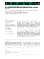
Figure 1: Overlap of Judgments of [10 minutes,
30 minutes] and [10 minutes, 2 hours].

In fact, what coders were instructed to anno-
tate for a given event is not just a range, but a
duration distribution for the event, where the
area between the lower bound and the upper
bound covers about 80% of the entire distribution

area. Since it’s natural to assume the most likely
duration for such distribution is its mean (aver-
age) duration, and the distribution flattens out
toward the upper and lower bounds, we use the
normal or Gaussian distribution to model our
duration distributions. If the area between lower
and upper bounds covers 80% of the entire dis-
tribution area, the bounds are each 1.28 standard
deviations from the mean.
Figure 1 shows the overlap in distributions for
judgments of [10 minutes, 30 minutes] and [10
minutes, 2 hours], and the overlap or agreement
is 0.508706.
2.2 Expected Agreement
What is the probability that the annotators agree
by chance for our task? The first quick response
to this question may be 0, if we consider all the
possible durations from 1 second to 1000 years
or even positive infinity.
However, not all the durations are equally pos-
sible. As in (Krippendorff, 1980), we assume
there exists one global distribution for our task
(i.e., the duration ranges for all the events), and
“chance” annotations would be consistent with
this distribution. Thus, the baseline will be an
annotator who knows the global distribution and
annotates in accordance with it, but does not read
the specific article being annotated. Therefore,
we must compute the global distribution of the
durations, in particular, of their means and their

widths. This will be of interest not only in deter-
mining expected agreement, but also in terms of
-5 0 5 10 15 20 25 30
0
20
40
60
80
100
120
140
160
180
Means of Annotated Durations
Number of Annotated Durations

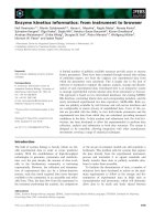
Figure 2: Distribution of Means of Annotated
Durations.

what it says about the genre of news articles and
about fuzzy judgments in general.
We first compute the distribution of the means
of all the annotated durations. Its histogram is
shown in Figure 2, where the horizontal axis
represents the mean values in the natural loga-
rithmic scale and the vertical axis represents the
number of annotated durations with that mean.
There are two peaks in this distribution. One is
from 5 to 7 in the natural logarithmic scale,
which corresponds to about 1.5 minutes to 30

minutes. The other is from 14 to 17 in the natural
logarithmic scale, which corresponds to about 8
days to 6 months. One could speculate that this
bimodal distribution is because daily newspapers
report short events that happened the day before
and place them in the context of larger trends.
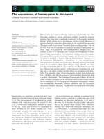
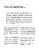
We also compute the distribution of the widths
(i.e., X
upper
– X
lower
) of all the annotated durations,
and its histogram is shown in Figure 3, where the
horizontal axis represents the width in the natural
logarithmic scale and the vertical axis represents
the number of annotated durations with that
width. Note that it peaks at about a half order of
magnitude (Hobbs and Kreinovich, 2001).
Since the global distribution is determined by
the above mean and width distributions, we can
then compute the expected agreement, i.e., the
probability that the annotators agree by chance,
where the chance is actually based on this global
distribution.
Two different methods were used to compute
the expected agreement (baseline), both yielding
nearly equal results. These are described in detail
in (Pan et al., 2006). For both, P(E) is about 0.15.

395

-5 0 5 10 15 20 25
0
50
100
150
200
250
300
350
400
Widths of Annotated Durations
N
um
b
er o
f

A
nno
t
a
t
e
d

D
ura
ti
ons

Figure 3: Distribution of Widths of Annotated
Durations.
3 Features
In this section, we describe the lexical, syntactic,
and semantic features that we considered in
learning event durations.
3.1 Local Context
For a given event, the local context features in-
clude a window of n tokens to its left and n to-
kens to its right, as well as the event itself, for n
= {0, 1, 2, 3}. The best n determined via cross
validation turned out to be 0, i.e., the event itself
with no local context. But we also present results
for n = 2 in Section 4.3 to evaluate the utility of
local context.
A token can be a word or a punctuation mark.
Punctuation marks are not removed, because they
can be indicative features for learning event du-
rations. For example, the quotation mark is a
good indication of quoted reporting events, and
the duration of such events most likely lasts for
seconds or minutes, depending on the length of
the quoted content. However, there are also cases
where quotation marks are used for other pur-
poses, such as emphasis of quoted words and
titles of artistic works.
For each token in the local context, including
the event itself, three features are included: the
original form of the token, its lemma (or root
form), and its part-of-speech (POS) tag. The

lemma of the token is extracted from parse trees
generated by the CONTEX parser (Hermjakob
and Mooney, 1997) which includes rich context
information in parse trees, and the Brill tagger
(Brill, 1992) is used for POS tagging.
The context window doesn’t cross the bounda-
ries of sentences. When there are not enough to-
kens on either side of the event within the win-
dow, “NULL” is used for the feature values.
Features Original Lemma POS
Event signed sign VBD
1token-after the the DT
2token-after plan plan NN
1token-before Friday Friday NNP
2token-before on on IN
Table 1: Local context features for the “signed”
event in sentence (1) with n = 2.

The local context features extracted for the
“signed” event in sentence (1) is shown in Table
1 (with a window size n = 2). The feature vector
is [signed, sign, VBD, the, the, DT, plan, plan,
NN, Friday, Friday, NNP, on, on, IN].

(1) The two presidents on Friday signed
the
plan.
3.2 Syntactic Relations
The information in the event’s syntactic envi-
ronment is very important in deciding the dura-

tions of events. For example, there is a difference
in the durations of the “watch” events in the
phrases “watch
a movie” and “watch a bird fly”.
For a given event, both the head of its subject
and the head of its object are extracted from the
parse trees generated by the CONTEX parser.
Similarly to the local context features, for both
the subject head and the object head, their origi-
nal form, lemma, and POS tags are extracted as
features. When there is no subject or object for
an event, “NULL” is used for the feature values.
For the “signed” event in sentence (1), the
head of its subject is “presidents” and the head of
its object is “plan”. The extracted syntactic rela-
tion features are shown in Table 2, and the fea-
ture vector is [presidents, president, NNS, plan,
plan, NN].
3.3 WordNet Hypernyms
Events with the same hypernyms may have simi-
lar durations. For example, events “ask” and
“talk” both have a direct WordNet (Miller, 1990)
hypernym of “communicate”, and most of the
time they do have very similar durations in the
corpus.
However, closely related events don’t always
have the same direct hypernyms. For example,
“see” has a direct hypernym of “perceive”,
whereas “observe” needs two steps up through
the hypernym hierarchy before reaching “per-

ceive”. Such correlation between events may be
lost if only the direct hypernyms of the words are
extracted.
396
Features Original Lemma POS
Subject presidents president NNS
Object plan plan NN
Table 2: Syntactic relation features for the
“signed” event in sentence (1).

Feature 1-hyper 2-hyper 3-hyper
Event write communicate interact
Subject
corporate
executive
executive
adminis-
trator
Object idea content cognition
Table 3: WordNet hypernym features for the
event (“signed”), its subject (“presidents”), and
its object (“plan”) in sentence (1).

It is useful to extract the hypernyms not only
for the event itself, but also for the subject and
object of the event. For example, events related
to a group of people or an organization usually
last longer than those involving individuals, and
the hypernyms can help distinguish such con-
cepts. For example, “society” has a “group” hy-

pernym (2 steps up in the hierarchy), and
“school” has an “organization” hypernym (3
steps up). The direct hypernyms of nouns are
always not general enough for such purpose, but
a hypernym at too high a level can be too general
to be useful. For our learning experiments, we
extract the first 3 levels of hypernyms from
WordNet.
Hypernyms are only extracted for the events
and their subjects and objects, not for the local
context words. For each level of hypernyms in
the hierarchy, it’s possible to have more than one
hypernym, for example, “see” has two direct hy-
pernyms, “perceive” and “comprehend”. For a
given word, it may also have more than one
sense in WordNet. In such cases, as in (Gildea
and Jurafsky, 2002), we only take the first sense
of the word and the first hypernym listed for each
level of the hierarchy. A word disambiguation
module might improve the learning performance.
But since the features we need are the hypernyms,
not the word sense itself, even if the first word
sense is not the correct one, its hypernyms can
still be good enough in many cases. For example,
in one news article, the word “controller” refers
to an air traffic controller, which corresponds to
the second sense in WordNet, but its first sense
(business controller) has the same hypernym of
“person” (3 levels up) as the second sense (direct
hypernym). Since we take the first 3 levels of

hypernyms, the correct hypernym is still ex-
tracted.

P(A) P(E) Kappa
0.528 0.740
0.877
0.500 0.755
Table 4: Inter-Annotator Agreement for Binary
Event Durations.

When there are less than 3 levels of hy-
pernyms for a given word, its hypernym on the
previous level is used. When there is no hy-
pernym for a given word (e.g., “go”), the word
itself will be used as its hypernyms. Since
WordNet only provides hypernyms for nouns
and verbs, “NULL” is used for the feature values
for a word that is not a noun or a verb.
For the “signed” event in sentence (1), the ex-
tracted WordNet hypernym features for the event
(“signed”), its subject (“presidents”), and its ob-
ject (“plan”) are shown in Table 3, and the fea-
ture vector is [write, communicate, interact, cor-
porate_executive, executive, administrator, idea,
content, cognition].
4 Experiments
The distribution of the means of the annotated
durations in Figure 2 is bimodal, dividing the
events into those that take less than a day and
those that take more than a day. Thus, in our first

machine learning experiment, we have tried to
learn this coarse-grained event duration informa-
tion as a binary classification task.
4.1 Inter-Annotator Agreement, Baseline,
and Upper Bound
Before evaluating the performance of different
learning algorithms, the inter-annotator agree-
ment, the baseline and the upper bound for the
learning task are assessed first.
Table 4 shows the inter-annotator agreement
results among 3 annotators for binary event dura-
tions. The experiments were conducted on the
same data sets as in (Pan et al., 2006). Two
kappa values are reported with different ways of
measuring expected agreement (P(E)), i.e.,
whether or not the annotators have prior knowl-
edge of the global distribution of the task.
The human agreement before reading the
guidelines (0.877) is a good estimate of the upper
bound performance for this binary classification
task. The baseline for the learning task is always
taking the most probable class. Since 59.0% of
the total data is “long” events, the baseline per-
formance is 59.0%.


397
Class Algor. Prec. Recall F-Score
SVM
0.707 0.606

0.653
NB 0.567 0.768 0.652
Short
C4.5 0.571 0.600 0.585
SVM
0.793 0.857
0.823
NB 0.834 0.665 0.740
Long

C4.5 0.765 0.743 0.754
Table 5: Test Performance of Three Algorithms.
4.2 Data
The original annotated data can be straightfor-
wardly transformed for this binary classification
task. For each event annotation, the most likely
(mean) duration is calculated first by averaging
(the logs of) its lower and upper bound durations.
If its most likely (mean) duration is less than a
day (about 11.4 in the natural logarithmic scale),
it is assigned to the “short” event class, otherwise
it is assigned to the “long” event class. (Note that
these labels are strictly a convenience and not an
analysis of the meanings of “short” and “long”.)
We divide the total annotated non-WSJ data
(2132 event instances) into two data sets: a train-
ing data set with 1705 event instances (about
80% of the total non-WSJ data) and a held-out
test data set with 427 event instances (about 20%
of the total non-WSJ data). The WSJ data (156

event instances) is kept for further test purposes
(see Section 4.4).
4.3 Experimental Results (non-WSJ)
Learning Algorithms. Three supervised learn-
ing algorithms were evaluated for our binary
classification task, namely, Support Vector Ma-
chines (SVM) (Vapnik, 1995), Naïve Bayes
(NB) (Duda and Hart, 1973), and Decision Trees
C4.5 (Quinlan, 1993). The Weka (Witten and
Frank, 2005) machine learning package was used
for the implementation of these learning algo-
rithms. Linear kernel is used for SVM in our ex-
periments.
Each event instance has a total of 18 feature
values, as described in Section 3, for the event
only condition, and 30 feature values for the lo-
cal context condition when n = 2. For SVM and
C4.5, all features are converted into binary fea-
tures (6665 and 12502 features).
Results. 10-fold cross validation was used to
train the learning models, which were then tested
on the unseen held-out test set, and the perform-
ance (including the precision, recall, and F-score
1


1 F-score is computed as the harmonic mean of the preci-
sion and recall: F = (2*Prec*Rec)/(Prec+Rec).
Algorithm Precision
Baseline 59.0%

C4.5 69.1%
NB 70.3%
SVM 76.6%
Human Agreement 87.7%
Table 6: Overall Test Precision on non-WSJ
Data.

for each class) of the three learning algorithms is
shown in Table 5. The significant measure is
overall precision, and this is shown for the three
algorithms in Table 6, together with human a-
greement (the upper bound of the learning task)
and the baseline.
We can see that among all three learning algo-
rithms, SVM achieves the best F-score for each
class and also the best overall precision (76.6%).
Compared with the baseline (59.0%) and human
agreement (87.7%), this level of performance is
very encouraging, especially as the learning is
from such limited training data.
Feature Evaluation. The best performing
learning algorithm, SVM, was then used to ex-
amine the utility of combinations of four differ-
ent feature sets (i.e., event, local context, syntac-
tic, and WordNet hypernym features). The de-
tailed comparison is shown in Table 7.
We can see that most of the performance
comes from event word or phrase itself. A sig-
nificant improvement above that is due to the
addition of information about the subject and

object. Local context does not help and in fact
may hurt, and hypernym information also does
not seem to help
2
. It is of interest that the most
important information is that from the predicate
and arguments describing the event, as our lin-
guistic intuitions would lead us to expect.
4.4 Test on WSJ Data
Section 4.3 shows the experimental results with
the learned model trained and tested on the data
with the same genre, i.e., non-WSJ articles.
In order to evaluate whether the learned model
can perform well on data from different news
genres, we tested it on the unseen WSJ data (156
event instances). The performance (including the
precision, recall, and F-score for each class) is
shown in Table 8. The precision (75.0%) is very
close to the test performance on the non-WSJ

2 In the “Syn+Hyper” cases, the learning algorithm with and
without local context gives identical results, probably be-
cause the other features dominate.
398
Event Only (n = 0) Event Only + Syntactic Event + Syn + Hyper
Class
Prec. Rec. F Prec. Rec. F Prec. Rec. F
Short 0.742 0.465 0.571 0.758 0.587 0.662 0.707 0.606 0.653
Long 0.748 0.908 0.821 0.792 0.893 0.839 0.793 0.857 0.823
Overall Prec.

74.7% 78.2% 76.6%

Local Context (n = 2) Context + Syntactic Context + Syn + Hyper
Short 0.672 0.568 0.615 0.710 0.600 0.650 0.707 0.606 0.653
Long 0.774 0.842 0.806 0.791 0.860 0.824 0.793 0.857 0.823
Overall Prec.
74.2% 76.6% 76.6%
Table 7: Feature Evaluation with Different Feature Sets using SVM.

Class Prec. Rec. F
Short 0.692 0.610 0.649
Long 0.779 0.835 0.806
Overall Prec.
75.0%
Table 8: Test Performance on WSJ data.

P(A) P(E) Kappa
0.151 0.762
0.798
0.143 0.764
Table 9: Inter-Annotator Agreement for Most
Likely Temporal Unit.

data, and indicates the significant generalization
capacity of the learned model.
5 Learning the Most Likely Temporal
Unit
These encouraging results have prompted us to
try to learn more fine-grained event duration in-
formation, viz., the most likely temporal units of

event durations (cf. (Rieger 1974)’s
ORDER-
HOURS
, ORDERDAYS).
For each original event annotation, we can ob-
tain the most likely (mean) duration by averaging
its lower and upper bound durations, and assign-
ing it to one of seven classes (i.e., second, min-
ute, hour, day, week, month, and year) based on
the temporal unit of its most likely duration.
However, human agreement on this more fine-
grained task is low (44.4%). Based on this obser-
vation, instead of evaluating the exact agreement
between annotators, an “approximate agreement”
is computed for the most likely temporal unit of
events. In “approximate agreement”, temporal
units are considered to match if they are the same
temporal unit or an adjacent one. For example,
“second” and “minute” match, but “minute” and
“day” do not.
Some preliminary experiments have been con-
ducted for learning this multi-classification task.
The same data sets as in the binary classification
task were used. The only difference is that the
class for each instance is now labeled with one
Algorithm Precision
Baseline 51.5%
C4.5 56.4%
NB 65.8%
SVM 67.9%

Human Agreement 79.8%
Table 10: Overall Test Precisions.

of the seven temporal unit classes.
The baseline for this multi-classification task
is always taking the temporal unit which with its
two neighbors spans the greatest amount of data.
Since the “week”, “month”, and “year” classes
together take up largest portion (51.5%) of the
data, the baseline is always taking the “month”
class, where both “week” and “year” are also
considered a match. Table 9 shows the inter-
annotator agreement results for most likely tem-
poral unit when using “approximate agreement”.
Human agreement (the upper bound) for this
learning task increases from 44.4% to 79.8%.
10-fold cross validation was also used to train
the learning models, which were then tested on
the unseen held-out test set. The performance of
the three algorithms is shown in Table 10. The
best performing learning algorithm is again SVM
with 67.9% test precision. Compared with the
baseline (51.5%) and human agreement (79.8%),
this again is a very promising result, especially
for a multi-classification task with such limited
training data. It is reasonable to expect that when
more annotated data becomes available, the
learning algorithm will achieve higher perform-
ance when learning this and more fine-grained
event duration information.

Although the coarse-grained duration informa-
tion may look too coarse to be useful, computers
have no idea at all whether a meeting event takes
seconds or centuries, so even coarse-grained es-
timates would give it a useful rough sense of how
long each event may take. More fine-grained du-
ration information is definitely more desirable
for temporal reasoning tasks. But coarse-grained
399
durations to a level of temporal units can already
be very useful.
6 Conclusion
In the research described in this paper, we have
addressed a problem extracting information
about event durations encoded in event descrip-
tions that has heretofore received very little
attention in the field. It is information that can
have a substantial impact on applications where
the temporal placement of events is important.
Moreover, it is representative of a set of prob-
lems – making use of the vague information in
text – that has largely eluded empirical ap-
proaches in the past. In (Pan et al., 2006), we
explicate the linguistic categories of the phenom-
ena that give rise to grossly discrepant judgments
among annotators, and give guidelines on resolv-
ing these discrepancies. In the present paper, we
describe a method for measuring inter-annotator
agreement when the judgments are intervals on a
scale; this should extend from time to other sca-

lar judgments. Inter-annotator agreement is too
low on fine-grained judgments. However, for the
coarse-grained judgments of more than or less
than a day, and of approximate agreement on
temporal unit, human agreement is acceptably
high. For these cases, we have shown that ma-
chine-learning techniques achieve impressive
results.
Acknowledgments
This work was supported by the Advanced Re-
search and Development Activity (ARDA), now
the Disruptive Technology Office (DTO), under
DOD/DOI/ARDA Contract No. NBCHC040027.
The authors have profited from discussions with
Hoa Trang Dang, Donghui Feng, Kevin Knight,
Daniel Marcu, James Pustejovsky, Deepak Ravi-
chandran, and Nathan Sobo.
References
B. Boguraev and R. K. Ando. 2005. TimeML-
Compliant Text Analysis for Temporal Reasoning.
In Proceedings of International Joint Conference
on Artificial Intelligence (IJCAI).
E. Brill. 1992. A simple rule-based part of speech
tagger. In Proceedings of the Third Conference on
Applied Natural Language Processing.
J. Carletta. 1996. Assessing agreement on classifica-
tion tasks: the kappa statistic. Computational Lin-
gustics, 22(2):249–254.
R. O. Duda and P. E. Hart. 1973. Pattern Classifica-
tion and Scene Analysis. Wiley, New York.

E. Filatova and E. Hovy. 2001. Assigning Time-
Stamps to Event-Clauses. Proceedings of ACL
Workshop on Temporal and Spatial Reasoning.
P. Fortemps. 1997. Jobshop Scheduling with Impre-
cise Durations: A Fuzzy Approach. IEEE Transac-
tions on Fuzzy Systems Vol. 5 No. 4.
D. Gildea and D. Jurafsky. 2002. Automatic Labeling
of Semantic Roles. Computational Linguistics,
28(3):245-288.
L. Godo and L. Vila. 1995. Possibilistic Temporal
Reasoning based on Fuzzy Temporal Constraints.
In Proceedings of International Joint Conference
on Artificial Intelligence (IJCAI).
U. Hermjakob and R. J. Mooney. 1997. Learning
Parse and Translation Decisions from Examples
with Rich Context. In Proceedings of the 35th An-
nual Meeting of the Association for Computational
Linguistics (ACL).
J. Hitzeman, M. Moens, and C. Grover. 1995. Algo-
rithms for Analyzing the Temporal Structure of
Discourse. In Proceedings of EACL. Dublin, Ire-
land.
J. R. Hobbs and V. Kreinovich. 2001. Optimal Choice
of Granularity in Commonsense Estimation: Why
Half Orders of Magnitude, In Proceedings of Joint
9th IFSA World Congress and 20th NAFIPS Inter-
national Conference, Vacouver, British Columbia.
K. Krippendorf. 1980. Content Analysis: An introduc-
tion to its methodology. Sage Publications.
I. Mani and G. Wilson. 2000. Robust Temporal Proc-

essing of News. In Proceedings of the 38th Annual
Meeting of the Association for Computational Lin-
guistics (ACL).
G. A. Miller. 1990. WordNet: an On-line Lexical Da-
tabase. International Journal of Lexicography 3(4).
F. Pan, R. Mulkar, and J. R. Hobbs. 2006. An Anno-
tated Corpus of Typical Durations of Events. In
Proceedings of the Fifth International Conference
on Language Resources and Evaluation (LREC),
Genoa, Italy.
J. Pustejovsky, P. Hanks, R. Saurí, A. See, R. Gai-
zauskas, A. Setzer, D. Radev, B. Sundheim, D.
Day, L. Ferro and M. Lazo. 2003. The timebank
corpus. In Corpus Linguistics, Lancaster, U.K.
J. R. Quinlan. 1993. C4.5: Programs for Machine
Learning. Morgan Kaufmann, San Francisco.
C. J. Rieger. 1974. Conceptual memory: A theory and
computer program for processing and meaning
content of natural language utterances. Stanford
AIM-233.
V. Vapnik. 1995. The Nature of Statistical Learning
Theory. Springer-Verlag, New York.
I. H. Witten and E. Frank. 2005. Data Mining: Practi-
cal machine learning tools and techniques, 2nd
Edition, Morgan Kaufmann, San Francisco.
400