Tài liệu Báo cáo khoa học: "Learning Accurate, Compact, and Interpretable Tree Annotation" ppt

Proceedings of the 21st International Conference on Computational Linguistics and 44th Annual Meeting of the ACL, pages 433–440,
Sydney, July 2006.
c
2006 Association for Computational Linguistics
Learning Accurate, Compact, and Interpretable Tree Annotation
Slav Petrov Leon Barrett Romain Thibaux Dan Klein
Computer Science Division, EECS Department
University of California at Berkeley
Berkeley, CA 94720
{petrov, lbarrett, thibaux, klein}@eecs.berkeley.edu
Abstract
We present an automatic approach to tree annota-
tion in which basic nonterminal symbols are alter-
nately split and merged to maximize the likelihood
of a training treebank. Starting with a simple X-
bar grammar, we learn a new grammar whose non-
terminals are subsymbols of the original nontermi-
nals. In contrast with previous work, we are able
to split various terminals to different degrees, as ap-
propriate to the actual complexity in the data. Our
grammars automatically learn the kinds of linguistic
distinctions exhibited in previous work on manual
tree annotation. On the other hand, our grammars
are much more compact and substantially more ac-
curate than previous work on automatic annotation.
Despite its simplicity, our best grammar achieves
an F
1
of 90.2% on the Penn Treebank, higher than
fully lexicalized systems.
1 Introduction

Probabilistic context-free grammars (PCFGs) underlie
most high-performance parsers in one way or another
(Collins, 1999; Charniak, 2000; Charniak and Johnson,
2005). However, as demonstrated in Charniak (1996)
and Klein and Manning (2003), a PCFG which sim-
ply takes the empirical rules and probabilities off of a
treebank does not perform well. This naive grammar
is a poor one because its context-freedom assumptions
are too strong in some places (e.g. it assumes that sub-
ject and object NPs share the same distribution) and too
weak in others (e.g. it assumes that long rewrites are
not decomposable into smaller steps). Therefore, a va-
riety of techniques have been developed to both enrich
and generalize the naive grammar, ranging from simple
tree annotation and symbol splitting (Johnson, 1998;
Klein and Manning, 2003) to full lexicalization and in-
tricate smoothing (Collins, 1999; Charniak, 2000).
In this paper, we investigate the learning of a gram-
mar consistent with a treebank at the level of evalua-
tion symbols (such as NP, VP, etc.) but split based on
the likelihood of the training trees. Klein and Manning
(2003) addressed this question from a linguistic per-
spective, starting with a Markov grammar and manu-
ally splitting symbols in response to observed linguistic
trends in the data. For example, the symbol NP might
be split into the subsymbol NPˆS in subject position
and the subsymbol NPˆVP in object position. Recently,
Matsuzaki et al. (2005) and also Prescher (2005) ex-
hibited an automatic approach in which each symbol is
split into a fixed number of subsymbols. For example,

NP would be split into NP-1 through NP-8. Their ex-
citing result was that, while grammars quickly grewtoo
large to be managed, a 16-subsymbol induced grammar
reached the parsing performance of Klein and Manning
(2003)’s manual grammar. Other work has also investi-
gated aspects of automatic grammar refinement; for ex-
ample, Chiang and Bikel (2002) learn annotations such
as head rules in a constrained declarative language for
tree-adjoining grammars.
We present a method that combines the strengths of
both manual and automatic approaches while address-
ing some of their common shortcomings. Like Mat-
suzaki et al. (2005) and Prescher (2005), we induce
splits in a fully automatic fashion. However, we use a
more sophisticated split-and-merge approach that allo-
cates subsymbols adaptivelywhere they are most effec-
tive, like a linguist would. The grammars recover pat-
terns like those discussed in Klein and Manning (2003),
heavily articulating complex and frequent categories
like NP and VP while barely splitting rare or simple
ones (see Section 3 for an empirical analysis).
Empirically, hierarchical splitting increases the ac-
curacy and lowers the variance of the learned gram-
mars. Another contribution is that, unlike previous
work, we investigate smoothed models, allowing us to
split grammars more heavily before running into the
oversplitting effect discussed in Klein and Manning
(2003), where data fragmentation outweighs increased
expressivity.
Our method is capable of learning grammars of sub-

stantially smaller size and higher accuracy than previ-
ous grammar refinement work, starting from a simpler
initial grammar. For example, even beginning with an
X-bar grammar (see Section 1.1) with 98 symbols, our
best grammar, using 1043 symbols, achieves a test set
F
1
of 90.2%. This is a 27% reduction in error and a sig-
nificant reduction in size
1
over the most accurate gram-
1
This is a 97.5% reduction in number of symbols. Mat-
suzaki et al. (2005) do not report a number of rules, but our
small number of symbols and our hierarchical training (which
433
(a) FRAG
RB
Not
NP
DT
this
NN
year
.
.
(b) ROOT
FRAG
FRAG
RB

Not
NP
DT
this
NN
year
.
.
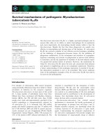
Figure 1: (a) The original tree. (b) The X-bar tree.
mar in Matsuzaki et al. (2005). Our grammar’s accu-
racy was higher than fully lexicalized systems, includ-
ing the maximum-entropy inspired parser of Charniak
and Johnson (2005).
1.1 Experimental Setup
We ran our experiments on the Wall Street Journal
(WSJ) portion of the Penn Treebank using the stan-
dard setup: we trained on sections 2 to 21, and we
used section 1 as a validation set for tuning model hy-
perparameters. Section 22 was used as development
set for intermediate results. All of section 23 was re-
served for the final test. We used the EVALB parseval
reference implementation, available from Sekine and
Collins (1997), for scoring. All reported development
set results are averages over four runs. For the final test
we selected the grammar that performed best on the de-
velopment set.
Our experiments are based on a completely unanno-
tated X-bar style grammar, obtained directly from the
Penn Treebank by the binarization procedure shown in
Figure 1. For each local tree rooted at an evaluation

nonterminal X, we introduce a cascade of new nodes
labeled X so that each has two children. Rather than
experiment with head-outward binarization as in Klein
and Manning (2003), we simply used a left branching
binarization; Matsuzaki et al. (2005) contains a com-
parison showing that the differences between binariza-
tions are small.
2 Learning
To obtain a grammar from the training trees, we want
to learn a set of rule probabilities β on latent annota-
tions that maximize the likelihood of the training trees,
despite the fact that the original trees lack the latent
annotations. The Expectation-Maximization (EM) al-
gorithm allows us to do exactly that.
2
Given a sen-
tence w and its unannotated tree T , consider a non-
terminal A spanning (r, t) and its children B and C
spanning (r, s) and (s, t). Let A
x
be a subsymbol
of A, B
y
of B, and C
z
of C. Then the inside and
outside probabilities P
IN
(r, t, A
x

)
def
= P (w
r:t
|A
x
) and
P
OUT
(r, t, A
x
)
def
= P (w
1:r
A
x
w
t:n
) can be computed re-
encourages sparsity) suggest a large reduction.
2
Other techniques are also possible; Henderson (2004)
uses neural networks to induce latent left-corner parser states.
cursively:
P
IN
(r, t, A
x
) =


y,z
β(A
x
→ B
y
C
z
)
×P
IN
(r, s, B
y
)P
IN
(s, t, C
z
)
P
OUT
(r, s, B
y
) =

x,z
β(A
x
→ B
y
C

z
)
×P
OUT
(r, t, A
x
)P
IN
(s, t, C
z
)
P
OUT
(s, t, C
z
) =

x,y
β(A
x
→ B
y
C
z
)
×P
OUT
(r, t, A
x
)P

IN
(r, s, B
y
)
Although we show only the binary component here, of
course there are both binary and unary productions that
are included. In the Expectation step, one computes
the posterior probability of each annotated rule and po-
sition in each training set tree T :
P ((r, s, t, A
x
→ B
y
C
z
)|w, T ) ∝ P
OUT
(r, t, A
x
)
×β(A
x
→ B
y
C
z
)P
IN
(r, s, B
y

)P
IN
(s, t, C
z
) (1)
In the Maximization step, one uses the above probabil-
ities as weighted observations to update the rule proba-
bilities:
β(A
x
→ B
y
C
z
) :=
#{A
x
→ B
y
C
z
}

y
′
,z
′
#{A
x
→ B

y
′
C
z
′
}
Note that, because there is no uncertainty about the lo-
cation of the brackets, this formulation of the inside-
outside algorithm is linear in the length of the sentence
rather than cubic (Pereira and Schabes, 1992).
For our lexicon, we used a simple yet robust method
for dealing with unknown and rare words by extract-
ing a small number of features from the word and then
computing appproximate tagging probabilities.
3
2.1 Initialization
EM is only guaranteed to find a local maximum of the
likelihood, and, indeed, in practice it often gets stuck in
a suboptimal configuration. If the search space is very
large, even restarting may not be sufficient to alleviate
this problem. One workaround is to manually specify
some of the annotations. For instance, Matsuzaki et al.
(2005) start by annotating their grammar with the iden-
tity of the parent and sibling, which are observed (i.e.
not latent), before adding latent annotations.
4
If these
manual annotations are good, they reduce the search
space for EM by constraining it to a smaller region. On
the other hand, this pre-splitting defeats some of the

purpose of automatically learning latent annotations,
3
A word is classified into one of 50 unknown word cate-
gories based on the presence of features such as capital let-
ters, digits, and certain suffixes and its tagging probability is
given by: P
′
(word|tag) = k
ˆ
P(class|tag) where k is a con-
stant representing P (word|class) and can simply be dropped.
Rare words are modeled using a combination of their known
and unknown distributions.
4
In other words, in the terminology of Klein and Man-
ning (2003), they begin with a (vertical order=2, horizontal
order=1) baseline grammar.
434
DT
the (0.50) a (0.24) The (0.08)
that (0.15) this (0.14) some (0.11)
this (0.39)
that (0.28)
That (0.11)
this (0.52)
that (0.36)
another (0.04)
That (0.38)
This (0.34)
each (0.07)

some (0.20)
all (0.19)
those (0.12)
some (0.37)
all (0.29)
those (0.14)
these (0.27)
both (0.21)
Some (0.15)
the (0.54) a (0.25) The (0.09)
the (0.80)
The (0.15)
a (0.01)
the (0.96)
a (0.01)
The (0.01)
The (0.93)
A(0.02)
No(0.01)
a (0.61)
the (0.19)
an (0.10)
a (0.75)
an (0.12)
the (0.03)
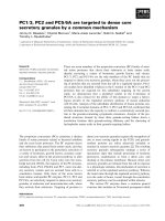
Figure 2: Evolution of the DT tag during hierarchical splitting and merging. Shown are the top three words for
each subcategory and their respective probability.
leaving to the user the task of guessing what a good
starting annotation might be.
We take a different, fully automated approach. We

start with a completely unannotated X-bar style gram-
mar as described in Section 1.1. Since we will evaluate
our grammar on its ability to recoverthe Penn Treebank
nonterminals, we must include them in our grammar.
Therefore, this initialization is the absolute minimum
starting grammar that includes the evaluation nontermi-
nals (and maintains separate grammar symbols for each
of them).
5
It is a very compact grammar: 98 symbols,
6
236 unary rules, and 3840 binary rules. However, it
also has a very low parsing performance: 65.8/59.8
LP/LR on the development set.
2.2 Splitting
Beginning with this baseline grammar, we repeatedly
split and re-train the grammar. In each iteration we
initialize EM with the results of the smaller gram-
mar, splitting every previous annotation symbol in two
and adding a small amount of randomness (1%) to
break the symmetry. The results are shown in Fig-
ure 3. Hierarchical splitting leads to better parame-
ter estimates over directly estimating a grammar with
2
k
subsymbols per symbol. While the two procedures
are identical for only two subsymbols (F
1
: 76.1%),
the hierarchical training performs better for four sub-

symbols (83.7% vs. 83.2%). This advantage grows
as the number of subsymbols increases (88.4% vs.
87.3% for 16 subsymbols). This trend is to be ex-
pected, as the possible interactions between the sub-
symbols grows as their number grows. As an exam-
ple of how staged training proceeds, Figure 2 shows
the evolution of the subsymbols of the determiner (DT)
tag, which first splits demonstratives from determiners,
then splits quantificational elements from demonstra-
tives along one branch and definites from indefinites
along the other.
5
If our purpose was only to model language, as measured
for instance by perplexity on new text, it could make sense
to erase even the labels of the Penn Treebank to let EM find
better labels by itself, giving an experiment similar to that of
Pereira and Schabes (1992).
6
45 part of speech tags, 27 phrasal categories and the 26
intermediate symbols which were added during binarization
Because EM is a local search method, it is likely to
converge to different local maxima for different runs.
In our case, the variance is higher for models with few
subcategories; because not all dependencies can be ex-
pressed with the limited number of subcategories, the
results vary depending on which one EM selects first.
As the grammar size increases, the important depen-
dencies can be modeled, so the variance decreases.
2.3 Merging
It is clear from all previous work that creating more la-

tent annotations can increase accuracy. On the other
hand, oversplitting the grammar can be a serious prob-
lem, as detailed in Klein and Manning (2003). Adding
subsymbols divides grammar statistics into many bins,
resulting in a tighter fit to the training data. At the same
time, each bin gives a less robust estimate of the gram-
mar probabilities, leading to overfitting. Therefore, it
would be to our advantage to split the latent annota-
tions only where needed, rather than splitting them all
as in Matsuzaki et al. (2005). In addition, if all sym-
bols are split equally often, one quickly (4 split cycles)
reaches the limits of what is computationally feasible
in terms of training time and memory usage.
Consider the comma POS tag. We would like to see
only one sort of this tag because, despite its frequency,
it always produces the terminal comma (barring a few
annotation errors in the treebank). On the other hand,
we would expect to find an advantage in distinguishing
between various verbal categories and NP types. Addi-
tionally, splitting symbols like the comma is not only
unnecessary, but potentially harmful, since it need-
lessly fragments observations of other symbols’ behav-
ior.
It should be noted that simple frequency statistics are
not sufficient for determining how often to split each
symbol. Consider the closed part-of-speech classes
(e.g. DT, CC, IN) or the nonterminal ADJP. These
symbols are very common, and certainly do contain
subcategories, but there is little to be gained from
exhaustively splitting them before even beginning to

model the rarer symbols that describe the complex in-
ner correlations inside verb phrases. Our solution is
to use a split-and-merge approach broadly reminiscent
of ISODATA, a classic clustering procedure (Ball and
435
Hall, 1967).
To prevent oversplitting, we could measure the util-
ity of splitting each latent annotation individually and
then split the best ones first. However, not only is this
impractical, requiring an entire training phase for each
new split, but it assumes the contributions of multiple
splits are independent. In fact, extra subsymbols may
need to be added to several nonterminals before they
can cooperate to pass information along the parse tree.
Therefore, we go in the opposite direction; that is, we
split every symbol in two, train, and then measure for
each annotation the loss in likelihood incurred when
removing it. If this loss is small, the new annotation
does not carry enough useful information and can be
removed. What is more, contrary to the gain in like-
lihood for splitting, the loss in likelihood for merging
can be efficiently approximated.
7
Let T be a training tree generating a sentence w.
Consider a node n of T spanning (r, t) with the label
A; that is, the subtree rooted at n generates w
r:t
and
has the label A. In the latent model, its label A is split
up into several latent labels, A

x
. The likelihood of the
data can be recovered from the inside and outside prob-
abilities at n:
P(w, T ) =

x
P
IN
(r, t, A
x
)P
OUT
(r, t, A
x
) (2)
Consider merging, at n only, two annotations A
1
and
A
2
. Since A now combines the statistics of A
1
and A
2
,
its production probabilities are the sum of those of A
1
and A
2

, weighted by their relative frequency p
1
and p
2
in the training data. Therefore the inside score of A is:
P
IN
(r, t, A) = p
1
P
IN
(r, t, A
1
) + p
2
P
IN
(r, t, A
2
)
Since A can be produced as A
1
or A
2
by its parents, its
outside score is:
P
OUT
(r, t, A) = P
OUT

(r, t, A
1
) + P
OUT
(r, t, A
2
)
Replacing these quantities in (2) gives us the likelihood
P
n
(w, T ) where these two annotations and their corre-
sponding rules have been merged, around only node n.
We approximate the overall loss in data likelihood
due to merging A
1
and A
2
everywhere in all sentences
w
i
by the product of this loss for each local change:
∆
ANNOTATION
(A
1
, A
2
) =

i


n∈T
i
P
n
(w
i
, T
i
)
P(w
i
, T
i
)
This expression is an approximation because it neglects
interactions between instances of a symbol at multiple
places in the same tree. These instances, however, are
7
The idea of merging complex hypotheses to encourage
generalization is also examined in Stolcke and Omohundro
(1994), who used a chunking approach to propose new pro-
ductions in fully unsupervised grammar induction. They also
found it necessary to make local choices to guide their likeli-
hood search.
often far apart and are likely to interact only weakly,
and this simplification avoids the prohibitive cost of
running an inference algorithm for each tree and an-
notation. We refer to the operation of splitting anno-
tations and re-merging some them based on likelihood

loss as a split-merge (SM) cycle. SM cycles allow us to
progressively increase the complexity of our grammar,
giving priority to the most useful extensions.
In our experiments, merging was quite valuable. De-
pending on how many splits were reversed, we could
reduce the grammar size at the cost of little or no loss
of performance, or even a gain. We found that merging
50% of the newly split symbols dramatically reduced
the grammar size after each splitting round, so that af-
ter 6 SM cycles, the grammar was only 17% of the size
it would otherwise have been (1043 vs. 6273 subcat-
egories), while at the same time there was no loss in
accuracy (Figure 3). Actually, the accuracy even in-
creases, by 1.1% at 5 SM cycles. The numbers of splits
learned turned out to not be a direct function of symbol
frequency; the numbers of symbols for both lexical and
nonlexical tags after 4 SM cycles are given in Table 2.
Furthermore, merging makes large amounts of splitting
possible. It allows us to go from 4 splits, equivalent to
the 2
4
= 16 substates of Matsuzaki et al. (2005), to 6
SM iterations, which take a few days to run on the Penn
Treebank.
2.4 Smoothing
Splitting nonterminals leads to a better fit to the data by
allowing each annotation to specialize in representing
only a fraction of the data. The smaller this fraction,
the higher the risk of overfitting. Merging, by allow-
ing only the most beneficial annotations, helps mitigate

this risk, but it is not the only way. We can further
minimize overfitting by forcing the production proba-
bilities from annotations of the same nonterminal to be
similar. For example, a noun phrase in subject position
certainly has a distinct distribution, but it may benefit
from being smoothed with counts from all other noun
phrases. Smoothing the productions of each subsym-
bol by shrinking them towards their common base sym-
bol gives us a more reliable estimate, allowing them to
share statistical strength.
We perform smoothing in a linear way. The es-
timated probability of a production p
x
= P(A
x
→
B
y
C
z
) is interpolated with the average over all sub-
symbols of A.
p
′
x
= (1 − α)p
x
+ α¯p where ¯p =
1
n


x
p
x
Here, α is a small constant: we found 0.01 to be a good
value, but the actual quantity was surprisingly unimpor-
tant. Because smoothing is most necessary when pro-
duction statistics are least reliable, we expect smooth-
ing to help more with larger numbers of subsymbols.
This is exactly what we observe in Figure 3, where
smoothing initially hurts (subsymbols are quite distinct
436
and do not need their estimates pooled) but eventually
helps (as symbols have finer distinctions in behavior
and smaller data support).
2.5 Parsing
When parsing new sentences with an annotated gram-
mar, returning the most likely (unannotated) tree is in-
tractable: to obtain the probability of an unannotated
tree, one must sum over combinatorially many annota-
tion trees (derivations) for each tree (Sima’an, 1992).
Matsuzaki et al. (2005) discuss two approximations.
The first is settling for the most probable derivation
rather than most probableparse, i.e. returning the single
most likely (Viterbi) annotated tree (derivation). This
approximation is justified if the sum is dominated by
one particular annotated tree. The second approxima-
tion that Matsuzaki et al. (2005) present is the Viterbi
parse under a new sentence-specific PCFG, whose rule
probabilities are given as the solution of a variational

approximation of the original grammar. However, their
rule probabilities turn out to be the posterior probabil-
ity, given the sentence, of each rule being used at each
position in the tree. Their algorithm is therefore the la-
belled recall algorithm of Goodman (1996) but applied
to rules. That is, it returns the tree whose expected
number of correct rules is maximal. Thus, assuming
one is interested in a per-position score like F
1
(which
is its own debate), this method of parsing is actually
more appropriate than finding the most likely parse,
not simply a cheap approximation of it, and it need not
be derived by a variational argument. We refer to this
method of parsing as the max-rule parser. Since this
method is not a contribution of this paper, we refer the
reader to the fuller presentations in Goodman (1996)
and Matsuzaki et al. (2005). Note that contrary to the
original labelled recall algorithm, which maximizes the
number of correct symbols, this tree only contains rules
allowed by the grammar. As a result, the percentage of
complete matches with the max-rule parser is typically
higher than with the Viterbi parser. (37.5% vs. 35.8%
for our best grammar).
These posterior rule probabilities are still given by
(1), but, since the structure of the tree is no longer
known, we must sum over it when computing the in-
side and outside probabilities:
P
IN

(r, t, A
x
) =

B,C,s

y,z
β(A
x
→ B
y
C
z
)×
P
IN
(r, s, B
y
)P
IN
(s, t, C
z
)
P
OUT
(r, s, B
y
) =

A,C,t


x,z
β(A
x
→ B
y
C
z
)×
P
OUT
(r, t, A
x
)P
IN
(s, t, C
z
)
P
OUT
(s, t, C
z
) =

A,B,r

x,y
β(A
x
→ B

y
C
z
)×
P
OUT
(r, t, A
x
)P
IN
(r, s, B
y
)
For efficiency reasons, we use a coarse-to-fine prun-
ing scheme like that of Caraballo and Charniak (1998).
For a given sentence, we first run the inside-outside
algorithm using the baseline (unannotated) grammar,
74
76
78
80
82
84
86
88
90
200 400 600 800 1000
F1
Total number of grammar symbols
50% Merging and Smoothing

50% Merging
Splitting but no Merging
Flat Training
Figure 3: Hierarchical training leads to better parame-
ter estimates. Merging reduces the grammar size sig-
nificantly, while preserving the accuracy and enabling
us to do more SM cycles. Parameter smoothing leads
to even better accuracy for grammars with high com-
plexity.
producing a packed forest representation of the poste-
rior symbol probabilities for each span. For example,
one span might have a posterior probability of 0.8 of
the symbol NP, but e
−10
for PP. Then, we parse with the
larger annotated grammar, but, at each span, we prune
away any symbols whose posterior probability under
the baseline grammar falls below a certain threshold
(e
−8
in our experiments). Even though our baseline
grammar has a very low accuracy, we found that this
pruning barely impacts the performance of our better
grammars, while significantly reducing the computa-
tional cost. For a grammar with 479 subcategories (4
SM cycles), lowering the threshold to e
−15
led to an F
1
improvement of 0.13% (89.03 vs. 89.16) on the devel-

opment set but increased the parsing time by a factor of
16.
3 Analysis
So far, we have presented a split-merge method for
learning to iteratively subcategorize basic symbols
like NP and VP into automatically induced subsym-
bols (subcategories in the original sense of Chomsky
(1965)). This approach gives parsing accuracies of up
to 90.7% on the development set, substantially higher
than previous symbol-splitting approaches, while start-
ing from an extremely simple base grammar. However,
in general, any automatic induction system is in dan-
ger of being entirely uninterpretable. In this section,
we examine the learned grammars, discussing what is
learned. We focus particularly on connections with the
linguistically motivated annotations of Klein and Man-
ning (2003), which we do generally recover.
Inspecting a large grammar by hand is difficult, but
fortunately, our baseline grammar has less than 100
nonterminal symbols, and even our most complicated
grammar has only 1043 total (sub)symbols. It is there-
437
VBZ
VBZ-0 gives sells takes
VBZ-1 comes goes works
VBZ-2 includes owns is
VBZ-3 puts provides takes
VBZ-4 says adds Says
VBZ-5 believes means thinks
VBZ-6 expects makes calls

VBZ-7 plans expects wants
VBZ-8 is ’s gets
VBZ-9 ’s is remains
VBZ-10 has ’s is
VBZ-11 does Is Does
NNP
NNP-0 Jr. Goldman INC.
NNP-1 Bush Noriega Peters
NNP-2 J. E. L.
NNP-3 York Francisco Street
NNP-4 Inc Exchange Co
NNP-5 Inc. Corp. Co.
NNP-6 Stock Exchange York
NNP-7 Corp. Inc. Group
NNP-8 Congress Japan IBM
NNP-9 Friday September August
NNP-10 Shearson D. Ford
NNP-11 U.S. Treasury Senate
NNP-12 John Robert James
NNP-13 Mr. Ms. President
NNP-14 Oct. Nov. Sept.
NNP-15 New San Wall
JJS
JJS-0 largest latest biggest
JJS-1 least best worst
JJS-2 most Most least
DT
DT-0 the The a
DT-1 A An Another
DT-2 The No This

DT-3 The Some These
DT-4 all those some
DT-5 some these both
DT-6 That This each
DT-7 this that each
DT-8 the The a
DT-9 no any some
DT-10 an a the
DT-11 a this the
CD
CD-0 1 50 100
CD-1 8.50 15 1.2
CD-2 8 10 20
CD-3 1 30 31
CD-4 1989 1990 1988
CD-5 1988 1987 1990
CD-6 two three five
CD-7 one One Three
CD-8 12 34 14
CD-9 78 58 34
CD-10 one two three
CD-11 million billion trillion
PRP
PRP-0 It He I
PRP-1 it he they
PRP-2 it them him
RBR
RBR-0 further lower higher
RBR-1 more less More
RBR-2 earlier Earlier later

IN
IN-0 In With After
IN-1 In For At
IN-2 in for on
IN-3 of for on
IN-4 from on with
IN-5 at for by
IN-6 by in with
IN-7 for with on
IN-8 If While As
IN-9 because if while
IN-10 whether if That
IN-11 that like whether
IN-12 about over between
IN-13 as de Up
IN-14 than ago until
IN-15 out up down
RB
RB-0 recently previously still
RB-1 here back now
RB-2 very highly relatively
RB-3 so too as
RB-4 also now still
RB-5 however Now However
RB-6 much far enough
RB-7 even well then
RB-8 as about nearly
RB-9 only just almost
RB-10 ago earlier later
RB-11 rather instead because

RB-12 back close ahead
RB-13 up down off
RB-14 not Not maybe
RB-15 n’t not also
Table 1: The most frequent three words in the subcategories of several part-of-speech tags.
fore relatively straightforward to review the broad be-
havior of a grammar. In this section, we review a
randomly-selected grammar after 4 SM cycles that pro-
duced an F
1
score on the development set of 89.11. We
feel it is reasonable to present only a single grammar
because all the grammars are very similar. For exam-
ple, after 4 SM cycles, the F
1
scores of the 4 trained
grammars have a variance of only 0.024, which is tiny
compared to the deviation of 0.43 obtained by Mat-
suzaki et al. (2005)). Furthermore, these grammars
allocate splits to nonterminals with a variance of only
0.32, so they agree to within a single latent state.
3.1 Lexical Splits
One of the original motivations for lexicalization of
parsers is the fact that part-of-speech (POS) tags are
usually far too general to encapsulate a word’s syntac-
tic behavior. In the limit, each word may well have
its own unique syntactic behavior, especially when, as
in modern parsers, semantic selectional preferences are
lumped in with traditional syntactic trends. However,
in practice, and given limited data, the relationship be-

tween specific words and their syntactic contexts may
be best modeled at a level more fine than POS tag but
less fine than lexical identity.
In our model, POS tags are split just like any other
grammar symbol: the subsymbols for several tags are
shown in Table 1, along with their most frequent mem-
bers. In most cases, the categories are recognizable as
either classic subcategories or an interpretable division
of some other kind.
Nominal categories are the most heavily split (see
Table 2), and have the splits which are most semantic
in nature (though not without syntactic correlations).
For example, plural common nouns (NNS) divide into
the maximum number of categories (16). One cate-
gory consists primarily of dates, whose typical parent
is an NP subsymbol whose typical parent is a root S,
essentially modeling the temporal noun annotation dis-
cussed in Klein and Manning (2003). Another cate-
gory specializes in capitalized words, preferring as a
parent an NP with an S parent (i.e. subject position).
A third category specializes in monetary units, and
so on. These kinds of syntactico-semantic categories
are typical, and, given distributional clustering results
like those of Schuetze (1998), unsurprising. The sin-
gular nouns are broadly similar, if slightly more ho-
mogenous, being dominated by categories for stocks
and trading. The proper noun category (NNP, shown)
also splits into the maximum 16 categories, including
months, countries, variants of Co. and Inc., first names,
last names, initials, and so on.

Verbal categories are also heavily split. Verbal sub-
categories sometimes reflect syntactic selectional pref-
erences, sometimes reflect semantic selectional prefer-
ences, and sometimes reflect other aspects of verbal
syntax. For example, the present tense third person
verb subsymbols (VBZ) are shown. The auxiliaries get
three clear categories: do, have, and be (this pattern
repeats in other tenses), as well a fourth category for
the ambiguous ’s. Verbs of communication (says) and
438
NNP 62 CC 7 WP$ 2 NP 37 CONJP 2
JJ 58 JJR 5 WDT 2 VP 32 FRAG 2
NNS 57 JJS 5 -RRB- 2 PP 28 NAC 2
NN 56 : 5 ” 1 ADVP 22 UCP 2
VBN 49 PRP 4 FW 1 S 21 WHADVP 2
RB 47 PRP$ 4 RBS 1 ADJP 19 INTJ 1
VBG 40 MD 3 TO 1 SBAR 15 SBARQ 1
VB 37 RBR 3 $ 1 QP 9 RRC 1
VBD 36 WP 2 UH 1 WHNP 5 WHADJP 1
CD 32 POS 2 , 1 PRN 4 X 1
IN 27 PDT 2 “ 1 NX 4 ROOT 1
VBZ 25 WRB 2 SYM 1 SINV 3 LST 1
VBP 19 -LRB- 2 RP 1 PRT 2
DT 17 . 2 LS 1 WHPP 2
NNPS 11 EX 2 # 1 SQ 2
Table 2: Number of latent annotations determined by
our split-merge procedure after 6 SM cycles
propositional attitudes (beleives) that tend to take in-
flected sentential complements dominate two classes,
while control verbs (wants) fill out another.

As an example of a less-split category, the superla-
tive adjectives (JJS) are split into three categories,
corresponding principally to most, least, and largest,
with most frequent parents NP, QP, and ADVP, respec-
tively. The relative adjectives (JJR) are split in the same
way. Relative adverbs (RBR) are split into a different
three categories, corresponding to (usually metaphor-
ical) distance (further), degree (more), and time (ear-
lier). Personal pronouns (PRP) are well-divided into
three categories, roughly: nominative case, accusative
case, and sentence-initial nominative case, which each
correlate very strongly with syntactic position. As an-
other example of a specific trend which was mentioned
by Klein and Manning (2003), adverbs (RB) do contain
splits for adverbs under ADVPs (also), NPs (only), and
VPs (not).
Functional categories generally show fewer splits,
but those splits that they do exhibit are known to be
strongly correlated with syntactic behavior. For exam-
ple, determiners (DT) divide along several axes: defi-
nite (the), indefinite (a), demonstrative (this), quantifi-
cational (some), negative polarity (no, any), and var-
ious upper- and lower-case distinctions inside these
types. Here, it is interesting to note that these distinc-
tions emerge in a predictable order (see Figure 2 for DT
splits), beginning with the distinction between demon-
stratives and non-demonstratives, with the other dis-
tinctions emerging subsequently; this echoes the result
of Klein and Manning (2003), where the authors chose
to distinguish the demonstrative constrast, but not the

additional ones learned here.
Another very important distinction, as shown in
Klein and Manning (2003), is the various subdivi-
sions in the preposition class (IN). Learned first is
the split between subordinating conjunctions like that
and proper prepositions. Then, subdivisions of each
emerge: wh-subordinators like if, noun-modifying
prepositions like of, predominantly verb-modifying
ones like from, and so on.
Many other interesting patterns emerge, including
ADVP
ADVP-0 RB-13 NP-2 RB-13 PP-3 IN-15 NP-2
ADVP-1 NP-3 RB-10 NP-3 RBR-2 NP-3 IN-14
ADVP-2 IN-5 JJS-1 RB-8 RB-6 RB-6 RBR-1
ADVP-3 RBR-0 RB-12 PP-0 RP-0
ADVP-4 RB-3 RB-6 ADVP-2 SBAR-8 ADVP-2 PP-5
ADVP-5 RB-5 NP-3 RB-10 RB-0
ADVP-6 RB-4 RB-0 RB-3 RB-6
ADVP-7 RB-7 IN-5 JJS-1 RB-6
ADVP-8 RB-0 RBS-0 RBR-1 IN-14
ADVP-9 RB-1 IN-15 RBR-0
SINV
SINV-0 VP-14 NP-7 VP-14 VP-15 NP-7 NP-9
VP-14 NP-7 0
SINV-1 S-6 ,-0 VP-14 NP-7 0
S-11 VP-14 NP-7 0
Table 3: The most frequent three productions of some
latent annotations.
many classical distinctions not specifically mentioned
or modeled in previous work. For example, the wh-

determiners (WDT) split into one class for that and an-
other for which, while the wh-adverbs align by refer-
ence type: event-based how and why vs. entity-based
when and where. The possesive particle (POS) has one
class for the standard ’s, but another for the plural-only
apostrophe. As a final example, the cardinal number
nonterminal (CD) induces various categories for dates,
fractions, spelled-out numbers, large (usually financial)
digit sequences, and others.
3.2 Phrasal Splits
Analyzing the splits of phrasal nonterminals is more
difficult than for lexical categories, and we can merely
give illustrations. We show some of the top productions
of two categories in Table 3.
A nonterminal split can be used to model an other-
wise uncaptured correlation between that symbol’s ex-
ternal context (e.g. its parent symbol) and its internal
context (e.g. its child symbols). A particularly clean ex-
ample of a split correlating external with internal con-
texts is the inverted sentence category (SINV), which
has only two subsymbols, one which usually has the
ROOT symbol as its parent (and which has sentence fi-
nal puncutation as its last child), and a second subsym-
bol which occurs in embedded contexts (and does not
end in punctuation). Such patterns are common, but of-
ten less easy to predict. For example, possesive NPs get
two subsymbols, depending on whether their possessor
is a person / country or an organization. The external
correlation turns out to be that people and countries are
more likely to possess a subject NP, while organizations

are more likely to possess an object NP.
Nonterminal splits can also be used to relay infor-
mation between distant tree nodes, though untangling
this kind of propagation and distilling it into clean ex-
amples is not trivial. As one example, the subsym-
bol S-12 (matrix clauses) occurs only under the ROOT
symbol. S-12’s children usually include NP-8, which
in turn usually includes PRP-0, the capitalized nomi-
native pronouns, DT-{1,2,6} (the capitalized determin-
439
ers), and so on. This same propagation occurs even
more frequently in the intermediate symbols, with, for
example, one subsymbol of NP symbol specializing in
propagating proper noun sequences.
Verb phrases, unsurprisingly, also receive a full set
of subsymbols, including categories for infinitive VPs,
passive VPs, several for intransitive VPs, several for
transitive VPs with NP and PP objects, and one for
sentential complements. As an example of how lexi-
cal splits can interact with phrasal splits, the two most
frequent rewrites involving intransitive past tense verbs
(VBD) involve two different VPs and VBDs: VP-14 →
VBD-13 and VP-15 → VBD-12. The difference is that
VP-14s are main clause VPs, while VP-15s are sub-
ordinate clause VPs. Correspondingly, VBD-13s are
verbs of communication (said, reported), while VBD-
12s are an assortment of verbs which often appear in
subordinate contexts (did, began).
Other interesting phenomena also emerge. For ex-
ample, intermediate symbols, which in previous work

were very heavily, manually split using a Markov pro-
cess, end up encoding processes which are largely
Markov, but more complex. For example, some classes
of adverb phrases (those with RB-4 as their head) are
‘forgotten’ by the VP intermediate grammar. The rele-
vant rule is the very probable
VP-2 → VP-2 ADVP-6;
adding this ADVP to a growing VP does not change the
VP subsymbol. In essense, at least a partial distinction
between verbal arguments and verbal adjucts has been
learned (as exploited in Collins (1999), for example).
4 Conclusions
By using a split-and-merge strategy and beginning with
the barest possible initial structure, our method reli-
ably learns a PCFG that is remarkably good at pars-
ing. Hierarchical split/merge training enables us to
learn compact but accurate grammars, ranging from ex-
tremely compact (an F
1
of 78% with only 147 sym-
bols) to extremely accurate (an F
1
of 90.2% for our
largest grammar with only 1043 symbols). Splitting
provides a tight fit to the training data, while merging
improves generalization and controls grammar size. In
order to overcome data fragmentation and overfitting,
we smooth our parameters. Smoothing allows us to
add a larger number of annotations, each specializing
in only a fraction of the data, without overfitting our

training set. As one can see in Table 4, the resulting
parser ranks among the best lexicalized parsers, beat-
ing those of Collins (1999) and Charniak and Johnson
(2005).
8
Its F
1
performance is a 27% reduction in er-
ror over Matsuzaki et al. (2005) and Klein and Man-
ning (2003). Not only is our parser more accurate, but
the learned grammar is also significantly smaller than
that of previous work. While this all is accomplished
with only automatic learning, the resulting grammar is
8
Even with the Viterbi parser our best grammar achieves
88.7/88.9 LP/LR.
≤ 40 words LP LR CB 0CB
Klein and Manning (2003) 86.9 85.7 1.10 60.3
Matsuzaki et al. (2005) 86.6 86.7 1.19 61.1
Collins (1999) 88.7 88.5 0.92 66.7
Charniak and Johnson (2005) 90.1 90.1 0.74 70.1
This Paper 90.3 90.0 0.78 68.5
all sentences LP LR CB 0CB
Klein and Manning (2003) 86.3 85.1 1.31 57.2
Matsuzaki et al. (2005) 86.1 86.0 1.39 58.3
Collins (1999) 88.3 88.1 1.06 64.0
Charniak and Johnson (2005) 89.5 89.6 0.88 67.6
This Paper 89.8 89.6 0.92 66.3
Table 4: Comparison of our results with those of others.
human-interpretable. It shows most of the manually in-

troduced annotations discussed by Klein and Manning
(2003), but also learns other linguistic phenomena.
References
G. Ball and D. Hall. 1967. A clustering technique for sum-
marizing multivariate data. Behavioral Science.
S. Caraballo and E. Charniak. 1998. New figures of merit
for best–first probabilistic chart parsing. In Computational
Lingusitics, p. 275–298.
E. Charniak and M. Johnson. 2005. Coarse-to-fine n-best
parsing and maxent discriminative reranking. In ACL’05,
p. 173–180.
E. Charniak. 1996. Tree-bank grammars. In AAAI ’96, p.
1031–1036.
E. Charniak. 2000. A maximum–entropy–inspired parser. In
NAACL ’00, p. 132–139.
D. Chiang and D. Bikel. 2002. Recovering latent information
in treebanks. In Computational Linguistics.
N. Chomsky. 1965. Aspects of the Theory of Syntax. MIT
Press.
M. Collins. 1999. Head-Driven Statistical Models for Natu-
ral Language Parsing. Ph.D. thesis, U. of Pennsylvania.
J. Goodman. 1996. Parsing algorithms and metrics. In ACL
’96, p. 177–183.
J. Henderson. 2004. Discriminative training of a neural net-
work statistical parser. In ACL ’04.
M. Johnson. 1998. PCFG models of linguistic tree represen-
tations. Computational Linguistics, 24:613–632.
D. Klein and C. Manning. 2003. Accurate unlexicalized
parsing. ACL ’03, p. 423–430.
T. Matsuzaki, Y. Miyao, and J. Tsujii. 2005. Probabilistic

CFG with latent annotations. In ACL ’05, p. 75–82.
F. Pereira and Y. Schabes. 1992. Inside-outside reestimation
from partially bracketed corpora. In ACL ’92, p. 128–135.
D. Prescher. 2005. Inducing head-driven PCFGs with la-
tent heads: Refining a tree-bank grammar for parsing. In
ECML’05.
H. Schuetze. 1998. Automatic word sense discrimination.
Computational Linguistics, 24(1):97–124.
S. Sekine and M. J. Collins. 1997. EVALB bracket scoring
program. />K. Sima’an. 1992. Computatoinal complexity of probabilis-
tic disambiguation. Grammars, 5:125–151.
A. Stolcke and S. Omohundro. 1994. Inducing probabilistic
grammars by bayesian model merging. In Grammatical
Inference and Applications, p. 106–118.
440