Tài liệu Báo cáo khoa học: "The Sentimental Factor: Improving Review Classification via Human-Provided Information" docx

The Sentimental Factor: Improving Review Classification via
Human-Provided Information
Philip Beineke
∗
and Trevor Hastie
Dept. of Statistics
Stanford University
Stanford, CA 94305
Shivakumar Vaithyanathan
IBM Almaden Research Center
650 Harry Rd.
San Jose, CA 95120-6099
Abstract
Sentiment classification is the task of labeling a re-
view document according to the polarity of its pre-
vailing opinion (favorable or unfavorable). In ap-
proaching this problem, a model builder often has
three sources of information available: a small col-
lection of labeled documents, a large collection of
unlabeled documents, and human understanding of
language. Ideally, a learning method will utilize all
three sources. To accomplish this goal, we general-
ize an existing procedure that uses the latter two.
We extend this procedure by re-interpreting it
as a Naive Bayes model for document sentiment.
Viewed as such, it can also be seen to extract a
pair of derived features that are linearly combined
to predict sentiment. This perspective allows us to
improve upon previous methods, primarily through
two strategies: incorporating additional derived fea-
tures into the model and, where possible, using la-

beled data to estimate their relative influence.
1 Introduction
Text documents are available in ever-increasing
numbers, making automated techniques for infor-
mation extraction increasingly useful. Traditionally,
most research effort has been directed towards “ob-
jective” information, such as classification accord-
ing to topic; however, interest is growing in produc-
ing information about the opinions that a document
contains; for instance, Morinaga et al. (2002). In
March, 2004, the American Association for Artifi-
cial Intelligence held a symposium in this area, en-
titled “Exploring Affect and Attitude in Text.”
One task in opinion extraction is to label a re-
view document d according to its prevailing senti-
ment s ∈ {−1, 1} (unfavorable or favorable). Sev-
eral previous papers have addressed this problem
by building models that rely exclusively upon la-
beled documents, e.g. Pang et al. (2002), Dave
et al. (2003). By learning models from labeled
data, one can apply familiar, powerful techniques
directly; however, in practice it may be difficult to
obtain enough labeled reviews to learn model pa-
rameters accurately.
A contrasting approach (Turney, 2002) relies only
upon documents whose labels are unknown. This
makes it possible to use a large underlying corpus –
in this case, the entire Internet as seen through the
AltaVista search engine. As a result, estimates for
model parameters are subject to a relatively small

amount of random variation. The corresponding
drawback to such an approach is that its predictions
are not validated on actual documents.
In machine learning, it has often been effec-
tive to use labeled and unlabeled examples in tan-
dem, e.g. Nigam et al. (2000). Turney’s model
introduces the further consideration of incorporat-
ing human-provided knowledge about language. In
this paper we build models that utilize all three
sources: labeled documents, unlabeled documents,
and human-provided information.
The basic concept behind Turney’s model is quite
simple. The “sentiment orientation” (Hatzivas-
siloglou and McKeown, 1997) of a pair of words
is taken to be known. These words serve as “an-
chors” for positive and negative sentiment. Words
that co-occur more frequently with one anchor than
the other are themselves taken to be predictive of
sentiment. As a result, information about a pair of
words is generalized to many words, and then to
documents.
In the following section, we relate this model
with Naive Bayes classification, showing that Tur-
ney’s classifier is a “pseudo-supervised” approach:
it effectively generates a new corpus of labeled doc-
uments, upon which it fits a Naive Bayes classifier.
This insight allows the procedure to be represented
as a probability model that is linear on the logistic
scale, which in turn suggests generalizations that are
developed in subsequent sections.

2 A Logistic Model for Sentiment
2.1 Turney’s Sentiment Classifier
In Turney’s model, the “sentiment orientation” σ of
word w is estimated as follows.
ˆσ(w) = log
N
(w,excellent)
/N
excellent
N
(w,poor)
/N
poor
(1)
Here, N
a
is the total number of sites on the Internet
that contain an occurrence of a – a feature that can
be a word type or a phrase. N
(w,a)
is the number of
sites in which features w and a appear “near” each
other, i.e. in the same passage of text, within a span
of ten words. Both numbers are obtained from the
hit count that results from a query of the AltaVista
search engine. The rationale for this estimate is that
words that express similar sentiment often co-occur,
while words that express conflicting sentiment co-
occur more rarely. Thus, a word that co-occurs more
frequently with excellent than poor is estimated to

have a positive sentiment orientation.
To extrapolate from words to documents, the esti-
mated sentiment ˆs ∈ {−1, 1} of a review document
d is the sign of the average sentiment orientation of
its constituent features.
1
To represent this estimate
formally, we introduce the following notation: W
is a “dictionary” of features: (w
1
, . . . , w
p
). Each
feature’s respective sentiment orientation is repre-
sented as an entry in the vector ˆσ of length p:
ˆσ
j
= ˆσ(w
j
) (2)
Given a collection of n review documents, the i-th
each d
i
is also represented as a vector of length p,
with d
ij
equal to the number of times that feature w
j
occurs in d
i

. The length of a document is its total
number of features, |d
i
| =

p
j=1
d
ij
.
Turney’s classifier for the i-th document’s senti-
ment s
i
can now be written:
ˆs
i
= sign


p
j=1
ˆσ
j
d
ij
|d
i
|

(3)

Using a carefully chosen collection of features,
this classifier produces correct results on 65.8% of
a collection of 120 movie reviews, where 60 are
labeled positive and 60 negative. Although this is
not a particularly encouraging result, movie reviews
tend to be a difficult domain. Accuracy on senti-
ment classification in other domains exceeds 80%
(Turney, 2002).
1
Note that not all words or phrases need to be considered as
features. In Turney (2002), features are selected according to
part-of-speech labels.
2.2 Naive Bayes Classification
Bayes’ Theorem provides a convenient framework
for predicting a binary response s ∈ {−1, 1} from a
feature vector x:
Pr(s = 1|x) =
Pr(x|s = 1)π
1

k∈{−1,1}
Pr(x|s = k)π
k
(4)
For a labeled sample of data (x
i
, s
i
), i = 1, , n,
a class’s marginal probability π

k
can be estimated
trivially as the proportion of training samples be-
longing to the class. Thus the critical aspect of clas-
sification by Bayes’ Theorem is to estimate the con-
ditional distribution of x given s. Naive Bayes sim-
plifies this problem by making a “naive” assump-
tion: within a class, the different feature values are
taken to be independent of one another.
Pr(x|s) =

j
Pr(x
j
|s) (5)
As a result, the estimation problem is reduced to
univariate distributions.
• Naive Bayes for a Multinomial Distribution
We consider a “bag of words” model for a docu-
ment that belongs to class k, where features are as-
sumed to result from a sequence of |d
i
| independent
multinomial draws with outcome probability vector
q
k
= (q
k1
, . . . , q
kp

).
Given a collection of documents with labels,
(d
i
, s
i
), i = 1, . . . , n, a natural estimate for q
kj
is
the fraction of all features in documents of class k
that equal w
j
:
ˆq
kj
=

i:s
i
=k
d
ij

i:s
i
=k
|d
i
|
(6)

In the two-class case, the logit transformation
provides a revealing representation of the class pos-
terior probabilities of the Naive Bayes model.

logit(s|d)  log

Pr(s = 1|d)

Pr(s = −1|d)
(7)
= log
ˆπ
1
ˆπ
−1
+
p

j=1
d
j
log
ˆq
1j
ˆq
−1j
(8)
= ˆα
0
+

p

j=1
d
j
ˆα
j
(9)
where ˆα
0
= log
ˆπ
1
ˆπ
−1
(10)
ˆα
j
= log
ˆq
1j
ˆq
−1j
(11)
Observe that the estimate for the logit in Equation
9 has a simple structure: it is a linear function of
d. Models that take this form are commonplace in
classification.
2.3 Turney’s Classifier as Naive Bayes
Although Naive Bayes classification requires a la-

beled corpus of documents, we show in this sec-
tion that Turney’s approach corresponds to a Naive
Bayes model. The necessary documents and their
corresponding labels are built from the spans of text
that surround the anchor words excellent and poor.
More formally, a labeled corpus may be produced
by the following procedure:
1. For a particular anchor a
k
, locate all of the sites
on the Internet where it occurs.
2. From all of the pages within a site, gather the
features that occur within ten words of an oc-
currence of a
k
, with any particular feature in-
cluded at most once. This list comprises a new
“document,” representing that site.
2
3. Label this document +1 if a
k
= excellent, -1
if a
k
= poor.
When a Naive Bayes model is fit to the corpus
described above, it results in a vector ˆα of length
p, consisting of coefficient estimates for all fea-
tures. In Propositions 1 and 2 below, we show that
Turney’s estimates of sentiment orientation ˆσ are

closely related to ˆα, and that both estimates produce
identical classifiers.
Proposition 1
ˆα = C
1
ˆσ (12)
where C
1
=
N
exc.
/

i:s
i
=1
|d
i
|
N
poor
/

i:s
i
=−1
|d
i
|
(13)

Proof: Because a feature is restricted to at most one
occurrence in a document,

i:s
i
=k
d
ij
= N
(w,a
k
)
(14)
Then from Equations 6 and 11:
ˆα
j
= log
ˆq
1j
ˆq
−1j
(15)
= log
N
(w,exc.)
/

i:s
i
=1

|d
i
|
N
(w,poor)
/

i:s
i
=−1
|d
i
|
(16)
= C
1
ˆσ
j
(17)
✷
2
If both anchors occur on a site, then there will actually be
two documents, one for each sentiment
Proposition 2 Turney’s classifier is identical to a
Naive Bayes classifier fit on this corpus, with π
1
=
π
−1
= 0.5.

Proof: A Naive Bayes classifier typically assigns an
observation to its most probable class. This is equiv-
alent to classifying according to the sign of the es-
timated logit. So for any document, we must show
that both the logit estimate and the average senti-
ment orientation are identical in sign.
When π
1
= 0.5, α
0
= 0. Thus the estimated logit
is

logit(s|d) =
p

j=1
ˆα
j
d
j
(18)
= C
1
p

j=1
ˆσ
j
d

j
(19)
This is a positive multiple of Turney’s classifier
(Equation 3), so they clearly match in sign. ✷
3 A More Versatile Model
3.1 Desired Extensions
By understanding Turney’s model within a Naive
Bayes framework, we are able to interpret its out-
put as a probability model for document classes. In
the presence of labeled examples, this insight also
makes it possible to estimate the intercept term α
0
.
Further, we are able to view this model as a mem-
ber of a broad class: linear estimates for the logit.
This understanding facilitates further extensions, in
particular, utilizing the following:
1. Labeled documents
2. More anchor words
The reason for using labeled documents is
straightforward; labels offer validation for any cho-
sen model. Using additional anchors is desirable
in part because it is inexpensive to produce lists of
words that are believed to reflect positive sentiment,
perhaps by reference to a thesaurus. In addition, a
single anchor may be at once too general and too
specific.
An anchor may be too general in the sense that
many common words have multiple meanings, and
not all of them reflect a chosen sentiment orien-

tation. For example, poor can refer to an objec-
tive economic state that does not necessarily express
negative sentiment. As a result, a word such as
income appears 4.18 times as frequently with poor
as excellent, even though it does not convey nega-
tive sentiment. Similarly, excellent has a technical
meaning in antiquity trading, which causes it to ap-
pear 3.34 times as frequently with furniture.
An anchor may also be too specific, in the sense
that there are a variety of different ways to express
sentiment, and a single anchor may not capture them
all. So a word like pretentious carries a strong
negative sentiment but co-occurs only slightly more
frequently (1.23 times) with excellent than poor.
Likewise, fascination generally reflects a positive
sentiment, yet it appears slightly more frequently
(1.06 times) with poor than excellent.
3.2 Other Sources of Unlabeled Data
The use of additional anchors has a drawback in
terms of being resource-intensive. A feature set may
contain many words and phrases, and each of them
requires a separate AltaVista query for every chosen
anchor word. In the case of 30,000 features and ten
queries per minute, downloads for a single anchor
word require over two days of data collection.
An alternative approach is to access a large
collection of documents directly. Then all co-
occurrences can be counted in a single pass.
Although this approach dramatically reduces the
amount of data available, it does offer several ad-

vantages.
• Increased Query Options Search engine
queries of the form phrase NEAR anchor
may not produce all of the desired co-
occurrence counts. For instance, one may wish
to run queries that use stemmed words, hy-
phenated words, or punctuation marks. One
may also wish to modify the definition of
NEAR, or to count individual co-occurrences,
rather than counting sites that contain at least
one co-occurrence.
• Topic Matching Across the Internet as a
whole, features may not exhibit the same cor-
relation structure as they do within a specific
domain. By restricting attention to documents
within a domain, one may hope to avoid co-
occurrences that are primarily relevant to other
subjects.
• Reproducibility On a fixed corpus, counts of
word occurrences produce consistent results.
Due to the dynamic nature of the Internet,
numbers may fluctuate.
3.3 Co-Occurrences and Derived Features
The Naive Bayes coefficient estimate ˆα
j
may itself
be interpreted as an intercept term plus a linear com-
bination of features of the form log N
(w
j

,a
k
)
.
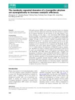
Num. of Labeled Occurrences Correlation
1 - 5 0.022
6 - 10 0.082
11 - 25 0.113
26 - 50 0.183
51 - 75 0.283
76 - 100 0.316
Figure 1: Correlation between Supervised and Un-
supervised Coefficient Estimates
ˆα
j
= log
N
(j,exc.)
/

i:s
i
=1
|d
i
|
N
(j,pr.)
/


i:s
i
=−1
|d
i
|
(20)
= log C
1
+ log N
(j,exc.)
− log N
(j,pr.)
(21)
We generalize this estimate as follows: for a col-
lection of K different anchor words, we consider a
general linear combination of logged co-occurrence
counts.
ˆα
j
=
K

k=1
γ
k
log N
(w
j
,a

k
)
(22)
In the special case of a Naive Bayes model, γ
k
=
1 when the k-th anchor word a
k
conveys positive
sentiment, −1 when it conveys negative sentiment.
Replacing the logit estimate in Equation 9 with
an estimate of this form, the model becomes:

logit(s|d) = ˆα
0
+
p

j=1
d
j
ˆα
j
(23)
= ˆα
0
+
p

j=1

K

k=1
d
j
γ
k
log N
(w
j
,a
k
)
(24)
= γ
0
+
K

k=1
γ
k
p

j=1
d
j
log N
(w
j

,a
k
)
(25)
(26)
This model has only K + 1 parameters:
γ
0
, γ
1
, . . . , γ
K
. These can be learned straightfor-
wardly from labeled documents by a method such
as logistic regression.
Observe that a document receives a score for each
anchor word

p
j=1
d
j
log N
(w
j
,a
k
)
. Effectively, the
predictor variables in this model are no longer

counts of the original features d
j
. Rather, they are
−2.0 −1.5 −1.0 −0.5 0.0 0.5 1.0 1.5
−3 −2 −1 0 1 2 3 4
Traditional Naive Bayes Coefs.
Turney Naive Bayes Coefs.
Unsupervised vs. Supervised Coefficients
Figure 2: Unsupervised versus Supervised Coeffi-
cient Estimates
inner products between the entire feature vector d
and the logged co-occurence vector N
(w,a
k
)
. In this
respect, the vector of logged co-occurrences is used
to produce derived feature.
4 Data Analysis
4.1 Accuracy of Unsupervised Coefficients
By means of a Perl script that uses the Lynx
browser, Version 2.8.3rel.1, we download AltaVista
hit counts for queries of the form “target NEAR
anchor.” The initial list of targets consists of
44,321 word types extracted from the Pang cor-
pus of 1400 labeled movie reviews. After pre-
processing, this number is reduced to 28,629.
3
In Figure 1, we compare estimates produced by
two Naive Bayes procedures. For each feature w

j
,
we estimate α
j
by using Turney’s procedure, and
by fitting a traditional Naive Bayes model to the
labeled documents. The traditional estimates are
smoothed by assuming a Beta prior distribution that
is equivalent to having four previous observations of
w
j
in documents of each class.
ˆq
1j
ˆq
−1j
= C
2
4 +

i:s
i
=1
d
ij
4 +

i:s
i
=−1

d
ij
(27)
where C
2
=
4p +

i:s
i
=1
|d
i
|
4p +

i:s
i
=−1
|d
i
|
(28)
Here, d
ij
is used to indicate feature presence:
d
ij
=


1 if w
j
appears in d
i
0 otherwise
(29)
3
Weeliminate extremely rarewords by requiringeach target
to co-occur at least once with each anchor. In addition, certain
types, such as words containing hyphens, apostrophes, or other
punctuation marks, do not appear to produce valid counts, so
they are discarded.
Positive Negative
best awful
brilliant bad
excellent pathetic
spectacular poor
wonderful worst
Figure 3: Selected Anchor Words
We choose this fitting procedure among several can-
didates because it performs well in classifying test
documents.
In Figure 1, each entry in the right-hand col-
umn is the observed correlation between these two
estimates over a subset of features. For features
that occur in five documents or fewer, the corre-
lation is very weak (0.022). This is not surpris-
ing, as it is difficult to estimate a coefficient from
such a small number of labeled examples. Corre-
lations are stronger for more common features, but

never strong. As a baseline for comparison, Naive
Bayes coefficients can be estimated using a subset
of their labeled occurrences. With two independent
sets of 51-75 occurrences, Naive Bayes coefficient
estimates had a correlation of 0.475.
Figure 2 is a scatterplot of the same coefficient
estimates for word types that appear in 51 to 100
documents. The great majority of features do not
have large coefficients, but even for the ones that
do, there is not a tight correlation.
4.2 Additional Anchors
We wish to learn how our model performance de-
pends on the choice and number of anchor words.
Selecting from WordNet synonym lists (Fellbaum,
1998), we choose five positive anchor words and
five negative (Figure 3). This produces a total of
25 different possible pairs for use in producing co-
efficient estimates.
Figure 4 shows the classification performance
of unsupervised procedures using the 1400 labeled
Pang documents as test data. Coefficients ˆα
j
are es-
timated as described in Equation 22. Several differ-
ent experimental conditions are applied. The meth-
ods labeled ”Count” use the original un-normalized
coefficients, while those labeled “Norm.” have been
normalized so that the number of co-occurrences
with each anchor have identical variance. Results
are shown when rare words (with three or fewer oc-

currences in the labeled corpus) are included and
omitted. The methods “pair” and “10” describe
whether all ten anchor coefficients are used at once,
or just the ones that correspond to a single pair of
Method Feat. Misclass. St.Dev
Count Pair >3 39.6% 2.9%
Norm. Pair >3 38.4% 3.0%
Count Pair all 37.4% 3.1%
Norm. Pair all 37.3% 3.0%
Count 10 > 3 36.4% –
Norm. 10 > 3 35.4% –
Count 10 all 34.6% –
Norm. 10 all 34.1% –
Figure 4: Classification Error Rates for Different
Unsupervised Approaches
anchor words. For anchor pairs, the mean error
across all 25 pairs is reported, along with its stan-
dard deviation.
Patterns are consistent across the different condi-
tions. A relatively large improvement comes from
using all ten anchor words. Smaller benefits arise
from including rare words and from normalizing
model coefficients.
Models that use the original pair of anchor words,
excellent and poor, perform slightly better than the
average pair. Whereas mean performance ranges
from 37.3% to 39.6%, misclassification rates for
this pair of anchors ranges from 37.4% to 38.1%.
4.3 A Smaller Unlabeled Corpus
As described in Section 3.2, there are several rea-

sons to explore the use of a smaller unlabeled cor-
pus, rather than the entire Internet. In our experi-
ments, we use additional movie reviews as our doc-
uments. For this domain, Pang makes available
27,886 reviews.
4
Because this corpus offers dramatically fewer in-
stances of anchor words, we modify our estimation
procedure. Rather than discarding words that rarely
co-occur with anchors, we use the same feature set
as before and regularize estimates by the same pro-
cedure used in the Naive Bayes procedure described
earlier.
Using all features, and ten anchor words with nor-
malized scores, test error is 35.0%. This suggests
that comparable results can be attained while re-
ferring to a considerably smaller unlabeled corpus.
Rather than requiring several days of downloads,
the count of nearby co-occurrences was completed
in under ten minutes.
Because this procedure enables fast access to
counts, we explore the possibility of dramatically
enlarging our collection of anchor words. We col-
4
This corpus is freely available on the following website:
/>100 200 300 400 500 600
0.30 0.32 0.34 0.36 0.38 0.40
Num. of Labeled Documents
Classif. Error
Misclassification versus Sample Size

Figure 5: Misclassification with Labeled Docu-
ments. The solid curve represents a latent fac-
tor model with estimated coefficients. The dashed
curve uses a Naive Bayes classifier. The two hor-
izontal lines represent unsupervised estimates; the
upper one is for the original unsupervised classifier,
and the lower is for the most successful unsuper-
vised method.
lect data for the complete set of WordNet syn-
onyms for the words good, best, bad, boring, and
dreadful. This yields a total of 83 anchor words,
35 positive and 48 negative. When all of these an-
chors are used in conjunction, test error increases to
38.3%. One possible difficulty in using this auto-
mated procedure is that some synonyms for a word
do not carry the same sentiment orientation. For in-
stance, intense is listed as a synonym for bad, even
though its presence in a movie review is a strongly
positive indication.
5
4.4 Methods with Supervision
As demonstrated in Section 3.3, each anchor word
a
k
is associated with a coefficient γ
k
. In unsu-
pervised models, these coefficients are assumed to
be known. However, when labeled documents are
available, it may be advantageous to estimate them.

Figure 5 compares the performance of a model
with estimated coefficient vector γ, as opposed to
unsupervised models and a traditional supervised
approach. When a moderate number of labeled doc-
uments are available, it offers a noticeable improve-
ment.
The supervised method used for reference in this
case is the Naive Bayes model that is described in
section 4.1. Naive Bayes classification is of partic-
ular interest here because it converges faster to its
asymptotic optimum than do discriminative meth-
ods (Ng, A. Y. and Jordan, M., 2002). Further, with
5
In the labeled Pang corpus, intense appears in 38 positive
reviews and only 6 negative ones.
a larger number of labeled documents, its perfor-
mance on this corpus is comparable to that of Sup-
port Vector Machines and Maximum Entropy mod-
els (Pang et al., 2002).
The coefficient vector γ is estimated by regular-
ized logistic regression. This method has been used
in other text classification problems, as in Zhang
and Yang (2003). In our case, the regularization
6
is introduced in order to enforce the beliefs that:
γ
1
≈ γ
2
, if a

1
, a
2
synonyms (30)
γ
1
≈ −γ
2
, if a
1
, a
2
antonyms (31)
For further information on regularized model fitting,
see for instance, Hastie et al. (2001).
5 Conclusion
In business settings, there is growing interest in
learning product reputations from the Internet. For
such problems, it is often difficult or expensive to
obtain labeled data. As a result, a change in mod-
eling strategies is needed, towards approaches that
require less supervision. In this paper we pro-
vide a framework for allowing human-provided in-
formation to be combined with unlabeled docu-
ments and labeled documents. We have found that
this framework enables improvements over existing
techniques, both in terms of the speed of model es-
timation and in classification accuracy. As a result,
we believe that this is a promising new approach to
problems of practical importance.

References
Kushal Dave, Steve Lawrence, and David M. Pen-
nock. 2003. Mining the peanut gallery: Opinion
extraction and semantic classification of product
reviews.
C. Fellbaum. 1998. Wordnet an electronic lexical
database.
T. Hastie, R. Tibshirani, and J. Friedman. 2001.
The Elements of Statistical Learning: Data Min-
ing, Inference, and Prediction. Springer-Verlag.
Vasileios Hatzivassiloglou and Kathleen R. McKe-
own. 1997. Predicting the semantic orientation
of adjectives. In Philip R. Cohen and Wolfgang
Wahlster, editors, Proceedings of the Thirty-Fifth
Annual Meeting of the Association for Computa-
tional Linguistics and Eighth Conference of the
European Chapter of the Association for Com-
putational Linguistics, pages 174–181, Somerset,
New Jersey. Association for Computational Lin-
guistics.
6
By cross-validation, we choose the regularization term λ =
1.5/sqrt(n), where n is the number of labeled documents.
Satoshi Morinaga, Kenji Yamanishi, Kenji Tateishi,
and Toshikazu Fukushima. 2002. Mining prod-
uct reputations on the web.
Ng, A. Y. and Jordan, M. 2002. On discriminative
vs. generative classifiers: A comparison of logis-
tic regression and naive bayes. Advances in Neu-
ral Information Processing Systems, 14.

Kamal Nigam, Andrew K. McCallum, Sebastian
Thrun, and Tom M. Mitchell. 2000. Text clas-
sification from labeled and unlabeled documents
using EM. Machine Learning, 39(2/3):103–134.
Bo Pang, Lillian Lee, and Shivakumar
Vaithyanathan. 2002. Thumbs up? senti-
ment classification using machine learning
techniques. In Proceedings of the 2002 Confer-
ence on Empirical Methods in Natural Language
Processing (EMNLP).
P.D. Turney and M.L. Littman. 2002. Unsupervised
learning of semantic orientation from a hundred-
billion-word corpus.
Peter Turney. 2002. Thumbs up or thumbs down?
semantic orientation applied to unsupervised
classification of reviews. In Proceedings of the
40th Annual Meeting of the Association for
Computational Linguistics (ACL’02), pages 417–
424, Philadelphia, Pennsylvania. Association for
Computational Linguistics.
Janyce Wiebe. 2000. Learning subjective adjec-
tives from corpora. In Proc. 17th National Con-
ference on Artificial Intelligence (AAAI-2000),
Austin, Texas.
Jian Zhang and Yiming Yang. 2003. ”robustness of
regularized linear classification methods in text
categorization”. In Proceedings of the 26th An-
nual International ACM SIGIR Conference (SI-
GIR 2003).