Tài liệu Báo cáo khoa học: "Learning Word Senses With Feature Selection and Order Identification Capabilities" pdf

Learning Word Senses With Feature Selection and Order Identification
Capabilities
Zheng-Yu Niu, Dong-Hong Ji
Institute for Infocomm Research
21 Heng Mui Keng Terrace
119613 Singapore
{zniu, dhji}@i2r.a-star.edu.sg
Chew-Lim Tan
Department of Computer Science
National University of Singapore
3 Science Drive 2
117543 Singapore

Abstract
This paper presents an unsupervised word sense
learning algorithm, which induces senses of target
word by grouping its occurrences into a “natural”
number of clusters based on the similarity of their
contexts. For removing noisy words in feature set,
feature selection is conducted by optimizing a clus-
ter validation criterion subject to some constraint in
an unsupervised manner. Gaussian mixture model
and Minimum Description Length criterion are used
to estimate cluster structure and cluster number.
Experimental results show that our algorithm can
find important feature subset, estimate model or-
der (cluster number) and achieve better performance
than another algorithm which requires cluster num-
ber to be provided.
1 Introduction
Sense disambiguation is essential for many lan-

guage applications such as machine translation, in-
formation retrieval, and speech processing (Ide and
V´eronis, 1998). Almost all of sense disambigua-
tion methods are heavily dependant on manually
compiled lexical resources. However these lexical
resources often miss domain specific word senses,
even many new words are not included inside.
Learning word senses from free text will help us
dispense of outside knowledge source for defining
sense by only discriminating senses of words. An-
other application of word sense learning is to help
enriching or even constructing semantic lexicons
(Widdows, 2003).
The solution of word sense learning is closely re-
lated to the interpretation of word senses. Different
interpretations of word senses result in different so-
lutions to word sense learning.
One interpretation strategy is totreat a word sense
as a set of synonyms like synset in WordNet. The
committee based word sense discovery algorithm
(Pantel and Lin, 2002) followed this strategy, which
treated senses as clusters of words occurring in sim-
ilar contexts. Their algorithm initially discovered
tight clusters called committees by grouping top
n words similar with target word using average-
link clustering. Then the target word was assigned
to committees if the similarity between them was
above a given threshold. Each committee that the
target word belonged to was interpreted as one of
its senses.

There are two difficulties with this committee
based sense learning. The first difficulty is about
derivation of feature vectors. A feature for target
word here consists of a contextual content word and
its grammatical relationship with target word. Ac-
quisition of grammatical relationship depends on
the output of a syntactic parser. But for some lan-
guages, ex. Chinese, the performance of syntactic
parsing is still a problem. The second difficulty with
this solution is that two parameters are required to
be provided, which control the number of commit-
tees and the number of senses of target word.
Another interpretation strategy is to treat a word
sense as a group of similar contexts of target word.
The context group discrimination (CGD) algorithm
presented in (Sch¨utze, 1998) adopted this strategy.
Firstly, their algorithm selected important contex-
tual words using χ
2
or local frequency criterion.
With the χ
2
based criterion, those contextual words
whose occurrence depended on whether the am-
biguous word occurred were chosen as features.
When using local frequency criterion, their algo-
rithm selected top n most frequent contextual words
as features. Then each context of occurrences of
target word was represented by second order co-
occurrence based context vector. Singular value de-

composition (SVD) was conducted to reduce the di-
mensionality of context vectors. Then the reduced
context vectors were grouped into a pre-defined
number of clusters whose centroids corresponded to
senses of target word.
Some observations can be made about their fea-
ture selection and clustering procedure. One ob-
servation is that their feature selection uses only
first order information although the second order co-
occurrence data is available. The other observation
is about their clustering procedure. Similar with
committee based sense discovery algorithm, their
clustering procedure also requires the predefinition
of cluster number. Their method can capture both
coarse-gained and fine-grained sense distinction as
the predefined cluster number varies. But from a
point of statistical view, there should exist a parti-
tioning of data at which the most reliable, “natural”
sense clusters appear.
In this paper, we follow the second order repre-
sentation method for contexts of target word, since
it is supposed to be less sparse and more robust than
first order information (Sch¨utze, 1998). We intro-
duce a cluster validation based unsupervised fea-
ture wrapper to remove noises in contextual words,
which works by measuring the consistency between
cluster structures estimated from disjoint data sub-
sets in selected feature space. It is based on the
assumption that if selected feature subset is impor-
tant and complete, cluster structure estimated from

data subset in this feature space should be stable
and robust against random sampling. After deter-
mination of important contextual words, we use a
Gaussian mixture model (GMM) based clustering
algorithm (Bouman et al., 1998) to estimate cluster
structure and cluster number by minimizing Min-
imum Description Length (MDL) criterion (Ris-
sanen, 1978). We construct several subsets from
widely used benchmark corpus as test data. Experi-
mental results show that our algorithm (FSGMM)
can find important feature subset, estimate cluster
number and achieve better performance compared
with CGD algorithm.
This paper is organized as follows. In section
2 we will introduce our word sense learning al-
gorithm, which incorporates unsupervised feature
selection and model order identification technique.
Then we will give out the experimental results of
our algorithm and discuss some findings from these
results in section 3. Section 4 will be devoted to
a brief review of related efforts on word sense dis-
crimination. In section 5 we will conclude our work
and suggest some possible improvements.
2 Learning Procedure
2.1 Feature selection
Feature selection for word sense learning is to find
important contextual words which help to discrim-
inate senses of target word without using class la-
bels in data set. This problem can be generalized
as selecting important feature subset in an unsuper-

vised manner. Many unsupervised feature selection
algorithms have been presented, which can be cate-
gorized as feature filter (Dash et al., 2002; Talav-
era, 1999) and feature wrapper (Dy and Brodley,
2000; Law et al., 2002; Mitra et al., 2002; Modha
and Spangler, 2003).
In this paper we propose a cluster valida-
tion based unsupervised feature subset evaluation
method. Cluster validation has been used to solve
model order identification problem (Lange et al.,
2002; Levine and Domany, 2001). Table 1 gives
out our feature subset evaluation algorithm. If some
features in feature subset are noises, the estimated
cluster structure on data subset in selected feature
space is not stable, which is more likely to be the
artifact of random splitting. Then the consistency
between cluster structures estimated from disjoint
data subsets will be lower. Otherwise the estimated
cluster structures should be more consistent. Here
we assume that splitting does not eliminate some of
the underlying modes in data set.
For comparison of different clustering structures,
predictors are constructed based on these clustering
solutions, then we use these predictors to classify
the same data subset. The agreement between class
memberships computed by different predictors can
be used as the measure of consistency between clus-
ter structures. We use the stability measure (Lange
et al., 2002) (given in Table 1) to assess the agree-
ment between class memberships.

For each occurrence, one strategy is to construct
its second order context vector by summing the vec-
tors of contextual words, then let the feature selec-
tion procedure start to work on these second order
contextual vectors toselect features. However, since
the sense associated with a word’s occurrence is al-
ways determined by very few feature words in its
contexts, it is always the case that there exist more
noisy words than the real features in the contexts.
So, simply summing the contextual word’s vectors
together may result in noise-dominated second or-
der context vectors.
To deal with this problem, we extend the feature
selection procedure further to the construction of
second order context vectors: to select better feature
words in contexts to construct better second order
context vectors enabling better feature selection.
Since the sense associated with a word’s occur-
rence is always determined by some feature words
in its contexts, it is reasonable to suppose that the
selected features should cover most of occurrences.
Formally, let coverag e(D, T) be the coverage rate
of the feature set T with respect to a set of con-
texts D, i.e., the ratio of the number of the occur-
rences with at least one feature in their local con-
texts against the total number of occurrences, then
we assume that coverage(D, T ) ≥ τ . In practice,
we set τ = 0.9.
This assumption also helps to avoid the bias to-
ward the selection of fewer features, since with

fewer features, there are more occurrences without
features in contexts, and their context vectors will
be zero valued, which tends to result in more stable
cluster structure.
Let D be a set of local contexts of occurrences of
target word, then D = {d
i
}
N
i=1
, where d
i
represents
local context of the i-th occurrence, and N is the
total number of this word’s occurrences.
W is used to denote bag of words occurring in
context set D, then W = {w
i
}
M
i=1
, where w
i
de-
notes a word occurring in D, and M is the total
number of different contextual words.
Let V denote a M × M second-order co-
occurrence symmetric matrix. Suppose that the i-th
, 1 ≤ i ≤ M, row in the second order matrix corre-
sponds to word w

i
and the j-th , 1 ≤ j ≤ M , col-
umn corresponds to word w
j
, then the entry speci-
fied by i-th row and j-th column records the number
of times that word w
i
occurs close to w
j
in corpus.
We use v(w
i
) to represent the word vector of con-
textual word w
i
, which is the i-th row in matrix V .
H
T
is a weight matrix of contextual word subset
T , T ⊆ W . Then each entry h
i,j
represents the
weight of word w
j
in d
i
, w
j
∈ T , 1 ≤ i ≤ N. We

use binary term weighting method to derive context
vectors: h
i,j
= 1 if word w
j
occurs in d
i
, otherwise
zero.
Let C
T
= {c
T
i
}
N
i=1
be a set of context vectors in
feature space T , where c
T
i
is the context vector of
the i-th occurrence. c
T
i
is defined as:
c
T
i
=


j
(h
i,j
v(w
j
)), w
j
∈ T, 1 ≤ i ≤ N. (1)
The feature subset selection in word set W can be
formulated as:
ˆ
T = arg max
T
{cr iterion(T, H, V, q)}, T ⊆ W, (2)
subject to coverage(D, T) ≥ τ , where
ˆ
T is the op-
timal feature subset, criterion is the cluster valida-
tion based evaluation function (the function in Ta-
ble 1), q is the resampling frequency for estimate
of stability, and coverage(D, T ) is the proportion
of contexts with occurrences of features in T . This
constrained optimization results in a solution which
maximizes the criterion and meets the given con-
straint at the same time. In this paper we use se-
quential greedy forward floating search (Pudil et al.,
1994) in sorted word list based on χ
2
or local fre-

quency criterion. We set l = 1, m = 1, where l is
plus step, and m is take-away step.
2.2 Clustering with order identification
After feature selection, we employ a Gaussian mix-
ture modelling algorithm, Cluster (Bouman et al.,
Table 1: Unsupervised Feature Subset Evaluation Algorithm.
Intuitively, for a given feature subset T , we iteratively split data
set into disjoint halves, and compute the agreement of cluster-
ing solutions estimated from these sets using stability measure.
The average of stability over q resampling is the estimation of
the score of T .
Function criterion(T , H, V , q)
Input parameter: feature subset T , weight matrix H,
second order co-occurrence matrix V , resampling
frequency q;
(1) S
T
= 0;
(2) For i = 1 to q do
(2.1) Randomly split C
T
into disjoint halves, denoted
as C
T
A
and C
T
B
;
(2.2) Estimate GMM parameter and cluster number on C

T
A
using Cluster, and the parameter set is denoted as
ˆ
θ
A
;
The solution
ˆ
θ
A
can be used to construct a predictor
ρ
A
;
(2.3) Estimate GMM parameter and cluster number on C
T
B
using Cluster, and the parameter set is denoted as
ˆ
θ
B
,
The solution
ˆ
θ
B
can be used to construct a predictor
ρ
B

;
(2.4) Classify C
T
B
using ρ
A
and ρ
B
;
The class labels assigned by ρ
A
and ρ
B
are denoted
as L
A
and L
B
;
(2.5) S
T
+ = max
π
1
|C
T
B
|

i

1{π(L
A
(c
T
Bi
)) = L
B
(c
T
Bi
)},
where π denotes possible permutation relating indices
between L
A
and L
B
, and c
T
Bi
∈ C
T
B
;
(3) S
T
=
1
q
S
T

;
(4) Return S
T
;
1998), to estimate cluster structure and cluster num-
ber. Let Y = {y
n
}
N
n=1
be a set of M dimen-
sional vectors to be modelled by GMM. Assuming
that this model has K subclasses, let π
k
denote the
prior probability of subclass k, µ
k
denote the M di-
mensional mean vector for subclass k, R
k
denote
the M × M dimensional covariance matrix for sub-
class k, 1 ≤ k ≤ K. The subclass label for pixel
y
n
is represented by x
n
. MDL criterion is used
for GMM parameter estimation and order identifi-
cation, which is given by:

MDL(K, θ) = −
N

n=1
log (p
y
n
|x
n
(y
n
|Θ)) +
1
2
L log (NM ),
(3)
p
y
n
|x
n
(y
n
|Θ) =
K

k=1
p
y
n

|x
n
(y
n
|k, θ)π
k
, (4)
L = K(1 + M +
(M + 1)M
2
) − 1, (5)
The log likelihood measures the goodness of fit of
a model to data sample, while the second term pe-
nalizes complex model. This estimator works by at-
tempting to find a model order with minimum code
length to describe the data sample Y and parameter
set Θ.
If the cluster number is fixed, the estimation of
GMM parameter can be solved using EM algorithm
to address this type of incomplete data problem
(Dempster et al., 1977). The initialization of mix-
ture parameter θ
(1)
is given by:
π
(1)
k
=
1
K

o
(6)
µ
(1)
k
= y
n
, where n = (k − 1)(N − 1)/(K
o
− 1) + 1 (7)
R
(1)
k
=
1
N
Σ
N
n=1
y
n
y
t
n
(8)
K
o
is a given initial subclass number.
Then EM algorithm is used to estimate model pa-
rameters by minimizing MDL:

E-step: re-estimate the expectations based on pre-
vious iteration:
p
x
n
|y
n
(k|y
n
, θ
(i)
) =
p
y
n
|x
n
(y
n
|k, θ
(i)
)π
k

K
l=1
(p
y
n
|x

n
(y
n
|l, θ
(i)
)π
l
)
, (9)
M-step: estimate the model parameter θ
(i)
to
maximize the log-likelihood in MDL:
N
k
=
N

n=1
p
x
n
|y
n
(k|y
n
, θ
(i)
) (10)
π

k
=
N
k
N
(11)
µ
k
=
1
N
k
N

n=1
y
n
p
x
n
|y
n
(k|y
n
, θ
(i)
) (12)
R
k
=

1
N
k
N

n=1
(y
n
− µ
k
)(y
n
− µ
k
)
t
p
x
n
|y
n
(k|y
n
, θ
(i)
)
(13)
p
y
n

|x
n
(y
n
|k, θ
(i)
) =
1
(2π)
M/2
|R
k
|
−1/2
exp{λ} (14)
λ = −
1
2
(y
n
−
µ
k
)
t
R
−1
k
(y
n

− µ
k
) (15)
The EM iteration is terminated when the change
of MDL(K, θ) is less than :
 =
1
100
(1 + M +
(M + 1)M
2
)log(NM ) (16)
For inferring the cluster number, EM algorithm
is applied for each value of K, 1 ≤ K ≤ K
o
, and
the value
ˆ
K which minimizes the value of MDL
is chosen as the correct cluster number. To make
this process more efficient, two cluster pair l and m
are selected to minimize the change in MDL crite-
ria when reducing K to K − 1. These two clusters
l and m are then merged. The resulting parameter
set is chosen as an initial condition for EM iteration
with K − 1 subclasses. This operation will avoid a
complete minimization with respect to π, µ, and R
for each value of K.
Table 2: Four ambiguous words, their senses and frequency
distribution of each sense.

Word Sense Percentage
hard not easy (difficult) 82.8%
(adjective) not soft (metaphoric) 9.6%
not soft (physical) 7.6%
interest money paid for the use of money 52.4%
a share in a company or business 20.4%
readiness to give attention 14%
advantage, advancement or favor 9.4%
activity that one gives attention to 3.6%
causing attention to be given to 0.2%
line product 56%
(noun) telephone connection 10.6%
written or spoken text 9.8%
cord 8.6%
division 8.2%
formation 6.8%
serve supply with food 42.6%
(verb) hold an office 33.6%
function as something 16%
provide a service 7.8%
3 Experiments and Evaluation
3.1 Test data
We constructed four datasets from hand-tagged cor-
pus
1
by randomly selecting 500 instances for each
ambiguous word - “hard”, “interest”, “line”, and
“serve”. The details of these datasets are given in
Table 2. Our preprocessing included lowering the
upper case characters, ignoring all words that con-

tain digits or non alpha-numeric characters, remov-
ing words from a stop word list, and filtering out
low frequency words which appeared only once in
entire set. We did not use stemming procedure.
The sense tags were removed when they were used
by F SGM M and CGD. In evaluation procedure,
these sense tags were used as ground truth classes.
A second order co-occurrence matrix for English
words was constructed using English version of
Xinhua News (Jan. 1998-Dec. 1999). The win-
dow size for counting second order co-occurrence
was 50 words.
3.2 Evaluation method for feature selection
For evaluation of feature selection, we used mutual
information between feature subset and class label
set to assess the importance of selected feature sub-
set. Our assessment measure is defined as:
M(T ) =
1
|T |

w∈T

l∈L
p(w, l)log
p(w, l)
p(w)p(l)
, (17)
where T is the feature subset to be evaluated, T ⊆
W , L is class label set, p(w, l) is the joint distri-

bution of two variables w and l, p(w) and p(l) are
marginal probabilities. p(w , l) is estimated based
1
/>on contingency table of contextual word set W and
class label set L. Intuitively, if M(T
1
) > M (T
2
),
T
1
is more important than T
2
since T
1
contains more
information about L.
3.3 Evaluation method for clustering result
When assessing the agreement between clustering
result and hand-tagged senses (ground truth classes)
in benchmark data, we encountered the difficulty
that there was no sense tag for each cluster.
In (Lange et al., 2002), they defined a permu-
tation procedure for calculating the agreement be-
tween two cluster memberships assigned by differ-
ent unsupervised learners. In this paper, we applied
their method to assign different sense tags to only
min(|U|, |C|) clusters by maximizing the accuracy,
where |U | is the number of clusters, and |C| is the
number of ground truth classes. The underlying as-

sumption here is that each cluster is considered as
a class, and for any two clusters, they do not share
same class labels. At most |C| clusters are assigned
sense tags, since there are only |C| classes in bench-
mark data.
Given the contingency table Q between clusters
and ground truth classes, each entry Q
i,j
gives the
number of occurrences which fall into both the i-
th cluster and the j-th ground truth class. If |U| <
|C|, we constructed empty clusters so that |U| =
|C|. Let Ω represent a one-to-one mapping function
from C to U. It means that Ω(j
1
) = Ω(j
2
) if j
1
=
j
2
and vice versa, 1 ≤ j
1
, j
2
≤ |C|. Then Ω(j)
is the index of the cluster associated with the j-th
class. Searching a mapping function to maximize
the accuracy of U can be formulated as:

ˆ
Ω = arg max
Ω
|C|

j=1
Q
Ω(j),j
. (18)
Then the accuracy of solution U is given by
Accur acy(U ) =

j
Q
ˆ
Ω(j),j

i,j
Q
i,j
. (19)
In fact,

i,j
Q
i,j
is equal to N, the number of
occurrences of target word in test set.
3.4 Experiments and results
For each dataset, we tested following procedures:

CGD
term
:We implemented the context group
discrimination algorithm. Top max(|W | ×
20%, 100) words in contextual word list was se-
lected as features using frequency or χ
2
based rank-
ing. Then k-means clustering
2
was performed on
context vector matrix using normalized Euclidean
distance. K-means clustering was repeated 5 times
2
We used k-means function in statistics toolbox of Matlab.
and the partition with best quality was chosen as fi-
nal result. The number of clusters used by k-means
was set to be identical with the number of ground
truth classes. We tested CGD
term
using various
word vector weighting methods when deriving con-
text vectors, ex. binary, idf, tf · idf .
CGD
SV D
: The context vector matrix was de-
rived using same method in CGD
term
. Then k-
means clustering was conducted on latent seman-

tic space transformed from context vector matrix,
using normalized Euclidean distance. Specifically,
context vectors were reduced to 100 dimensions us-
ing SVD. If the dimension of context vector was
less than 100, all of latent semantic vectors with
non-zero eigenvalue were used for subsequent clus-
tering. We also tested it using different weighting
methods, ex. binary, idf, tf · idf.
F SGMM : We performed cluster validation
based feature selection in feature set used by CGD.
Then Cluster algorithm was used to group target
word’s instances using Euclidean distance measure.
τ was set as 0.90 in feature subset search procedure.
The random splitting frequency is set as 10 for es-
timation of the score of feature subset. The initial
subclass number was 20 and full covariance matrix
was used for parameter estimation of each subclass.
For investigating the effect of different context
window size on the performance of three proce-
dures, we tested these procedures using various con-
text window sizes: ±1, ±5, ±15, ±25, and all of
contextual words. The average length of sentences
in 4 datasets is 32 words before preprocessing. Per-
formance on each dataset was assessed by equation
19.
The scores of feature subsets selected by
F SGMM and CGD are listed in Table 3 and
4. The average accuracy of three procedures with
different feature ranking and weighting method is
given in Table 5. Each figure is the average over 5

different context window size and 4 datasets. We
give out the detailed results of these three proce-
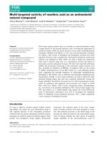
dures in Figure 1. Several results should be noted
specifically:
From Table 3 and 4, we can find that F SGMM
achieved better score on mutual information (MI)
measure than CGD over 35 out of total 40 cases.
This is the evidence that our feature selection pro-
cedure can remove noise and retain important fea-
tures.
As it was shown in Table 5, with both χ
2
and
freq based feature ranking, F SGM M algorithm
performed better than CGD
term
and CGD
SV D
if
we used average accuracy to evaluate their per-
formance. Specifically, with χ
2
based feature
ranking, F SGMM attained 55.4% average accu-
racy, while the best average accuracy of CGD
term
and CGD
SV D
were 40.9% and 51.3% respec-
tively. With freq based feature ranking, FSGMM

achieved 51.2% average accuracy, while the best av-
erage accuracy of CGD
term
and CGD
SV D
were
45.1% and 50.2%.
The automatically estimated cluster numbers by
F SGMM over 4 datasets are given in Table 6.
The estimated cluster number was 2 ∼ 4 for “hard”,
3 ∼ 6 for “interest”, 3 ∼ 6 for “line”, and 2 ∼ 4
for “serve”. It is noted that the estimated cluster
number was less than the number of ground truth
classes in most cases. There are some reasons for
this phenomenon. First, the data is not balanced,
which may lead to that some important features can-
not be retrieved. For example, the fourth sense of
“serve”, and the sixth sense of “line”, their corre-
sponding features are not up to the selection criteria.
Second, some senses can not be distinguished using
only bag-of-words information, and their difference
lies in syntactic information held by features. For
example, the third sense and the sixth sense of “in-
terest” may be distinguished by syntactic relation of
feature words, while the bag of feature words occur-
ring in their context are similar. Third, some senses
are determined by global topics, rather than local
contexts. For example, according to global topics, it
may be easier to distinguish the first and the second
sense of “interest”.

Figure 2 shows the average accuracy over three
procedures in Figure 1 as a function of context
window size for 4 datasets. For “hard”, the per-
formance dropped as window size increased, and
the best accuracy(77.0%) was achieved at win-
dow size 1. For “interest”, sense discrimination
did not benefit from large window size and the
best accuracy(40.1%) was achieved at window size
5. For “line”, accuracy dropped when increas-
ing window size and the best accuracy(50.2%) was
achieved at window size 1. For “serve”, the per-
formance benefitted from large window size and the
best accuracy(46.8%) was achieved at window size
15.
In (Leacock et al., 1998), they used Bayesian ap-
proach for sense disambiguation of three ambiguous
words, “hard”, “line”, and “serve”, based on cues
from topical and local context. They observed that
local context was more reliable than topical context
as an indicator of senses for this verb and adjective,
but slightly less reliable for this noun. Compared
with their conclusion, we can find that our result
is consistent with it for “hard”. But there is some
differences for verb “serve” and noun “line”. For
Table 3: Mutual information between feature subset and class
label with χ
2
based feature ranking.
Word Cont. Size of MI Size of MI
wind. feature ×10

−2
feature ×10
−2
size subset subset
of CGD of
FSGMM
hard 1 18 6.4495 14 8.1070
5 100 0.4018 80 0.4300
15 100 0.1362 80 0.1416
25 133 0.0997 102 0.1003
all 145 0.0937 107 0.0890
interest 1 64 1.9697 55 2.0639
5 100 0.3234 89 0.3355
15 157 0.1558 124 0.1531
25 190 0.1230 138 0.1267
all 200 0.1163 140 0.1191
line 1 39 4.2089 32 4.6456
5 100 0.4628 84 0.4871
15 183 0.1488 128 0.1429
25 263 0.1016 163 0.0962
all 351 0.0730 192 0.0743
serve 1 22 6.8169 20 6.7043
5 100 0.5057 85 0.5227
15 188 0.2078 164 0.2094
25 255 0.1503 225 0.1536
all 320 0.1149 244 0.1260
Table 4: Mutual information between feature subset and class
label with freq based feature ranking.
Word Cont. Size of MI Size of MI
wind. feature ×10

−2
feature ×10
−2
size subset subset
of CGD of
FSGMM
hard 1 18 6.4495 14 8.1070
5 100 0.4194 80 0.4832
15 100 0.1647 80 0.1774
25 133 0.1150 102 0.1259
all 145 0.1064 107 0.1269
interest 1 64 1.9697 55 2.7051
5 100 0.6015 89 0.8309
15 157 0.2526 124 0.3495
25 190 0.1928 138 0.2982
all 200 0.1811 140 0.2699
line 1 39 4.2089 32 4.4606
5 100 0.6895 84 0.7816
15 183 0.2301 128 0.2929
25 263 0.1498 163 0.2181
all 351 0.1059 192 0.1630
serve 1 22 6.8169 20 7.0021
5 100 0.7045 85 0.8422
15 188 0.2763 164 0.3418
25 255 0.1901 225 0.2734
all 320 0.1490 244 0.2309
“serve”, the possible reason is that we do not use
position of local word and part of speech informa-
tion, which may deteriorate the performance when
local context(≤ 5 words) is used. For “line”, the

reason might come from the feature subset, which
is not good enough to provide improvement when
Table 5: Average accuracy of three procedures with various
settings over 4 datasets.
Algorithm Feature Feature Average
ranking weighting accuracy
method method
F SGMM χ
2
binar y 0.554
CGD
term
χ
2
binar y 0.404
CGD
term
χ
2
idf 0.407
CGD
term
χ
2
tf · idf 0.409
CGD
SV D
χ
2
binar y 0.513

CGD
SV D
χ
2
idf 0.512
CGD
SV D
χ
2
tf · idf 0.508
F SGMM freq binary 0.512
CGD
term
freq binary 0.451
CGD
term
freq idf 0.437
CGD
term
freq tf · idf 0.447
CGD
SV D
freq binary 0.502
CGD
SV D
freq idf 0.498
CGD
SV D
freq tf · idf 0.485
Table 6: Automatically determined mixture component num-

ber.
Word Context Model Model
window order order
size with χ
2
with freq
hard 1 3 4
5 2 2
15 2 3
25 2 3
all 2 3
interest 1 5 4
5 3 4
15 4 6
25 4 6
all 3 4
line 1 5 6
5 4 3
15 5 4
25 5 4
all 3 4
serve 1 3 3
5 3 4
15 3 3
25 3 3
all 2 4
context window size is no less than 5.
4 Related Work
Besides the two works (Pantel and Lin, 2002;
Sch¨utze, 1998), there are other related efforts on

word sense discrimination (Dorow and Widdows,
2003; Fukumoto and Suzuki, 1999; Pedersen and
Bruce, 1997).
In (Pedersen and Bruce, 1997), they described an
experimental comparison of three clustering algo-
rithms for word sense discrimination. Their feature
sets included morphology of target word, part of
speech of contextual words, absence or presence of
particular contextual words, and collocation of fre-
0 1 5 15 25 all
0.4
0.5
0.6
0.7
0.8
0.9
Hard dataset
Accuracy
0 1 5 15 25 all
0.2
0.3
0.4
0.5
0.6
Accuracy
Interest dataset
0 1 5 15 25 all
0.2
0.3
0.4

0.5
0.6
0.7
Line dataset
Accuracy
0 1 5 15 25 all
0.3
0.35
0.4
0.45
0.5
0.55
0.6
Serve dataset
Accuracy
Figure 1: Results for three procedures over 4 datases. The
horizontal axis corresponds to the context window size. Solid
line represents the result of F SGM M + binary, dashed line
denotes the result of CGD
SV D
+ idf, and dotted line is the
result of CGD
term
+ idf. Square marker denotes χ
2
based
feature ranking, while cross marker denotes freq based feature
ranking.
0 1 5 15 25 all
0.3

0.35
0.4
0.45
0.5
0.55
0.6
0.65
0.7
0.75
0.8
Average Accuracy
Hard dataset
Interest dataset
Line dataset
Serve dataset
Figure 2: Average accuracy over three procedures in Figure
1 as a function of context window size (horizontal axis) for 4
datasets.
quent words. Then occurrences of target word were
grouped into a pre-defined number of clusters. Sim-
ilar with many other algorithms, their algorithm also
required the cluster number to be provided.
In (Fukumoto and Suzuki, 1999), a term weight
learning algorithm was proposed for verb sense dis-
ambiguation, which can automatically extract nouns
co-occurring with verbs and identify the number of
senses of an ambiguous verb. The weakness of their
method is to assume that nouns co-occurring with
verbs are disambiguated in advance and the number
of senses of target verb is no less than two.

The algorithm in (Dorow and Widdows, 2003)
represented target noun word, its neighbors and
their relationships using a graph in which each node
denoted a noun and two nodes had an edge between
them if they co-occurred with more than a given
number of times. Then senses of target word were
iteratively learned by clustering the local graph of
similar words around target word. Their algorithm
required a threshold as input, which controlled the
number of senses.
5 Conclusion and Future Work
Our word sense learning algorithm combined two
novel ingredients: feature selection and order iden-
tification. Feature selection was formalized as a
constrained optimization problem, the output of
which was a set of important features to determine
word senses. Both cluster structure and cluster num-
ber were estimated by minimizing a MDL crite-
rion. Experimental results showed that our algo-
rithm can retrieve important features, estimate clus-
ter number automatically, and achieve better per-
formance in terms of average accuracy than CGD
algorithm which required cluster number as input.
Our word sense learning algorithm is unsupervised
in two folds: no requirement of sense tagged data,
and no requirement of predefinition of sense num-
ber, which enables the automatic discovery of word
senses from free text.
In our algorithm, we treat bag of words in lo-
cal contexts as features. It has been shown that

local collocations and morphology of target word
play important roles in word sense disambiguation
or discrimination (Leacock et al., 1998; Widdows,
2003). It is necessary to incorporate these more
structural information to improve the performance
of word sense learning.
References
Bouman, C. A., Shapiro, M., Cook, G. W., Atkins,
C. B., & Cheng, H. (1998) Cluster: An
Unsupervsied Algorithm for Modeling Gaus-
sian Mixtures. />∼bouman/software/cluster/.
Dash, M., Choi, K., Scheuermann, P., & Liu, H. (2002)
Feature Selection for Clustering - A Filter Solution.
Proc. of IEEE Int. Conf. on Data Mining(pp. 115–
122).
Dempster, A. P., Laird, N. M., & Rubin, D. B. (1977)
Maximum likelihood from incomplete data using the
EM algorithm. Journal of the Royal Statistical Soci-
ety, 39(B).
Dorow, B, & Widdows, D. (2003) Discovering Corpus-
Specific Word Senses. Proc. of the 10th Conf. of the
European Chapter of the Association for Computa-
tional Linguistics, Conference Companion (research
notes and demos)(pp.79–82).
Dy, J. G., & Brodley, C. E. (2000) Feature Subset Selec-
tion and Order Identification for Unsupervised Learn-
ing. Proc. of the 17th Int. Conf. on Machine Learn-
ing(pp. 247–254).
Fukumoto, F., & Suzuki, Y. (1999) Word Sense Disam-
biguation in Untagged Text Based on Term Weight

Learning. Proc. of the 9th Conf. of European Chapter
of the Association for Computational Linguistics(pp.
209–216).
Ide, N., & V´eronis, J. (1998) Word Sense Disambigua-
tion: The State of the Art. Computational Linguistics,
24:1, 1–41.
Lange, T., Braun, M., Roth, V., & Buhmann, J. M. (2002)
Stability-Based Model Selection. Advances in Neural
Information Processing Systems 15.
Law, M. H., Figueiredo, M., & Jain, A. K. (2002) Fea-
ture Selection in Mixture-Based Clustering. Advances
in Neural Information Processing Systems 15.
Leacock, C., Chodorow, M., & Miller A. G. (1998) Us-
ing CorpusStatistics andWordNet Relationsfor Sense
Identification. Computational Linguistics, 24:1, 147–
165.
Levine, E., & Domany, E. (2001) Resampling Method
for Unsupervised Estimation of Cluster Validity. Neu-
ral Computation, Vol. 13, 2573–2593.
Mitra, P., Murthy, A. C., & Pal, K. S. (2002) Unsu-
pervised Feature Selection Using Feature Similarity.
IEEE Transactions on Pattern Analysis and Machine
Intelligence, 24:4, 301–312.
Modha, D. S., & Spangler, W. S. (2003) Feature Weight-
ing in k-Means Clustering. Machine Learning, 52:3,
217–237.
Pantel, P. & Lin, D. K. (2002) Discovering Word Senses
from Text. Proc. of ACM SIGKDD Conf. on Knowl-
edge Discovery and Data Mining(pp. 613-619).
Pedersen, T., & Bruce, R. (1997) Distinguishing Word

Senses in Untagged Text. Proceedings of the 2nd
Conference on Empirical Methods in Natural Lan-
guage Processing(pp. 197–207).
Pudil, P., Novovicova, J., & Kittler, J. (1994) Floating
Search Methods in Feature Selection. Pattern Recog-
nigion Letters, Vol. 15, 1119-1125.
Rissanen, J. (1978) Modeling by Shortest Data Descrip-
tion. Automatica, Vol. 14, 465–471.
Sch¨utze, H. (1998) Automatic Word Sense Discrimina-
tion. Computational Linguistics, 24:1, 97–123.
Talavera, L. (1999) Feature Selection as a Preprocessing
Step for Hierarchical Clustering. Proc. of the 16th Int.
Conf. on Machine Learning(pp. 389–397).
Widdows, D. (2003) Unsupervised methods for devel-
oping taxonomies by combining syntactic and statisti-
cal information. Proc. of the Human Language Tech-
nology / Conference of the North American Chapter
of the Association for Computational Linguistics(pp.
276–283).