Tài liệu Báo cáo khoa học: "Methods for the Qualitative Evaluation of Lexical Association Measures" doc

Methods for the Qualitative Evaluation of Lexical Association Measures
Stefan Evert
IMS, University of Stuttgart
Azenbergstr. 12
D-70174 Stuttgart, Germany

Brigitte Krenn
Austrian Research Institute
for Artificial Intelligence (ÖFAI)
Schottengasse 3
A-1010 Vienna, Austria

Abstract
This paper presents methods for a qual-
itative, unbiased comparison of lexical
association measures and the results we
have obtained for adjective-noun pairs
and preposition-noun-verb triples ex-
tracted from German corpora. In our
approach, we compare the entire list
of candidates, sorted according to the
particular measures, to a reference set
of manually identified “true positives”.
We also show how estimates for the
very large number of hapaxlegomena
and double occurrences can be inferred
from random samples.
1 Introduction
In computational linguistics, a variety of (statis-
tical) measures have been proposed for identify-
ing lexical associations between words in lexi-

cal tuples extracted from text corpora. Methods
used range from pure frequency counts to infor-
mation theoretic measures and statistical signifi-
cance tests. While the mathematical properties of
those measures have been extensively discussed,
1
the strategies employed for evaluating the iden-
tification results are far from adequate. Another
crucial but still unsolved issue in statistical col-
location identification is the treatment of low-
frequency data.
In this paper, we firstspecify requirements for a
qualitative evaluation of lexical association mea-
1
See for instance (Manning and Schütze, 1999, chap-
ter 5), (Kilgarriff, 1996), and (Pedersen, 1996).
sures (AMs). Based on these requirements, we
introduce an experimentation procedure, and dis-
cuss the evaluation results for a number of widely
used AMs. Finally, methods and strategies for
handling low-frequency data are suggested.
The measures
2
– Mutual Information (
)
(Church and Hanks, 1989), the log-likelihood
ratio test (Dunning, 1993), two statistical tests:
t-test and
-test, and co-occurrence frequency –
are applied to two sets of data: adjective-noun

(AdjN) pairs and preposition-noun-verb (PNV)
triples, where the AMs are applied to (PN,V)
pairs. See section 3 for a description of the base
data. For evaluation of the association measures,
-best strategies (section 4.1) are supplemented
with precision and recall graphs (section 4.2) over
the complete data sets. Samples comprising par-
ticular frequency strata (high versus low frequen-
cies) are examined (section 4.3). In section 5,
methods for the treatment of low-frequency data,
single (hapaxlegomena) and double occurrences
are discussed. The significance of differences be-
tween the AMs is addressed in section 6.
2 The Qualitative Evaluation of
Association Measures
2.1 State-of-the-art
A standard procedure for the evaluation of AMs is
manual judgment of the -best candidates identi-
fied in a particular corpus by the measure in ques-
tion. Typically, the number of true positives (TPs)
2
For a more detailed description of these measures
and relevant literature, see (Manning and Schütze, 1999,
chapter 5) or />where several other AMs are discussed as well.
among the 50 or 100 (or slightly more) highest
ranked word combinations is manually identified
by a human evaluator, in most cases the author
of the paper in which the evaluation is presented.
This method leads to a very superficial judgment
of AMs for the following reasons:

(1) The identification results are based on small
subsets of the candidates extracted from the cor-
pus. Consequently, results achieved by individ-
ual measures may very well be due to chance (cf.
sections 4.1 and 4.2), and evaluation with respect
to frequency strata is not possible (cf. section
4.3). (2) For the same reason, it is impossible
to determine recall values, which are important
for many practical applications. (3) The introduc-
tion of new measures or changes to the calculation
methods require additional manual evaluation, as
new
-best lists are generated.
2.2 Requirements
To improve the reliability of the evaluation re-
sults, a number of properties need to be con-
trolled. We distinguish between two classes:
(1) Characteristics of the set of candidate data
employed for collocation identification: (i) the
syntactic homogeneity of the base data, i.e.,
whether the set of candidate data consists only of
adjective-noun, noun-verb, etc. pairs or whether
different types of word combinations are mixed;
(ii) the grammatical status of the individual word
combinations in the base set, i.e., whether they
are part of or constitute a phrase or simply co-
occur within a given text window; (iii) the per-
centage of TPs in the base set, which is typically
higher among high-frequency data than among
low-frequency data.

(2) The evaluation strategies applied: Instead
of examining only a small sample of
-best can-
didates for each measure as it is common practice,
we make use of recall and precision values for -
best samples of arbitrary size, which allows us to
plot recall and precision curves for the whole set
of candidate data. In addition, we compare preci-
sion curves for different frequency strata.
3 The Base Data
The base data for our experiments are extracted
from two corpora which differ with respect to size
and text type. The base sets also differ with re-
spect to syntactic homogeneity and grammatical
correctness. Both candidate sets have been man-
ually inspected for TPs.
The first set comprises bigrams of adjacent,
lemmatized AdjN pairs extracted from a small
(
word) corpus of freely available Ger-
man law texts.
3
Due to the extraction strategy, the
data are homogeneous and grammatically correct,
i.e., there is (almost) always a grammatical de-
pendency between adjacent adjectives and nouns
in running text. Two human annotators indepen-
dently marked candidate pairs perceived as “typ-
ical” combinations, including idioms ((die) hohe
See, ‘the high seas’), legal terms (üble Nachrede,

‘slander’), and proper names (Rotes Kreuz, ‘Red
Cross’). Candidates accepted by either one of the
annotators were considered TPs.
The second set consists of PNV triples ex-
tracted from an 8 million word portion of the
Frankfurter Rundschau Corpus
4
, in which part-
of-speech tags and minimal PPs were identified.
5
The PNV triples were selected automatically such
that the preposition and the noun are constituents
of the same PP, and the PP and the verb co-occur
within a sentence. Only main verbs were con-
sidered and full forms were reduced to bases.
6
The PNV data are partially inhomogeneous and
not fully grammatically correct, because they in-
clude combinations with no grammatical relation
between PN and V. PNV collocations were man-
ually annotated. The criteria used for the dis-
tinction between collocations and arbitrary word
combinations are: There is a grammatical rela-
tion between the verb and the PP, and the triple
can be interpreted as support verb construction
and/or a metaphoric or idiomatic reading is avail-
able, e.g.: zur Verfügung stellen (at_the availabil-
ity put, ‘make available’), am Herzen liegen (at
the heart lie, ‘have at heart’).
7

3
See (Schmid, 1995) for a description of the part-of-
speech tagger used to identify adjectives and nouns in the
corpus.
4
The Frankfurter Rundschau Corpus is part of the Euro-
pean Corpus Initiative Multilingual Corpus I.
5
See (Skut and Brants, 1998) for a description of the tag-
ger and chunker.
6
Mmorph – theMULTEXT morphology tool provided by
ISSCO/SUISSETRA, Geneva, Switzerland – has been em-
ployed for determining verb infinitives.
7
For definitions of and literature on idioms, metaphors
and support verb constructions (Funktionsverbgefüge) see
for instance (Bußmann, 1990).
AdjN data PNV data
total 11 087 total 294 534
4 652 14 654
colloc. 15.84% colloc. 6.41%
= 737 = 939
Table 1: Base sets used for evaluation
General statistics for the AdjN and PNV base
sets are given in Table 1. Manual annotation was
performed for AdjN pairs with frequency
and PNV triples with only (see section
5 for a discussion of the excluded low-frequency
candidates).

4 Experimental Setup
After extraction of the base data and manual iden-
tification of TPs, the AMs are applied, resulting in
an ordered candidate list for each measure (hence-
forth significance list, SL). The order indicates the
degree of collocativity. Multiple candidates with
identical scores are listed in random order. This is
necessary, in particular, when co-occurrence fre-
quency is used as an association measure.
4.1
-Best Lists
In this approach, the set of the highest ranked
word combinations is evaluated for each measure,
and the proportion of TPs among this -best list
(the precision) is computed. Another measure of
goodness is the proportion of TPs in the base data
that are also contained in the -best list (the re-
call). While precision measures the quality of the
-best lists produced, recall measures their cov-
erage, i.e., how many of all true collocations in
the corpus were identified. The most problematic
aspect here is that conclusions drawn from -best
lists for a single (and often small) value of are
only snapshots and likely to be misleading.
For instance, considering the set of AdjN base
data with we might arrive at the following
results (Table 2 gives the precision values of the
highest ranked word combinations with
): As expected from the results of other
studies (e.g. Lezius (1999)), the precision of

is significantly lower than that of log-likelihood,
8
8
This is to a large part due to the fact that systemati-
cally overestimates the collocativity of low-frequency pairs,
cf. section 4.3.
whereas the t-test competes with log-likelihood,
especially for larger values of . Frequency leads
to clearly better results than and , and, for
, comes close to the accuracy of t-test and
log-likelihood.
Adjective-Noun Combinations
Log-Likelihood 65.00% 42.80%
t-Test 57.00% 42.00%
36.00% 34.00%
Mutual Information 23.00% 23.00%
Frequency 51.00% 41.20%
Table 2: Precision values for -best AdjN pairs.
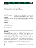
4.2 Precision and Recall Graphs
For a clearer picture, however, larger portions of
the SLs need to be examined. A well suited means
for comparing the goodness of different AMs are
the precision and recall graphs obtained by step-
wise processing of the complete SLs (Figures 1 to
10 below).
9
The
-axis represents the percentage of data
processed in the respective SL, while the
-

axis represents the precision (or recall) values
achieved. For instance, the precision values for
and for the AdjN data can be
read from the -axis in Figure 1 at positions where
and (marked by verti-
cal lines). The dotted horizontal line represents
the percentage of true collocations in the base set.
This value corresponds to the expected precision
value for random selection, and provides a base-
line for the interpretation of the precision curves.
General findings from the precision graphs are:
(i) It is only useful to consider the first halves
of the SLs, as the measures approximate after-
wards. (ii) Precision of log-likelihood, , t-test
and frequency strongly decreases in the first part
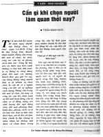
of the SLs, whereas precision of remains al-
most constant (cf. Figure 1) or even increases
slightly (cf. Figure 2). (iii) The identification re-
sults are instable for the first few percent of the
data, with log-likelihood, t-test and frequency sta-
bilizing earlier than and , and the PNV data
9
Colour versions of all plots in this paper will be avail-
able from />0% 10% 20% 30% 40% 50% 60% 70% 80% 90% 100%
0%
10%
20%
30%
40%
50%

60%
70%
part of significance list
precision
4652 candidates
frequency -test log-likelihood MI
Figure 1: Precision graphs for AdjN data.
0% 10% 20% 30% 40% 50% 60% 70% 80% 90% 100%
0%
10%
20%
30%
40%
50%
60%
part of significance list
precision
14654 candidates
frequency -test log-likelihood MI
Figure 2: Precision graphs for PNV data.
stabilizing earlier than the AdjN data. This in-
stability is caused by “random fluctuations”, i.e.,
whether a particular TP ends up on rank
(and
thus increases the precision of the -best list) or
on rank . The -best lists for AMs with low
precision values ( , ) contain a particularly
small number of TPs. Therefore, they are more
susceptible to random variation, which illustrates
that evaluation based on a small number of -best

candidate pairs cannot be reliable.
With respect to the recall curves (Figures 3 and
4), we find: (i) Examination of 50% of the data
in the SLs leads to identification of between 75%
(AdjN) and 80% (PNV) of the TPs. (ii) For the
first 40% of the SLs, and lead to the worst
results, with outperforming .
0% 10% 20% 30% 40% 50% 60% 70% 80% 90% 100%
0%
10%
20%
30%
40%
50%
60%
70%
80%
90%
100%
part of significance list
recall
4652 candidates
frequency -test log-likelihood MI
Figure 3: Recall graphs for AdjN data.
0% 10% 20% 30% 40% 50% 60% 70% 80% 90% 100%
0%
10%
20%
30%
40%

50%
60%
70%
80%
90%
100%
part of significance list
recall
14654 candidates
frequency -test log-likelihood MI
Figure 4: Recall graphs for PNV data.
Examining the precision and recall graphs in
more detail, we find that for the AdjN data (Fig-
ure 1), log-likelihood and t-test lead to the best re-
sults, with log-likelihood giving an overall better
result than the t-test. The picture differs slightly
for the PNV data (Figure 2). Here t-test outper-
forms log-likelihood, and even precision gained
by frequency is better than or at least comparable
to log-likelihood. These pairings – log-likelihood
and t-test for AdjN, and t-test and frequency for
PNV – are also visible in the recall curves (Fig-
ures 3 and 4). Moreover, for the PNV data the
t-test leads to a recall of over 60% when approx.
20% of the SL has been considered.
In the Figures above, there are a number of po-
sitions on the -axis where the precision and re-
call values of different measures are almost iden-
tical. This shows that a simple -best approach
will often produce misleading results. For in-

stance, if we just look at the first of
the SLs for the PNV data, we might conclude
that the t-test and frequency measures are equally
well suited for the extraction of PNV collocations.
However, the full curves in Figures 2 and 4 show
that t-test is consistently better than frequency.
4.3 Frequency Strata
While we have previously considered data from a
broad frequency range (i.e., frequencies
for AdjN and for PNV), we will now
split up the candidate sets into high-frequency and
low-frequency occurrences. This procedure al-
lows us to assess the performance of AMs within
different frequency strata. For instance, there is
a widely held belief that
and are inferior
to other measures because they overestimate the
collocativity of low-frequency candidates (cf. the
remarks on the measure in (Dunning, 1993)).
One might thus expect and to yield much
better results for higher frequencies.
We have divided the AdjN data into two sam-
ples with (high frequencies) and
(low frequencies), because the number of data
in the base sample is quite small. As there are
enough PNV data, we used a higher threshold and
selected samples with (high frequencies)
and (low frequencies).
High Frequencies
Considering our high-frequency AdjN data (Fig-

ure 5), we find that all precision curves decline as
more of the data in the SLs is examined. Espe-
cially for , this is markedly different from the
results obtained before. As the full curves show,
log-likelihood is obviously the best measure. It
is followed by t-test, , frequency and in
this order. Frequency and approximate when
50% of the data in the SLs are examined. In the
remaining part of the lists, yields better re-
sults than frequency and is practically identical to
the best-performing measures.
0% 10% 20% 30% 40% 50% 60% 70% 80% 90% 100%
0%
10%
20%
30%
40%
50%
60%
70%
part of significance list
precision
1280 candidates
frequency -test log-likelihood MI
Figure 5: AdjN data with
.
0% 10% 20% 30% 40% 50% 60% 70% 80% 90% 100%
0%
10%
20%

30%
40%
50%
60%
part of significance list
precision
1249 candidates
frequency -test log-likelihood MI
Figure 6: PNV data with
.
Surprisingly, the precision curves of and in
particular increase over the first 60% of the
SLs for high-frequency PNV data, whereas the
curves for t-test, log-likelihood, and frequency
have the usual downward slope (see Figure 6).
Log-likelihood achieves precision values above
50% for the first 10% of the list, but is outper-
formed by the t-test afterwards. Looking at the
first 40% of the data, there is a big gap between
the good measures (t-test, log-likelihood, and fre-
quency) and the weak measures ( and ).
In the second half of the data in the SLs, how-
ever, there is virtually no difference between ,
, and the other measures, with the exception of
mere co-occurrence frequency.
Summing up, t-test – with a few exceptions
around the first 5% of the data in the SLs –
leads to the overall best precision results for
high-frequency PNV data. Log-likelihood is sec-
ond best but achieves the best results for high-

frequency AdjN data.
Low Frequencies
0% 10% 20% 30% 40% 50% 60% 70% 80% 90% 100%
0%
10%
20%
30%
40%
part of significance list
precision
3372 candidates
frequency -test log-likelihood MI
Figure 7: AdjN data with
.
0% 10% 20% 30% 40% 50% 60% 70% 80% 90% 100%
0%
10%
part of significance list
precision
10165 candidates
frequency -test log-likelihood MI
Figure 8: PNV data with
.
Figures 7 and 8 show that there is little differ-
ence between the AMs for low-frequency data,
except for co-occurrence frequency, which leads
to worse results than all other measures.
For AdjN data, the AMs at best lead to an im-
provement of factor 3 compared to random selec-
tion (when up to of the SL is examined,

log-likelihood achieves precision values above
30%). Log-likelihood is the overall best measure
for identifying AdjN collocations, except for -
coordinates between 15% and 20% where t-test
outperforms log-likelihood.
For PNV data, the curves of all measures (ex-
cept for frequency) are nearly identical. Their
precision values are not significantly
10
different
from the baseline obtained by random selection.
In contrast to our expectation stated at the be-
ginning of this section, the performance of
and relative to the other AMs is not better for
high-frequency data than for low-frequency data.
Instead, the poor performance observed in section
4.2 is explained by the considerably higher base-
line precision of the high-frequency data (cf. Fig-
ures 5 to 8): unlike the -best lists for “frequency-
sensitive” measures such as log-likelihood, those
of and contain a large proportion of low-
frequency candidates.
5 Hapaxlegomena and Double
Occurrences
As the frequency distribution of word combina-
tions in texts is characterised by a large number
of rare events, low-frequency data are a serious
challenge for AMs. One way to deal with low-
frequency candidates is the introduction of cut-
off thresholds. This is a widely used strategy,

and it is motivated by the fact that it is in gen-
eral highly problematic to draw conclusions from
low-frequency data with statistical methods (cf.
Weeber et al. (2000) and Figure 8). A practical
reason for cutting off low-frequency data is the
need to reduce the amount of manual work when
the complete data set has to be evaluated, which
is a precondition for the exact calculation of recall
and for plotting precision curves.
The major drawback of an approach where all
low-frequency candidates are excluded is that a
large part of the data is lost for collocation extrac-
tion. In our data, for instance, 80% of the full set
of PNV data and 58% of the AdjN data are ha-
paxes. Thus it is important to know how many
(and which) true collocations there are among the
excluded low-frequency candidates.
5.1 Statistical Estimation of TPs among
Low-Frequency Data
In this section, we estimate the number of col-
locations in the data excluded from our experi-
ments (i.e., AdjN pairs with
and PNV
triples with ). Because of the large num-
ber of candidates in those sets (6 435 for AdjN,
10
According to the -test as described in section 6.
279 880 for PNV), manual inspection of the en-
tire data is impractical. Therefore, we use ran-
dom samples from the candidate sets to obtain es-

timates for the proportion of true collocations
among the low-frequency data. We randomly se-
lected 965 items (15%) from the AdjN hapaxes,
and 983 items (
0.35%) from the low-frequency
PNV triples. Manual examination of the samples
yielded 31 TPs for AdjN (a proportion of 3.2%)
and 6 TPs for PNV (0.6%).
Considering the low proportion of collocations
in the samples, we must expect highly skewed
frequency distributions (where is very small),
which are problematic for standard statistical
tests. In order to obtain reliable estimates, we
have used an exact test based on the following
model: Assuming a proportion of TPs in the full
low-frequency data (AdjN or PNV), the number
of TPs in a random sample of size
is described
by a binomially distributed random variable
with parameter .
11
Consequently, the proba-
bility of finding or less TPs in the sample is
. We ap-
ply a one-tailed statistical test based on the proba-
bilities to our samples in order to ob-
tain an upper estimate for the actual proportion of
collocations among the low-frequency data: the
estimate is accepted at a given signifi-
cance level if .

In the case of the AdjN data ( ,
), we find that at a confidence level of
99% ( ). Thus, there should be at most
320 TPs among the AdjN candidates with .
Compared to the 737 TPs identified in the AdjN
data with , our decision to exclude the ha-
paxlegomena was well justified. The proportion
of TPs in the PNV sample ( , )
was much lower and we find that at
the same confidence level of 99%. However, due
to the very large number of low-frequency candi-
dates, there may be as many as 4200 collocations
in the PNV data with , more than 4 times
the number identified in our experiment.
It is imaginable, then, that one of the AMs
11
To be precise, the binomial distribution is itself an ap-
proximation of the exact hypergeometric probabilities (cf.
Pedersen (1996)). This approximation is sufficiently accu-
rate as long as the sample size
is small compared to the
size of the base set (i.e., the number of low-frequency candi-
dates).
0% 10% 20% 30% 40% 50% 60% 70% 80% 90% 100%
0%
10%
part of significance list
precision
10000 candidates
frequency -test log-likelihood MI

Figure 9: PNV data with
.
might succeed in extracting a substantial num-
ber of collocations from the low-frequency PNV
data. Figure 9 shows precision curves for the
10 000 highest ranked word combinations from
each SL for PNV combinations with
(the vertical lines correspond to -best lists for
).
In order to reduce the amount of manual work,
the precision values for each AM are based on
a 10% random sample from the 10 000 highest
ranked candidates. We have applied the statisti-
cal test described above to obtain confidence in-
tervals for the true precision values of the best-
performing AM (frequency), given our 10% sam-
ple. The upper and lower bounds of the 95% con-
fidence intervals are shown as thin lines. Even
the highest precision estimates fall well below the
6.41% precision baseline of the PNV data with
. Again, we conclude that the exclusion of
low-frequency candidates was well justified.
6 Significance Testing
We have assessed the significance of differences
between AMs using the well-known test as de-
scribed in (Krenn, 2000).
12
The thin lines in Fig-
ure 10 delimit 95% confidence intervals around
the best-performing measure for the AdjN data

with (log-likelihood).
There is no significant difference between log-
likelihood and t-test. And only for -best lists
with , frequency performs marginally
significantly worse than log-likelihood. For the
PNV data (not shown), the t-test is signifi-
cantly better than log-likelihood, but the differ-
ence between frequency and the t-test is at best
marginally significant.
12
See (Krenn and Evert, 2001) for a short discussion of
the applicability of this test.
0% 10% 20% 30% 40% 50% 60% 70% 80% 90% 100%
0%
10%
20%
30%
40%
50%
60%
70%
part of significance list
precision
4652 candidates
frequency -test log-likelihood MI
Figure 10: Significance of differences (AdjN)
7 Conclusion
We have shown that simple
-best approaches are
not suitable for a qualitative evaluation of lexi-

cal association measures, mainly for the follow-
ing reasons: the instability of precision values ob-
tained from the first few percent of the data in the
SLs; the lack of significant differences between
the AMs after approx. 50% of the data in the SLs
have been examined; and the lack of significant
differences between the measures except for cer-
tain specific values of
. We have also shown that
the evaluation results and the ranking of AMs dif-
fer depending on the kind of collocations to be
identified, and the proportion of hapaxes in the
candidate sets. Finally, our results question the
widely accepted argument that the strength of log-
likelihood lies in handling low-frequency data. In
our experiments, none of the AMs was able to ex-
tract a substantial number of collocations from the
set of hapaxlegomena.
Acknowledgement
The work of B. Krenn has been sponsored by
the Fonds zur Förderung der wissenschaftlichen
Forschung (FWF), Grant No. P12920. Financial
support for ÖFAI is provided by the Austrian Fed-
eral Ministry of Education, Science and Culture.
The AdjN data is the result of joint research with
Ulrich Heid and Wolfgang Lezius.
The authors would like to thank the anonymous
reviewers for many helpful comments and inter-
esting references.
References

Hadumod Bußmann. 1990. Lexikon der Sprachwis-
senschaft. Kröner, 2nd edition.
K.W. Church and P. Hanks. 1989. Word association
norms, mutual information, and lexicography. In
Proceedings of the 27th Annual Meeting of the As-
sociation for Computational Linguistics, Vancou-
ver, Canada, 76–83.
Ted Dunning. 1993. Accurate methods for the statis-
tics of surprise and coincidence. Computational
Linguistics, 19(1):61–74.
Stefan Evert, Ulrich Heid, and Wolfgang Lezius.
2000. Methoden zum Vergleich von Signifikanz-
maßen zur Kollokationsidentifikation. In Proceed-
ings of KONVENS 2000, VDE-Verlag, Germany,
pages 215 – 220.
Adam Kilgarriff. 1996. Which words are particularly
characteristic of a text? A survey of statistical ap-
proaches. In Proceedings of the AISB Workshop on
Language Engineering for Document Analysis and
Recognition, Sussex University, GB.
Brigitte Krenn. 2000. The Usual Suspects: Data-
Oriented Models for the Identification and Repre-
sentation of Lexical Collocations. DFKI & Univer-
sität des Saarlandes, Saarbrücken.
Brigitte Krenn and Stefan Evert. 2001. Can we do
better than frequency? A case study on extracting
PP-verb collocations. In Proceedings of the ACL
Workshop on Collocations, Toulouse, France.
Wolfgang Lezius. 1999. Automatische Extrahierung
idiomatischer Bigramme aus Textkorpora. In

Tagungsband des 34. Linguistischen Kolloquiums,
Germersheim.
Christopher D. Manning and Hinrich Schütze. 1999.
Foundations of Statistical Natural Language Pro-
cessing. MIT Press, Cambridge, MA.
Ted Pedersen. 1996. Fishing for Exactness. In Pro-
ceedings of the South-Central SAS Users Group
Conference, Austin, TX.
Helmut Schmid. 1995. Improvements in part-of-
speech tagging with an application to german. In
Proceedings of the ACL SIGDAT-Workshop, 47–50.
Wojciech Skut and Thorsten Brants. 1998. Chunk
Tagger. Stochastic Recognition of Noun Phrases. In
ESSLI Workshop on Automated Acquisition of Syn-
tax and Parsing, Saarbrücken, Germany.
Mark Weeber, Rein Vos, and Harald R. Baayen 2000.
Extracting the lowest-frequency words: Pitfalls and
possibilities. Computational Linguistics, 26(3).