Tài liệu Báo cáo khoa học: "Distributional Similarity Models: Clustering Neighbors" doc

Distributional Similarity Models: Clustering
vs.
Nearest
Neighbors
Lillian
Lee
Department of Computer Science
Cornell University
Ithaca, NY 14853-7501
llee@cs, cornell, edu
Fernando Pereira
A247, AT&T Labs - Research
180 Park Avenue
Florham Park, NJ 07932-0971
pereira@research, att.
com
Abstract
Distributional similarity is a useful notion in es-
timating the probabilities of rare joint events.
It has been employed both to cluster events ac-
cording to their distributions, and to directly
compute averages of estimates for distributional
neighbors of a target event. Here, we examine
the tradeoffs between model size and prediction
accuracy for cluster-based and nearest neigh-
bors distributional models of unseen events.
1
Introduction
In many statistical language-processing prob-
lems, it is necessary to estimate the joint proba-
bility or

cooeeurrence probability
of events drawn
from two prescribed sets. Data sparseness can
make such estimates difficult when the events
under consideration are sufficiently fine-grained,
for instance, when they correspond to occur-
rences of specific words in given configurations.
In particular, in many practical modeling tasks,
a substantial fraction of the cooccurrences of in-
terest have never been seen in training data. In
most previous work (Jelinek and Mercer, 1980;
Katz, 1987; Church and Gale, 1991; Ney and
Essen, 1993), this lack of information is ad-
dressed by reserving some mass in the proba-
bility model for unseen joint events, and then
assigning that mass to those events as a func-
tion of their marginal frequencies.
An intuitively appealing alternative to relying
on marginal frequencies alone is to combine es-
timates of the probabilities of "similar" events.
More specifically, a joint event (x, y) would be
considered similar to another (x t, y) if the distri-
butions of Y given x and Y given x' (the cooc-
currence distributions of x and x ') meet an ap-
propriate definition of distributional similarity.
For example, one can infer that the bigram "af-
ter ACL-99" is plausible even if it has never
33
occurred before from the fact that the bigram
"after ACL-95"

has
occurred, if "ACL-99" and
"ACL-95" have similar cooccurrence distribu-
tions.
For concreteness and experimental evalua-
tion, we focus in this paper on a particular type
of cooccurrence, that of a main verb and the
head noun of its direct object in English text.
Our main goal is to obtain estimates
~(vln )
of
the conditional probability of a main verb v
given a direct object head noun n, which can
then be used in particular prediction tasks.
In previous work, we and our co-authors have
proposed two different probability estimation
methods that incorporate word similarity infor-
mation: distributional clustering and nearest-
neighbors averaging.
Distributional clustering
(Pereira et al., 1993) assigns to each word a
probability distribution over clusters to which
it may belong, and characterizes each cluster
by a
centroid,
which is an average of cooccur-
rence distributions of words weighted according
to cluster membership probabilities. Cooccur-
rence probabilities can then be derived from ei-
ther a membership-weighted average of the clus-

ters to which the words in the cooccurrence be-
long, or just from the highest-probability clus-
ter.
In contrast,
nearest-neighbors averaging 1
(Dagan et al., 1999) does not explicitly clus-
ter words. Rather, a given cooccurrence prob-
ability is estimated by averaging probabilities
for the set of cooccurrences most similar to the
target cooccurrence. That is, while both meth-
ods involve appealing to similar "witnesses" (in
the clustering case, these witnesses are the cen-
troids; for nearest-neighbors averaging, they are
1In previous papers, we have used the term
"similarity-based", but this term would cause confusion
in the present article.
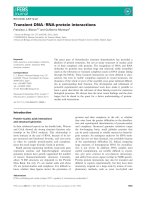
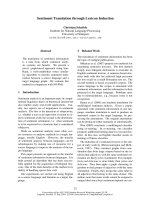
the most similar words), in nearest-neighbors
averaging the witnesses vary for different cooc-
currences, whereas in distributional clustering
the same set of witnesses is used for every cooc-
currence (see Figure 1).
We thus see that distributional clustering and
nearest-neighbors averaging are complementary
approaches. Distributional clustering gener-
ally creates a compact representation of the
data, namely, the cluster membership probabil-
ity tables and the cluster centroids. Nearest-
neighbors averaging, on the other hand, asso-
ciates a specific set of similar words to each word
and thus typically increases the amount of stor-

age required. In a way, it is clustering taken to
the limit - each word forms its own cluster.
In previous work, we have shown that both
distributional clustering and nearest-neighbors
averaging can yield improvements of up to 40%
with respect to Katz's (1987) state-of-the-art
backoffmethod
in the prediction of unseen cooc-
currences. In the case of nearest-neighbors aver-
aging, we have also demonstrated perplexity re-
ductions of 20% and statistically significant im-
provement in speech recognition error rate. Fur-
thermore, each method has generated some dis-
cussion in the literature (Hofmann et al., 1999;
Baker and McCallum, 1998; Ide and Veronis,
1998). Given the relative success of these meth-
ods and their complementarity, it is natural to
wonder how they compare in practice.
Several authors (Schiitze, 1993; Dagan et al.,
1995; Ide and Veronis, 1998) have suggested
that clustering methods, by reducing data to
a small set of representatives, might perform
less well than nearest-neighbors averaging-type
methods. For instance, Dagan et al. (1995,
p. 124) argue:
This [class-based] approach, which fol-
lows long traditions in semantic clas-
sification, is very appealing, as it at-
tempts to capture "typical" properties
of classes of words. However it is

not clear that word co-occurrence pat-
terns can be generalized to class co-
occurrence parameters without losing
too much information.
Furthermore, early work on class-based lan-
guage models was inconclusive (Brown et al.,
1992).
34
In this paper, we present a detailed com-
parison of distributional clustering and nearest-
neighbors averaging on several large datasets,
exploring the tradeoff in similarity-based mod-
eling between memory usage on the one hand
and estimation accuracy on the other. We find
that the performances of the two methods are
in general very similar: with respect to Katz's
back-off, they both provide average error reduc-
tions of up to 40% on one task and up to 7%
on a related, but somewhat more difficult, task.
Only in a fairly unrealistic setting did nearest-
neighbors averaging clearly beat distributional
clustering, but even in this case, both meth-
ods were able to achieve average error reduc-
tions of at least 18% in comparison to back-
off. Therefore, previous claims that clustering
methods are necessarily inferior are not strongly
supported by the evidence of these experiments,
although it is of course possible that the situa-
tion may be different for other tasks.
2 Two models

We now survey the distributional clustering
(section 2.1) and nearest-neighbors averaging
(section 2.2) models. Section 2.3 examines the
relationships between these two methods.
2.1 Clustering
The distributional clustering model that we
evaluate in this paper is a refinement of our ear-
lier model (Pereira et al., 1993). The new model
has important theoretical advantages over the
earlier one and interesting mathematical prop-
erties, which will be discussed elsewhere. Here,
we will outline the main motivation for the
model, the iterative equations that implement
it, and their practical use in clustering.
The model involves two discreterandom vari-
ables N (nouns) and V (verbs) whose joint dis-
tribution we have sampled, and a new unob-
served discrete random variable C representing
probabilistic clusters of elements of N. The
role of the hidden variable C is specified by
the conditional distribution
p(cln),
which can
be thought of as the probability that n belongs
to cluster c. We want to preserve in C as much
as possible of the information that N has about
V, that is, maximize the mutual information 2
I(V, C).
On the other hand, we would also
2I( X, Y) = ~-]~x ~ P(x, y)

log
(P(x, y)/P(x)P(y)).
6" ""
"o
o",0
I
I I I ~' ~ O s /
',,
O A O B
___
Figure 1: Difference between clustering and nearest neighbors. Although A and B belong mostly to
the same cluster (dotted ellipse), the two nearest neighbors to A are
not
the nearest two neighbors
to B.
like to control the degree of compression of C
relative to N, that is, the mutual information
I(C,N).
Furthermore, since C is intended to
summarize N in its role as a predictor of V, it
should carry no information about V that N
does not already have. That is, V should be
conditionally independent of C given N, which
allows us to write
p(vlc ) = ~-]p(vln)p(nlc ) .
(1)
n
The distribution
p(VIc )
is the

centroid
for clus-
ter c.
It can be shown that
I(V, C)
is maximized
subject to fixed
I(C, N)
and the above condi-
tional independence assumption when
p(c)
p(cln )
= ~ exp
[-/3D(p(Yln)]]p(Ylc) ) ] ,
(2)
where /3 is the Lagrange multiplier associated
with fixed
I(C,
N),
Zn
is the normalization
Zn = y~ p(c)
exp
[-/3D(p(Y[n)llp(Ylc ))]
,
c
and D is the
KuUback-Leiber (KL) divergence,
which measures the distance, in an information-
theoretic sense, between two distributions q and

r:
• q(v)
D(qllr ) = ~ q(v) lOgr(v) .
v
The main behavioral difference between this
model and our previous one is the
p(c)
factor in
(2), which tends to sharpen cluster membership
distributions. In addition, our earlier experi-
ments used a uniform marginal distribution for
the nouns instead of the marginal distribution
in the actual data, in order to make clustering
more sensitive to informative but relatively rare
35
nouns. While neither difference leads to major
changes in clustering results, we prefer the cur-
rent model for its better theoretical foundation.
For fixed /3, equations (2) and (1) together
with Bayes rule and marginalization can be used
in a provably convergent iterative reestimation
process for
p(glc), p(YlC )
and
p(C).
These
distributions form the
model
for the given/3.
It is easy to see that for/3 = 0,

p(nlc )
does not
depend on the cluster distribution
p(VIc),
so the
natural number of clusters (distinct values of
C) is one. At the other extreme, for very large
/3 the natural number of clusters is the same
as the number of nouns. In general, a higher
value of/3 corresponds to a larger number of
clusters. The natural number of clusters k and
the probabilistic model for different values of/3
are estimated as follows. We specify an increas-
ing sequence {/3i} of/3 values (the "annealing"
schedule), starting with a very low value/30 and
increasing slowly (in our experiments, /30 = 1
and/3i+1 = 1-1/30. Assuming that the natural
number of clusters and model for/3i have been
computed, we set/3 =/3i+1 and split each clus-
ter into two
twins
by taking small random per-
turbations of the original cluster centroids. We
then apply the iterative reestimation procedure
until convergence. If two twins end up with sig-
nificantly different centroids, we conclude that
they are now separate clusters. Thus, for each
i we have a number of clusters ki and a model
relating those clusters to the data variables N
and V.

A cluster model can be used to estimate
p(vln )
when v and n have not occurred together
in training. We consider two heuristic ways of
doing this estimation:
• all-cluster
weighted average:
p(vln) =
~-]p(vlc)p(cln)
c
• nearest-cluster
estimate:
~(vln)
p(vlc*),
where c* maximizes
p(c*ln).
2.2 Nearest-neighbors averaging
As noted earlier, the nearest-neighbors averag-
ing method is an alternative to clustering for
estimating the probabilities of unseen cooccur-
fences. Given an unseen pair (n, v), we calcu-
late
an estimate 15(vln ) as an appropriate aver-
age of
p(vln I)
where n I is distributionally sim-
ilar to n. Many distributional similarity mea-
sures can be considered (Lee, 1999). In this
paper, we focus on the one that gave the best
results in our earlier work (Dagan et al., 1999),

the
Jensen-Shannon divergence
(Rao, 1982; Lin,
1991). The Jensen-Shannon divergence of two
discrete distributions p and q over the same do-
main is defined as
1
gS(p, q) = ~
It is easy to see that
JS(p, q)
is always defined.
In previous work, we used the estimate
~5(vln ) = 1 ~
p(vln,)exp(_Zj(n,n,)),
(In nlES(n,k)
where
J(n,n') = JS (p(VIn),p(Yln')), Z
and
k are tunable parameters,
S(n, k)
is the set of
k nouns with the smallest Jensen-Shannon di-
vergence to n, and an is a normalization term.
However, in the present work we use the simpler
unweighted average
1
/~(vln)
= -~ ~ p(vln'),
(3)
n'ES(n,k)

and examine the effect of the choice of k on
modeling performance. By eliminating extra
parameters, this restricted formulation allows a
more direct comparison of nearest-neighbors av-
eraging to distributional clustering, as discussed
in the next section. Furthermore, our earlier
experiments showed that an exponentially de-
creasing weight has much the same effect on per-
formance as a bound on the number of nearest
neighbors participating in the estimate.
2.3 Discussion
In the previous two sections, we presented
two complementary paradigms for incorporat-
ing distributional similarity information into
cooccurrence probability estimates. Now, one
cannot always draw conclusions about the rel-
ative fitness of two methods simply from head-
to-head performance comparisons; for instance,
one method might actually make use of inher-
ently more informative statistics but produce
worse results because the authors chose a sub-
optimal weighting scheme. In the present case,
however, we are working with two models which,
while representing opposite extremes in terms of
generalization, share enough features to make
the comparison meaningful.
First, both models use linear combinations
of cooccurrence probabilities for similar enti-
ties. Second, each has a single free param-
eter k, and the two k's enjoy a natural in-

verse correspondence: a large number of clus-
ters in the distributional clustering case results
in only the closest centroids contributing sig-
nificantly to the cooccurrence probability esti-
mate, whereas a large number of neighbors in
the nearest-neighbors averaging case means that
relatively distant words are consulted. And fi-
nally, the two distance functions are similar in
spirit: both are based on the KL divergence to
some type of averaged distribution. We have
thus attempted to eliminate functional form,
number and type of parameters, and choice of
distance function from playing a role in the com-
parison, increasing our confidence that we are
truly comparing paradigms and not implemen-
tation details.
What are the fundamental differences be-
tween the two methods? From the foregoing
discussion it is clear that distributional clus-
tering is theoretically more satisfying and de-
pends on a single model complexity parameter.
On the other hand, nearest-neighbors averaging
in its most general form offers more flexibility
in defining the set of most similar words and
their relative weights (Dagan et al., 1999). Also,
the training phase requires little computation,
as opposed to the iterative re-estimation proce-
dure employed to build the cluster model. But
the key difference is the amount of data com-
pression, or equivalently the amount of general-

ization, produced by the two models. Cluster-
3{}
ing yields a far more compact representation of
the data when k, the model size parameter, is
smaller than INf. As noted above, various au-
thors have conjectured that this data reduction
must inevitably result in lower performance in
comparison to nearest-neighbor methods, which
store the most specific information for each in-
dividual word. Our experiments aim to ex-
plore this hypothesized generalization-accuracy
tradeoff.
3 Evaluation
3.1 Methodology
We compared the two similarity-based esti-
mation techniques at the following decision
task, which evaluates their ability to choose
the more likely of two unseen cooccurrences.
Test instances consist of noun-verb-verb triples
(n, vl, v2), where both (n, Vl) and (n, v2) are un-
seen cooccurrences, but (n, vl) is more likely
(how this is determined is discussed below). For
each test instance, the language model prob-
abilities 151
dej
15(vlln)
and i52
dej
15(v2]n) are
computed; the result of the test is either cor-

rect (151 > 152), incorrect (/51 < ~52,) or a tie
(151 = 152). Overall performance is measured by
the error rate on the entire test set, defined as
1
~(# of incorrect choices + (# of ties)/2),
where T is the number of test triples, not count-
ing multiplicities.
Our global experimental design was to run
ten-fold cross-validation experiments comparing
distributional clustering, nearest-neighbors av-
eraging, and Katz's backoff (the baseline) on the
decision task just outlined. All results we report
below are averages over the ten train-test splits.
For each split, test triples were created from the
held-out test set. Each model used the training
set to calculate all basic quantities (e.g.,
p(vln )
for each verb and noun), but
not
to train k.
Then, the performance of each similarity-based
model was evaluated on the test triples for a
sequence of settings for k.
We expected that clustering performance
with respect to the baseline would initially im-
prove and then decline. That is, we conjec-
tured that the model would overgeneralize at
small k but overfit the training data at large
k. In contrast, for nearest-neighbors averag-
ing, we hypothesized monotonically decreasing

performance curves: using only the very most
similar words would yield high performance,
whereas including more distant, uninformative
words would result in lower accuracy. From pre-
vious experience, we believed that both meth-
ods would do well with respect to backoff.
3.2 Data
In order to implement the experimental
methodology just described, we employed the
follow
data
preparation method:
i. Gather verb-object pairs using the CASS
partial parser (Abney, 1996)
Partition set of pairs into ten folds
.
3.
For each test fold,
(a) discard seen pairs and duplicates
(b) discard pairs with unseen nouns or un-
seen verbs
(e) for each remaining (n, vl), create
(n, vl, v2) such that (n, v~) is less likely
Step 3b is necessary because neither the
similarity-based methods nor backoff handle
novel unigrams gracefully.
We instantiated this schema in three ways:
AP89 We retrieved 1,577,582 verb-object
pairs from 1989 Associated Press (AP)
newswire, discarding singletons (pairs occurring

only once) as is commonly done in language
modeling. We split this set by type 3, which
does not realistically model how new data oc-
curs in real life, but does conveniently guaran-
tee that the entire test set is unseen. In step
3c all (n, v2) were found such that (n, vl) oc-
curred at least twice as often as (n, v2) in the
test fold; this gives reasonable reassurance that
n is indeed more likely to cooccur with Vl, even
though (n, v2) is plausible (since it did in fact
occur).
3When a corpus is split by
type,
all instances of a
given type must end up in the same partition. If the
split is by
token,
then instances of the same type may
end up in different partitions. For example, for corpus
'% b a c', "a b" +"a c" is a valid split by token, but not
by type.
37
Test type
AP89
AP90unseen
AP90fake
split singletons? ~ training
%
of test ~ test baseline
pairs unseen triples error

type no 1033870 100 42795 28.3%
token yes 1123686 14 4019 39.6%
" " " " 14479 79.9%
Table 1: Data for the three types of experiments. All numbers are averages over the ten splits.
AP90unseen 1,483,728 pairs were extracted
from 1990 AP newswire and split by token. Al-
though splitting by token is undoubtedly a bet-
ter way to generate train-test splits than split-
ting by type, it had the unfortunate side effect
of diminishing the average percentage of unseen
cooccurrences in the test sets to 14%. While
this is still a substantial fraction of the data
(demonstrating the seriousness of the sparse
data problem), it caused difficulties in creat-
ing test triples: after applying filtering step 3b,
there were relatively few candidate nouns and
verbs satisfying the fairly stringent condition 3c.
Therefore, singletons were retained in the AP90
data. Step 3c was carried out as for AP89.
AP90fake The procedure for creating the
AP90unseen data resulted in much smaller test
sets than in the AP89 case (see Table I). To
generate larger test sets, we used the same folds
as in AP90unseen, but implemented step 3c dif-
ferently. Instead of selecting v2 from cooccur-
rences (n, v2) in the held-out set, test triples
were constructed using v2 that never cooccurred
with n in either the training or the test data.
That is, each test triple represented a choice
between a plausible cooccurrence (n, Vl) and an

implausible ("fake") cooccurrence (n, v2). To
ensure a large differential between the two al-
ternatives, we further restricted (n, Vl) to occur
at least twice (in the test fold). We also chose v2
from the set of 50 most frequent verbs, resulting
in much higher error rates for backoff.
3.3 Results
We now present evaluation results ordered by
relative difficulty of the decision task.
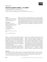
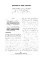
Figure 2 shows the performance of distribu-
tional clustering and nearest-neighbors averag-
ing on the AP90fake data (in all plots, error bars
represent one standard deviation). Recall that
the task here was to distinguish between plau-
sible and implausible cooccurrences, making it
38
a somewhat easier problem than that posed in
the AP89 and AP90unseen experiments. Both
similarity-based methods improved on the base-
line error (which, by construction of the test
triples, was guaranteed to be high) by as much
as 40%. Also, the curves have the shapes pre-
dicted in section 3.1.
all
clu'sters
nearest cluster
5'0 ,~0 ,~0 2~0 2;0
~0 g0 ,~
k
Figure 2: Average error reduction with respect

to backoff on AP90fake test sets.
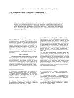
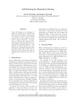
We next examine our AP89 experiment re-
sults, shown in Figure 3. The similarity-based
methods clearly outperform backoff, with the
best error reductions occurring at small k for
both types of models. Nearest-neighbors aver-
aging appears to have the advantage over dis-
tributional clustering, and the nearest cluster
method yields lower error rates than the aver-
aged cluster method (the differences are statisti-
cally significant according to the paired t-test).
We might hypothesize that nearest-neighbors
averaging is better in situations of extreme spar-
sity of data. However, these results must be
taken with some caution given their unrealistic
type-based train-test split.
A striking feature of Figure 3 is that all the
curves have the same shape, which is not at all
what we predicted in section 3.1. The reason
]
10
all clusters
nearest cluster
nearest neighbors
25
o , , , , , ,
5 100 150 200 250 300 350 400
k
Figure 3: Average error reduction with respect
to backoff on AP89 test sets.

0.26
0.26
0.24
0.23
0.22
0.21
0.2
0.1~
that the very most similar words are appar-
ently not as informative as slightly more dis-
tant words is due to recall errors. Observe that
if (n, vl) and (n, v2) are unseen in the train-
ing data, and if word n' has very small Jensen-
Shannon divergence to n, then chances are that
n ~ also does not occur with either Vl or v2, re-
sulting in an estimate of zero probability for
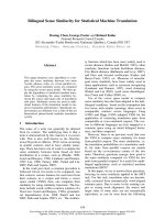
both test cooccurrences. Figure 4 proves that
this is the case: if zero-ties are ignored, then the
error rate curve for nearest-neighbors averaging
has the expected shape. Of course, clustering is
not prone to this problem because it automati-
cally smoothes its probability estimates.
average error over APe9, normal vs. precision results
nearest neighbors
nearest neighbors. Ignodng recall errors
•'0
' ' ' ' ' '
100 150 200 250 300 350 400
k
Figure 4: Average error (not error reduction)

using nearest-neighbors averaging on AP89,
showing the effect of ignoring recall mistakes.
Finally, Figure 5 presents the results of
39
our AP90unseen experiments. Again, the use
of similarity information provides better-than-
baseline performance, but, due to the relative
difficulty of the decision task in these exper-
iments (indicated by the higher baseline er-
ror rate with respect to AP89), the maximum
average improvements are in the 6-8% range.
The error rate reductions posted by weighted-
average clustering, nearest-centroid clustering,
and nearest-neighbors averaging are all well
within the standard deviations of each other.
I
all clusters
nearest cluster
nearest neighbors
-2
0 50 100 150 200 250 300 350 400
k
Figure 5: Average error reduction with respect
to backoff on AP90unseen test sets. As in the
AP89 case, the nonmonotonicity of the nearest-
neighbors averaging curve is due to recall errors.
4 Conclusion
In our experiments, the performances of distri-
butional clustering and nearest-neighbors aver-
aging proved to be in general very similar: only

in the unorthodox AP89 setting did nearest-
neighbors averaging clearly yield better error
rates. Overall, both methods achieved peak per-
formances at relatively small values of k, which
is gratifying from a computational point of view.
Some questions remain. We observe that
distributional clustering seems to suffer higher
variance. It is not clear whether this is due
to poor estimates of the KL divergence to cen-
troids, and thus cluster membership, for rare
nouns, or to noise sensitivity in the search for
cluster splits. Also, weighted-average clustering
never seems to outperform the nearest-centroid
method, suggesting that the advantages of prob-
abilistic clustering over "hard" clustering may
be computational rather than in modeling el-
fectiveness (Boolean clustering is NP-complete
(Brucker, 1978)). Last but not least, we do not
yet have a principled explanation for the similar
performance of nearest-neighbors averaging and
distributional clustering. Further experiments,
especially in other tasks such as language mod-
eling, might help tease apart the two methods
or better understand the reasons for their simi-
larity.
5 Acknowledgements
We thank the anonymous reviewers for their
helpful comments and Steve Abney for help
with extracting verb-object pairs with his parser
CASS.

References
Steven Abney. 1996. Partial parsing via finite-state
cascades. In
Proceedings of the ESSLLI '96 Ro-
bust 15arsing Workshop.
L. Douglas Baker and Andrew Kachites McCallum.
1998. Distributional clustering of words for text
classification. In
Plst Annual International A CM
SIGIR Conference on Research and Development
in Information Retrieval (SIGIR '98),
pages 96-
103.
Peter F. Brown, Vincent J. DellaPietra, Peter V.
deSouza, Jennifer C. Lai, and Robert L. Mercer.
1992. Class-based n-gram models of natural lan-
guage.
Computational Linguistics,
18(4):467-479,
December.
Peter Brucker. 1978. On the complexity of clus-
tering problems. In Rudolf Henn, Bernhard H.
Korte, and Werner Oettli, editors,
Optimization
and Operations Research,
number 157 in Lecture
Notes in Economics and Mathematical Systems.
Springer-Verlag, Berlin.
Kenneth W. Church and William A. Gale. 1991.
A comparison of the enhanced Good-Turing and

deleted estimation methods for estimating proba-
bilities of English bigrams.
Computer Speech and
Language,
5:19-54.
Ido Dagan, Shaul Marcus, and Shaul Markovitch.
1995. Contextual word similarity and estimation
from sparse data.
Computer Speech and Lan-
guage,
9:123-152.
Ido Dagan, Lillian Lee, and Fernando Pereira. 1999.
Similarity-based models of word cooccurrence
probabilities.
Machine Learning,
34(1-3):43-69.
Thomas Hofmann, Jan Puzicha, and Michael I. Jor-
dan. 1999. Learning from dyadic data. In
Ad-
vances in Neural Information Processing Systems
11.
MIT Press. To appear.
Nancy Ide and Jean Veronis. 1998. Introduction to
the special issue on word sense disambiguation:
40
The state of the art.
Computational Linguistics,
24(1):1-40, March.
Frederick Jelinek and Robert L. Mercer. 1980. Inter-
polated estimation of Markov source parameters

from sparse data. In
Proceedings of the Workshop
on Pattern Recognition in Practice,
Amsterdam,
May. North Holland.
Slava M. Katz. 1987. Estimation of probabilities
from sparse data for the language model com-
ponent of a speech recognizer.
IEEE Transac-
tions on Acoustics, Speech and Signal Processing,
ASSP-35(3):400-401, March.
Lillian Lee. 1999. Measures of distributional simi-
larity. In
37th Annual Meeting of the ACL,
Som-
erset, New Jersey. Distributed by Morgan Kauf-
mann, San Francisco.
Jianhua Lin. 1991. Divergence measures based on
the Shannon entropy.
IEEE Transactions on In-
formation Theory,
37(1):145-151.
Hermann Ney and Ute Essen. 1993. Estimating
'small' probabilities by leaving-one-out. In
Third
European Conference On Speech Communication
and Technology,
pages 2239-2242, Berlin, Ger-
many.
Fernando C. N. Pereira, Naftali Tishby, and Lillian

Lee. 1993. Distributional clustering of English
words. In
31st Annual Meeting of the ACL,
pages
183-190, Somerset, New Jersey. Association for
Computational Linguistics. Distributed by Mor-
gan Kaufmann, San Francisco.
C. Radhakrishna Rao. 1982. Diversity: Its measure-
ment, decomposition, apportionment and analy-
sis.
SankyhS: The Indian Journal of Statistics,
44(A):1-22.
Hinrich Schiitze. 1993. Word space. In S. J. Hanson,
J. D. Cowan, and C. L. Giles, editors,
Advances in
Neural Information Processing Systems 5,
pages
895-902. Morgan Kaufmann, San Francisco.