J a bergstra, a ponse, s a smolka handbook of process algebra elsevier science (2001)
Bạn đang xem bản rút gọn của tài liệu. Xem và tải ngay bản đầy đủ của tài liệu tại đây (47.44 MB, 1,328 trang )
Preface
1. Introduction
According to the Oxford English Dictionary (OED II CD-ROM), a process is a series of
actions or events, and an algebra is a calculus of symbols combining according to certain
defined laws. Completing the picture, a calculus is a system or method of calculation.
Despite going back as far as the 13th Century, collectively, these definitions do a good job
of accurately conveying the meaning of this Handbook's subject: process algebra.
A process algebra is a formal description technique for complex computer systems, especially those with communicating, concurrently executing components. A number of different process algebras have been developed - ACP [1], CCS [6], and TCSP [2] being
perhaps the best-known - but all share the following key ingredients.
• Compositional modeling. Process algebras provide a small number of constructs for
building larger systems up from smaller ones. CCS, for example, contains six operators
in total, including ones for composing systems in parallel and others for choice and
scoping.
• Operational semantics. Process algebras are typically equipped with a Plotkin-style [7]
structural operational semantics (SOS) that describes the single-step execution capabilities of systems. Using SOS, systems represented as terms in the algebra can be "compiled" into labeled transition systems.
• Behavioral reasoning via equivalences and preorders. Process algebras also feature
the use of behavioral relations as a means for relating different systems given in the
algebra. These relations are usually equivalences, which capture a notion of ''same behavior", or preorders, which capture notions of ''refinement".
In a process-algebraic approach to system verification, one typically writes two specifications. One, call it SYS, captures the design of the actual system and the other, call it
SPEC, describes the system's desired "high-level" behavior. One may then establish the
correctness of SYS with respect to SPEC by showing that SYS behaves the "same as" SPEC
(if using an equivalence) or by showing that it refines SPEC (if using a preorder).
Establishing the correctness of SYS with respect to SPEC can be done in a syntaxoriented manner or in a semantics-oriented manner. In the former case, an axiomatization
of the behavioral relation of choice is used to show that one expression can be transformed
into the other via syntactic manipulations. In the latter case, one can appeal directly to
the definition of the behavioral relation, and to the operational semantics of the two expressions, to show that they are related. In certain cases, e.g., when SYS and SPEC are
"finite-state", verification, be it syntax-based or semantics-based, can be carried out automatically.
vi
Preface
The advantages to an algebraic approach are the following.
• System designers need learn only one language for specifications and designs.
• Related processes may be substituted for one another inside other processes. This
makes process algebras particularly suitable for the modular analysis of complex systems, since a specification and a design adhering to this specification may be used interchangeably inside larger systems.
• Processes may be minimized with respect to the equivalence relation before being analyzed; this sometimes leads to orders of magnitude improvement in the performance of
verification routines.
Process-algebraic system descriptions can also be verified using model checking [3], a
technique for ascertaining if a labeled transition system satisfies a correctness property
given as a temporal-logic formula. Model checking has enjoyed considerable success in
application to hardware designs. Progress is now being seen in other application domains
such as software and protocol verification.
2. Classical roots
Process algebra can be viewed as a generalization of the classical theory of formal languages and automata [4], focusing on system specification and behavior rather than language recognition and generation. Process algebra also embodies the principles of cellular
automata [5] - cells receiving inputs from neighboring cells and then taking appropriate
action - while adding a notion of programmability: nondeterminism, dynamic topologies,
evolving cell behavior, etc.
Process algebra lays the groundwork for a rigorous system-design ideology, providing
support for specification, verification, implementation, testing and other life-cycle-critical
activities. Interest in process algebra, however, extends beyond the system-design arena, to
areas such as programming language design and semantics, complexity theory, real-time
programming, and performance modeling and analysis.
3. About this Handbook
This Handbook documents the fate of process algebra from its modem inception in the late
1970's to the present. It is intended to serve as a reference source for researchers, students,
and system designers and engineers interested in either the theory of process algebra or
in learning what process algebra brings to the table as a formal system description and
verification technique.
The Handbook is divided into six parts, the first five of which cover various theoretical
and foundational aspects of process algebra. Part 6, the final part, is devoted to tools for
applying process algebra and to some of the applications themselves. Each part contains
between two and four chapters. Chapters are self-contained and can be read independently
of each other. In total, there are 19 chapters spanning roughly 1300 pages. Collectively, the
Handbook chapters give a comprehensive, albeit necessarily incomplete, view of the field.
Part 1, consisting of four chapters, covers a broad swath of the basic theory of process
algebra. In Chapter 1, The Linear Time - Branching Time Spectrum /, van Glabbeek gives
Preface
vii
a useful structure to, and an encyclopedic account of, the many behavioral relations that
have been proposed in the process-algebra literature. Chapter 2, Trace-Oriented Models
of Concurrency by Broy and Olderog, provides an in-depth presentation of trace-oriented
models of process behavior, where a trace is a communication sequence that a process can
perform with its environment. Aceto, Fokkink and Verhoef present a thorough account of
Structural Operational Semantics in Chapter 3. Part 1 concludes with Chapter 4, Modal
Logics and Mu-Calculi: An Introduction by Bradfield and Stirling. Modal logics, which
extend classical logic with operators for possibility and necessity, play an important role in
filling out the semantic picture of process algebra.
Part 2 is devoted to the sub-specialization of process algebra known as finite-state processes. This class of processes holds a strong practical appeal as finite-state systems can
be verified in an automatic, push-button style. The two chapters in Part 2 address finitestate processes from an axiomatic perspective: Chapter 5, Process Algebra with Recursive Operations by Bergstra, Fokkink and Ponse; and from an algorithmic one: Chapter 6,
Equivalence and Preorder Checking for Finite-State Systems by Cleaveland and Sokolsky.
Infinite-state processes, the subject of Part 3, capture process algebra at its most expressive. Chapter 7, the first of the three chapters in this part, A Symbolic Approach to
Value-Passing Processes by Ingolfsdottir and Lin, systematically examines the class of
infinite-state processes arising from the ability to transmit data from an arbitrary domain of
values. Symbolic techniques are proposed as a method for analyzing such systems. Chapter 8, by Parrow, is titled An Introduction to the n-Calculus. This chapter investigates the
area of mobile processes, an enriched form of value-passing process that is capable of
transmitting communication channels and even processes themselves from one process to
another. Finally, Burkhart, Caucal, Moller and Steffen consider the equivalence-checking
and model-checking problems for a large variety of infinite-state processes in Chapter 9,
Verification on Infinite Structures.
The three chapters of Part 4 explore several extensions to process algebra that make it
easier to model the kinds of systems that arise in practice. Chapter 10 focuses on real-time
systems. Process Algebra with Timing: Real Time and Discrete Time by Middelburg and
Baeten, presents a real-time extension of the process algebra ACP that extends ACP in a
natural way. The final two chapters of Part 4 study the impact on process algebra of replacing the standard notion of "nondeterministically choose the next transition to execute"
with one in which probability or priority information play pivotal roles. Chapter 11, Probabilistic Extensions of Process Algebras by Jonsson, Larsen and Yi, targets the probabilistic
case, which is especially useful for modeling system failure, reliability, and performance.
Chapter 12, Priority in Process Algebra by Cleaveland, Luttgen and Natarajan, considers
the case of priority, and shows how a process algebra with priority can be used to model
interrupts, prioritized choice and real-time behavior.
Process algebra was originally conceived with the view that concurrency equals interleaving. That is, the concurrent execution of a collection of events can be modeled as
their interleaved execution, in any order. More recent versions of process algebra known
as non-interleaving process algebras, aim to model concurrency directly, for example,
as embodied in Petri nets. The four chapters of Part 5 address this subject. Chapter 13,
Partial-Order Process Algebra by Baeten and Basten, thoroughly considers the impact of
a non-interleaving semantics on ACP. Chapter 14, A Unified Model for Nets and Process
viii
Preface
Algebras by Best, Devillers and Koutny, examines a range of issues that arise when process
algebra and Petri nets are combined together. Another kind of non-interleaving treatment
of concurrency is put forth in Chapter 15, Castellani's Process Algebras with Localities. In
this approach, "locations" are assigned to parallel components, resulting in what Castellani calls a "distributed semantics" for process algebra. Finally, in Chapter 16, Gorrieri
and Rensink's Action Refinement gives a thorough treatment of process algebra with action
refinement, the operation of replacing a high-level atomic action with a low-level process.
The interplay between action refinement and non-interleaving semantics is carefully considered.
Part 6, the final part of the Handbook, contains three chapters dealing with tools and
applications of process algebra. The first of these. Chapter 17, Algebraic Process Verification by Groote and Reniers, gives a close-up account of verification techniques for
distributed algorithms and protocols, using process algebra extended with data (/xCRL).
Chapter 18, Discrete Time Process Algebra and the Semantics of SDL by Bergstra, Middelburg and Usenko, introduces a discrete-time process algebra that is used to provide a
formal semantics for SDL, a widely used formal description technique for teleconmiunications protocols. Finally, Chapter 19, A Process Algebra for Interworkings by Mauw and
Reniers, devises a process-algebra-based semantics for Interworkings, a graphical design
language of Philips Kommunikations Industrie.
Acknowledgements
The editors gratefully acknowledge the constant support of Arjen Sevenster, our manager
at Elsevier; without his efforts, this Handbook would not have seen the light of day. We
are equally grateful to all the authors; their diligence, talent, and patience are greatly appreciated. We would also Uke to thank the referees, whose reports significantly enhanced
the final contents of the Handbook. They are: Luca Aceto, Jos Baeten, Wan Fokkink, Rob
Goldblatt, Hardi Hungar, Joost-Pieter Katoen, Alexander Letichevsky, Bas Luttik, Faron
MoUer, Uwe Nestmann, Nikolaj Nikitchenko, Benjamin Pierce, Piet Rodenburg, Marielle
Stoehnga, PS. Thiagarajan, and Yaroslav Usenko. Finally, we would like to thank Ranee
Cleaveland for his help in writing this preface.
Autumn 2000
Jan A. Bergstra (Amsterdam),
Alban Ponse (Amsterdam),
Scott A. Smolka (Stony Brook, New York)
References
[1] J. A. Bergstra and J.W. Klop, Process algebra for synchronous communication. Inform, and Control 60 (1/3)
(1984), 109-137.
[2] S.D. Brookes, C.A.R. Hoare and A.W. Roscoe, A theory of communicating sequential processes, J. ACM 31
(3) (1984), 560-599.
Preface
ix
[3] E.M. Clarke, E.A. Emerson and A.P. Sistla, Automatic verification of finite-state concurrent systems using
temporal logic specifications, ACM TOPLAS 8 (2) (1986).
[4] J.E. Hopcroft and J.D. UUman, Introduction to Automata Theory, Languages, and Computation, AddisonWesley (1979).
[5] J. von Neumann, Theory of self-reproducing automata, A.W. Burks, ed., Urbana, University of Illinois Press
(1966).
[6] R. Milner, A Calculus of Communicating Systems, Lecture Notes in Comput. Sci. 92, Springer-Verlag (1980).
[7] G.D. Plotkin, A structural approach to operational semantics. Report DAIMI FN-19, Computer Science
Department, Aarhus University (1981).
Jan A. Bergstra^'^, Alban Ponse^'^, Scott A. Smolka"*
^CWI, Kruislaan 413, 1098 SJ Amsterdam, The Netherlands
http://www. cwi. nU
^ University of Amsterdam, Programming Research Group, Kruislaan 403, 1098 SJ Amsterdam, The Netherlands
http://www. science, uva. nl/research/prog/
^Utrecht University, Department of Philosophy, Heidelberglaan 8, 3584 CS Utrecht, The Netherlands
l. uu. nl/eng/home. htmlE-mail:
State University of New York at Stony Brook, Department of Computer Science
Stony Brook, NY 11794-4400, USA
http://www. CS. sunysb. eduJ
E-mails: janb@science, uva.nl, alban @science, uva.nl, sas @cs.sunysb. edu
List of Contributors
Aceto, L., Aalborg University, Aalhorg (Ch. 3).
Baeten, J.C.M. Eindhoven University of Technology, Eindhoven (Chs. 10, 13).
Basten, T., Eindhoven University of Technology, Eindhoven (Ch. 13).
Bergstra, J.A., University of Amsterdam, Amsterdam and Utrecht University, Utrecht
(Chs. 5, 18).
Best, E., Carl von Ossietzky Universitdt, Oldenburg (Ch. 14).
Bradfield, J.C., University of Edinburgh, Edinburgh, UK (Ch. 4).
Broy, M., Technische Universitdt MUnchen, MUnchen (Ch. 2).
Burkart, O., Universitdt Dortmund, Dortmund (Ch. 9).
Castellani, I., INRIA, Sophia-Antipolis (Ch. 15).
Caucal, D., IRISA, Rennes (Ch. 9).
Cleaveland, R., SUNYat Stony Brook, Stony Brook, NY (Chs. 6, 12).
Devillers, R., Universite Libre de Bruxelles, Bruxelles (Ch. 14).
Fokkink, W.J., CWI, Amsterdam (Chs. 3, 5).
Glabbeek, R.J. van, Stanford University, Stanford, CA (Ch. 1).
Gorrieri, R., Universitd di Bologna, Bologna (Ch. 16).
Groote, J.F., Eindhoven University of Technology, Eindhoven (Ch. 17).
Ingolfsdottir, k., Aalborg University, Aalborg (Ch. 7).
Jonsson, B., Uppsala University, Uppsala (Ch. 11).
Koutny, M., University of Newcastle, Newcastle upon Tyne, UK (Ch. 14).
Larsen, K.G., Aalborg University, Aalborg (Ch. 11).
Lin, H., Institute of Software, Chinese Academy of Sciences, Republic of China (Ch. 7).
Liittgen, G., NASA Langley Research Center, Hampton, VA (Ch. 12).
Mauw, S., Eindhoven University of Technology, Eindhoven (Ch. 19).
Middelburg, C.A., Eindhoven University of Technology, Eindhoven and Utrecht University,
Utrecht {Ch^. 10, 18).
MoUer, R, University of Wales Swansea, Swansea, UK (Ch. 9).
Natarajan, V., IBM Corporation, Research Triangle Park, NC (Ch. 12).
Olderog, E.-R., Universitdt Oldenburg, Oldenburg (Ch. 2).
Parrow, J., Royal Institute of Technology, Stockholm (Ch. 8).
Ponse, A., University of Amsterdam and CWI, Amsterdam (Ch. 5).
Renters, M.A., Eindhoven University of Technology, Eindhoven (Chs. 17, 19).
Rensink, A., University ofTwente, Enschede (Ch. 16).
Sokolsky, O., University of Pennsylvania, Philadelphia, PA (Ch. 6).
Steffen, B., Universitdt Dortmund, Dortmund (Ch. 9).
Stirling, C , University of Edinburgh, Edinburgh, UK (Ch. 4).
xii
List of Contributors
Usenko, Y.S., CWl Amsterdam (Ch. 18).
Verhoef, C , Free University of Amsterdam, Amsterdam (Ch. 3).
Wang Yi, Uppsala University, Uppsala (Ch. 11).
CHAPTER 1
The Linear Time - Branching Time Spectrum I.*
The Semantics of Concrete, Sequential Processes
RJ. van Glabbeek
Computer Science Department, Stanford University, Stanford, CA 94305-9045, USA
E-mail:
Contents
Introduction
1. Labelled transition systems and process graphs
1.1. Labelled transition systems
1.2. Process graphs
1.3. Embedding labelled transition systems in G
1.4. Equivalences relations and preorders on labelled transition systems
1.5. Initial nondeterminism
2. Trace semantics
3. Completed trace semantics
4. Failures semantics
5. Failure trace semantics
6. Ready trace semantics
7. Readiness semantics and possible-futures semantics
8. Simulation semantics
9. Ready simulation semantics
10. Reactive versus generative testing scenarios
11. 2-nested simulation semantics
12. Bisimulation semantics
13. Tree semantics
14. Possible worlds semantics
15. Summary
16. Deterministic and saturated processes
17. Complete axiomatizations
17.1. A language for finite, concrete, sequential processes
5
9
9
10
11
12
13
13
16
18
23
27
30
35
39
43
45
47
55
56
59
64
70
70
*This is an extension of [20]. The research reported in this paper has been initiated at CWI in Amsterdam, continued at the Technical University of Munich, and finalized at Stanford University. It has been supported by Sonderforschungsbereich 342 of the TU Munchen and by ONR under grant number N00014-92-J-1974. Part of it was
carried out in the preparation of a course Comparative Concurrency Semantics, given at the University of Amsterdam, Spring 1988. A coloured version of this paper is available at />HANDBOOK OF PROCESS ALGEBRA
Edited by Jan A. Bergstra, Alban Ponse and Scott A. Smolka
© 2001 Elsevier Science B.V. All rights reserved
4
RJ. van Glabbeek
\12. Axiomatizing the equivalences
17.3. Axiomatizing the preorders
17.4. A language forfinite,concrete, sequential processes with internal choice
18. Criteria for selecting a semantics for particular applications
19. Distinguishing deadlock and successful termination
Concluding remarks
Acknowledgement
References
Subject index
Abstract
In this paper various semantics in the linear time - branching time spectrum are presented
in a uniform, model-independent way. Restricted to the class of finitely branching, concrete,
sequential processes, only fifteen of them turn out to be different, and most semantics found
in the literature that can be defined uniformly in terms of action relations coincide with one of
these fifteen. Several testing scenarios, motivating these semantics, are presented, phrased in
terms of 'button pushing experiments' on generative and reactive machines. Finally twelve of
these semantics are applied to a simple language for finite, concrete, sequential, nondeterministic processes, and for each of them a complete axiomatization is provided.
72
78
81
85
91
94
95
95
97
The linear time - branching time spectrum I
5
Introduction
Process theory. A process is the behaviour of a system. The system can be a machine,
an elementary particle, a communication protocol, a network of falling dominoes, a chess
player, or any other system. Process theory is the study of processes. Two main activities
of process theory are modelling and verification. Modelling is the activity of representing
processes, mostly by mathematical structures or by expressions in a system description
language. Verification is the activity of proving statements about processes, for instance
that the actual behaviour of a system is equal to its intended behaviour. Of course, this is
only possible if a criterion has been defined, determining whether or not two processes
are equal, i.e., two systems behave similarly. Such a criterion constitutes the semantics of a
process theory. (To be precise, it constitutes the semantics of the equality concept employed
in a process theory.) Which aspects of the behaviour of a system are of importance to a
certain user depends on the environment in which the system will be running, and on the
interests of the particular user. Therefore it is not a task of process theory to find the 'true'
semantics of processes, but rather to determine which process semantics is suitable for
which applications.
Comparative concurrency semantics. This paper aims at the classification of process semantics.^ The set of possible process semantics can be partially ordered by the relation
'makes strictly more identifications on processes than', thereby becoming a complete lattice.-^ Now the classification of some useful process semantics can be facilitated by drawing
parts of this lattice and locating the positions of some interesting process semantics, found
in the literature. Furthermore the ideas involved in the construction of these semantics can
be unravelled and combined in new compositions, thereby creating an abundance of new
process semantics. These semantics will, by their intermediate positions in the semantic
lattice, shed light on the differences and similarities of the established ones. Sometimes
they also turn out to be interesting in their own right. Finally the semantic lattice serves
as a map on which it can be indicated which semantics satisfy certain desirable properties,
and are suited for a particular class of applications.
Most semantic notions encountered in contemporary process theory can be classified
along four different fines, corresponding with four different kinds of identifications. First
there is the dichotomy of linear time versus branching time: to what extent should one identify processes differing only in the branching structure of their execution paths? Secondly
there is the dichotomy of interleaving semantics versus partial order semantics: to what
extent should one identify processes differing only in the causal dependencies between
their actions (while agreeing on the possible orders of execution)? Thirdly one encounters
This field of research is called comparative concurrency- semantics, a terminology first used by Meyer in [36].
Here concurrency is taken to be synonymous with process theory, although strictly speaking it is only the study
of parallel (as opposed to sequential) processes. These are the behaviours of systems capable of performing different actions at the same time. In this paper the term concurrency is considered to include sequential process
theory. This may be justified since much work on sequential processes is intended to facilitate later studies involving parallehsm.
^ The supremum of a set of process semantics is the semantics identifying two processes whenever they are
identified by every semantics in this set.
6
R.J. van Glabbeek
different treatments of abstraction from internal actions in a process: to what extent should
one identify processes differing only in their internal or silent actions? And fourthly there
are different approaches to infinity: to what extent should one identify processes differing only in their infinite behaviour? These considerations give rise to a four-dimensional
representation of the proposed semantic lattice.
However, at least three more dimensions can be distinguished. In this paper, stochastic
and real-time aspects of processes are completely neglected. Furthermore it deals with
uniform concurrency"^ only. This means that processes are studied, performing actions^
a,b,c,... which are not subject to further investigations. So it remains unspecified if these
actions are in fact assignments to variables or the falling of dominoes or other actions, ff
also the options are considered of modelling (to a certain degree) the stochastic and realtime aspects of processes and the operational behaviour of the elementary actions, three
more parameters in the classification emerge.
Process domains. In order to be able to reason about processes in a mathematical way, it
is common practice to represent processes as elements of a mathematical domain.^ Such a
domain is called a process domain. The relation between the domain and the world of real
processes is mostly stated informally. The semantics of a process theory can be modelled
as an equivalence on a process domain, called a semantic equivalence. In the literature one
finds among others:
• graph domains, in which a process is represented as a process graph, or state transition
diagram,
• net domains, in which a process is represented as a (labelled) Petri net,
• event structure domains, in which a process is represented as a (labelled) event structure,
• explicit domains, where a process is represented as a mathematically coded set of its
properties,
• projective limit domains, which are obtained as projective limits of series of finite term
domains,
• and term domains, in which a process is represented as a term in a system description
language.
Action relations. Write p - ^ q if the process p can evolve into the process q, while performing the action a. The binary predicates —^ are called action relations. The semantic
equivalences which are treated in this paper will be defined entirely in terms of action relations. Hence these definitions apply to any process domain on which action relations are
defined. Such a domain is called a labelled transition system. Furthermore they will be defined uniformly in terms of action relations, meaning that all actions are treated in the same
way. For reasons of convenience, even the usual distinction between internal and external
actions is dropped in this paper.
'^ The term uniform concurrency is employed by De Bakker et al. [8].
^ Strictly speaking processes do not perform actions, but systems do. However, for reasons of convenience, this
paper sometimes uses the word process, when actually referring to a system of which the process is the behaviour.
I use the word domain in the sense of universal algebra; it can be any class of mathematical objects - typically
the first component of an algebra; the other component being a collection of operators defined on this domain.
Without further adjectives I do not refer to the more restrictive domains employed in domain theory.
The linear time - branching time spectrum I
Finitely branching, concrete, sequential processes. Being a first step, this paper limits
itself to a very simple class of processes. First of all only sequential processes are investigated: processes capable of performing at most one action at a time. Furthermore, instead
of dropping the usual distinction between internal and external actions, one can equivalently maintain to study concrete processes: processes in which no internal actions occur.
For this simple class of processes the announced semantic lattice collapses in two out of
four dimensions and covers only the infinitary linear time - branching time spectrum.
Moreover, the main interest is infinitely branching processes: processes having in each
state only finitely many possible ways to proceed. The material pertaining to infinitely
branching processes - coloured brown in the electronic version of this paper - can easily
be omitted in first reading.
Literature. In the literature on uniform concurrency 12 semantics can be found which
are uniformly definable in terms of action relations and different on the domain of finitely
branching, sequential processes (see Figure 1). The coarsest one (i.e., the semantics making
the most identifications) is trace semantics, as presented in Hoare [30]. In trace semantics
only partial traces are employed. The finest one (making less identifications than any of
the others) is bisimulation semantics, as presented in Milner [39]. Bisimulation semantics is the standard semantics for the system description language CCS (Milner [37]). The
{frae semantics)
bisimulation
semantics
2-nested simulation
ready simulation
semantics
semantics
I
possible-fiLtiLres semantics
possible worlds se^mantics
ready trace semantics
failure trace semantics
simulation
ir.adincss semantics
semantics
failures semantics
completed trace semantics
trace sem.antics
Fig. 1. The linear time - branching time spectrum.
1
8
R.J. van Glabbeek
notion of bisimulation was introduced in Park [41]. Bisimulation equivalence is a refinement of observational equivalence, as introduced by Hennessy and Milner in [27]. On the
domain of finitely branching, concrete, sequential processes, both equivalences coincide.
Also the semantics of De Bakker and Zucker, presented in [9], coincides with bisimulation
semantics on this domain. Then there are ten semantics in between. First of all a variant
of trace semantics can be obtained by using complete traces besides partial ones. In this
paper it is called completed trace semantics. Failures semantics is introduced in Brookes,
Hoare and Roscoe [13], and used in the construction of a model for the system description
language CSP (Hoare [29,31]). It is finer than completed trace semantics. The semantics
based on testing equivalences, as developed in De Nicola and Hennessy [17], coincides
with failures semantics on the domain of finitely branching, concrete, sequential processes,
as do the semantics of Kennaway [34] and Darondeau [15]. This has been established
in De Nicola [16]. In Olderog and Hoare [40] readiness semantics is presented, which
is shghtly finer than failures semantics. Between readiness and bisimulation semantics
one finds ready trace semantics, as introduced independently in Pnueli [43] (there called
barbed semantics), Baeten, Bergstra and Klop [6] and Pomello [44] (under the name exhibited behaviour semantics). The natural completion of the square, suggested by failures,
readiness and ready trace semantics y'loXds failure trace semantics. For finitely branching
processes this is the same as refusal semantics, introduced in Phillips [42]. Simulation semantics, based on the classical notion of simulation (see, e.g.. Park [41]), is independent of
the last five semantics. Ready simulation semantics was introduced in Bloom, Istrail and
Meyer [12] under the name GSOS trace congruence. It is finer than ready trace as well
as simulation semantics. In Larsen and Skou [35] a more operational characterization of
this equivalence was given under the name |-Z?/5/mw/ar/oAz equivalence. The (denotational)
notion of possible worlds semantics of Veglioni and De Nicola [49] fits between ready
trace and ready simulation semantics. Finally 2-nested simulation semantics, introduced
in Groote and Vaandrager [25], is located between ready simulation and bisimulation semantics, SLud possible-futures semantics, as proposed in Rounds and Brookes [46], can be
positioned between 2-nested simulation and readiness semantics.
Tree semantics, employed in Winskel [50], is even finer than bisimulation semantics.
However, a proper treatment requires more than mere action relations.
About the contents. The first section of this paper introduces labelled transition systems
and process graphs. A labelled transition system is any process domain that is equipped
with action relations. The domain of process graphs or state transition diagrams is one of
the most popular labelled transition systems. In Sections 2-14 all semantic equivalences
mentioned above are defined on arbitrary labelled transition systems. In particular these
definitions apply to the domain of process graphs. Most of the equivalences can be motivated by the observable behaviour of processes, according to some testing scenario. (Two
processes are equivalent if they allow the same set of possible observations, possibly in
response to certain experiments.) I will try to capture these motivations in terms of button pushing experiments (cf. Milner [37], pp. 10-12). Furthermore the semantics will be
partially ordered by the relation 'makes at least as many identifications as'. This yields
the linear time - branching time spectrum. Counterexamples are provided, showing that
on the graph domain this ordering cannot be further expanded. However, for deterministic
The linear time - branching time spectrum I
9
processes the spectrum collapses, as was first observed by Park [41]. Secfion 6 describes
various other classes of processes on which parts of the spectrum collapse. In Section 17,
the semantics are applied to a simple language for finite, concrete, sequential, nondeterministic processes, and for twelve of them a complete axiomatization is provided. Section 18
applies a few criteria indicating which semantics are suitable for which applications. Finally, in Section 19 the work of this paper is extended to labelled transition systems that
distinguish between deadlock and successful termination.
With each of the semantic equivalences treated in this paper (except for tree semantics)
a preorder is associated that may serve as an implementation relation between processes.
The results obtained for the equivalences are extended to the associated preorders as well.
1. Labelled transition systems and process graphs
1.1. Labelled transition systems
In this paper processes will be investigated that are capable of performing actions from a
given set Act. By an action any activity is understood that is considered as a conceptual
entity on a chosen level of abstraction. Actions may be instantaneous or durational and are
not required to terminate, but in a finite time only finitely many actions can be carried out.
Any activity of an investigated process should be part of some action a e Act performed by
the process. Different activities that are indistinguishable on the chosen level of abstraction
are interpreted as occurrences of the same action a e Act.
A process is sequential if it can perform at most one action at the same time. In this paper
only sequential processes will be considered. A class of sequential processes can often be
conveniently represented as a labelled transition system. This is a domain P on which
infix written binary predicates - ^ are defined for each action a e Act. The elements of P
represent processes, and p —^ q means that p can start performing the action a and after
completion of this action reach a state where q is its remaining behaviour. In a labelled
transition system it may happen that p - % q and p -^ r for different actions a and b or
different processes q and r. This phenomenon is called branching. It need not be specified
how the choice between the alternatives is made, or whether a probability distribution can
be attached to it.
Certain actions may be synchronizations of a process with its environment, or the receipt of a signal sent by the environment. Naturally, these actions can only occur if the
environment cooperates. In the labelled transition system representation of processes all
these potential actions are included, so p —^ q merely means that there is an environment
in which the action a can occur.
Notation. For any alphabet iJ, let iJ* be the set of finite sequences and E^ the set of
infinite sequences over T. Z"^ := iT* U T ^ . Write e for the empty sequence, op for the
concatenation of a G i7* and p e X"^, and a for the sequence consisting of the single
symbol a e U.
DenNlTlON 1.1. A labelled transition system is a pair (P, ->) with P a class and -> C
P X Ac? X P, such that for /? € P and a e Act the class {^ G P | (/?,«, ^) € ->} is a set.
10
RJ. van Glabheek
Most of this paper should be read in the context of a given labelled transition system
(P, ->), ranged over by p,q,r,
Write p - ^ q for (/?,a,q) £-^. The binary predicates - ^ are called action relations.
DEFINITION 1.2 (Remark that the following, concepts are defined in terms of action relations only).
• The generalized action relations - ^ for a eAct* are defined recursively by:
(1) /? —^ /7, for any process p.
(2) (p,a,q) e^- with a e Act implies p -^ q with a 6 Act*.
(3) p - ^ q - ^ r implies p - ^ r.
In words: the generalized action relations - ^ are the reflexive and transitive closure
of the ordinary action relations - % . p - ^ q means that p can evolve into q, while
performing the sequence a of actions. Remark that the overloading of the notion p - %
q is quite harmless.
• A process ^ G P is reachable from p eFif p - ^ q for some a e Act*.
• The set of initial actions of a process p is defined by: I(p) = {a £ Act \3q: p —^ q).
• A process p e P infinite if the set {(a, <^) e (Act* x P) | p - % (?} is finite.
• p is image finite if for each a e Act* the set {^ G P | p - ^ ^} is finite.
• p is deterministic if p - ^ ^ A p - ^ r =^ q = r.
• p is well-founded if there is no infinite sequence p - ^ pi - ^ p2 - ^ • • • •
• p is finitely branching if for each ^ reachable from p, the set {(a,r) e Act x P | ^ - ^ r]
is finite.
Note that a process p G P is image finite iff for each ^ G P reachable from p and each
a G Act, the set {r G P | ^ - ^ r] is finite. Hence finitely branching processes are image
finite. Moreover, by Konig's lemma a process is finite iff it is well-founded and finitely
branching.
1.2. Process graphs
DEFINITION 1.3. A process graph over an alphabet Act is a rooted, directed graph
whose edges are labelled by elements of Act. Formally, a process graph ^ is a triple
(NODES(g), ROOT(g), EDGES(g)), where
• NODES (^) is a set, of which the elements are called the nodes or states of g,
• ROOT(g) G NODES(g) is a special node: the root or initial state of g,
• and EDGES(g) c NODES(g) X Act X NODES(g) is a set of triples (s.aj) with s, t G
NODES (g) and a G Act: the edges or transitions of g.
If ^ = ( 5 , a , 0 G EDGES(g), one says that e goes from s to t. A (finite) path TT in a
process graph is an alternating sequence of nodes and edges, starting and ending with
a node, such that each edge goes from the node before it to the node after it. If TT =
so(so, a\, s\)s\(s\, a2, S2) • • - (s„-\, a„, s„)s„, also denoted as n :so —^ ^i —^ • • • —^ Sn,
one says that n goes from SQ to 5„; it starts in ^o and ends in end(n) = 5„. Let PATHS (g)
be the set of paths in g starting from the root. If s and t are nodes in a process graph then
The linear time - branching time spectrum I
11
t can be reached from s if there is a path going from s to t. A process graph is said to
be connected if all its nodes can be reached from the root; it is a tree if each node can
be reached from the root by exactly one path. Let G be the domain of connected process
graphs over a given alphabet Acr.
1.4. Let ^, /z G G. A graph isomorphism between g and /z is a bijective function / : NODES(^) -^ NODES(/z) satisfying ^
• /(ROOT(g)) = ROOT(g), and
^^^
• {s,a, t) e EDGES(g) <^ (f(s), a, f{t)) G ^ G E S ( / Z ) .
Graphs g and h are isomorphic, notation g = h, if there exists a graph isomorphism between them.
DEFINITION
In this case g and h differ only in the identity of their nodes. Remark that graph isomorphism is an equivalence relation on G.
Connected process graphs can be pictured by using open dots (o) to denote nodes, and
labelled arrows to denote edges, as can be seen further on. There is no need to mark the
root of such a process graph if it can be recognized as the unique node without incoming
edges, as is the case in all my examples. These pictures determine process graphs only up to
graph isomorphism, but usually this suffices since it is virtually never needed to distinguish
between isomorphic graphs.
1.5. For ^ 6 G and s e NODES(^), let ^v be the process graph defined by
• NODES(^0 = [t e NODES(^) | there is a path going from 5 to r},
• ROOTCgJ = s e NODES (g,), and
• (t,a,u) eEDGESigs) iff t,ue NODES(g,) and (t,a,u) €EDGES(g).
DEHNITION
Of course gs G G. Note that gRooK?) = g- Now on G action relations - % for a e Act
are defined by g - ^ h iff (ROOT(g), a, s) e EDGES(g) and h = g, • This makes G into a
labelled transition system.
1.3. Embedding labelled transition systems in G
Let (P, ->) be an arbitrary labelled transition system and let /? G P. The canonical graph
G{p) of p is defined as follows:
• NODES(G(/7)) = {^ G P I 3a eAct*: p -^ q},
• ROOT(G(/7)) = pe NODES(G(/7)), and
• {q,a,r) G EDGES(G(/7)) iff^, rG N0DES(G(/7)) and ^ - ^ r.
Of course G{p) G G . This means G is a function from P to G.
1.1. G:f -^ G is injective and satisfies, for a G Act: G(p) - ^ G(q) <^
p - ^ q. Moreover, G(p) - ^ h only if h has the form G(q) for some q e F
(with p - ^ q).
PROPOSITION
PROOF. Trivial.
D
12
R.J. van Glabbeek
Proposition 1.1 says that G is an embedding of P in G. It implies that any labelled
transition system over Act can be represented as a subclass G(F) = {G(p) e G \ p e F}
ofG.
Since G is also a labelled transition system, G can be applied to G itself. The following proposition says that the function G : G -> G leaves its arguments intact up to graph
isomorphism.
PROPOSITION 1.2.
For g eG,
G(g) = g.
Remark that N O D E S ( G ( ^ ) ) = {g, I s e NODES(g)}.
Now the function / : NODES(G(g)) -^ NODES(^) defined by figs) = ^ is a graph isomorphism.
D
PROOF.
1.4. Equivalences relations and preorders on labelled transition systems
This paper studies semantics on labelled transition systems. Each of the semantics examined here (except for tree semantics) is defined or characterized in terms of a function O
that associates with every process p € P a set Oip). In most cases the elements of 0(p)
can be regarded as the possible observations one could make while interacting with the
process p in the context of a particular testing scenario. The set 0(p) then constitutes the
observable behaviour of p. For every such O, the equivalence relation =o G P x P is given
by p=oqO
0{p) = 0{q), and the preorder \ZQeF xF by pH^o q ^ 0(p) c 0(q).
Obviously p =Q q ^^ p Qo q Aq QQ P- Th^ semantic equivalence =o partitions P into
equivalence classes of processes that are indistinguishable by observation (using observations of type O). The preorder QQ moreover provides a partial order between these equivalence classes; one that could be taken to constitute an "implementation" relation. The
associated semantics, also called O, is the criterion that identifies two processes whenever
they are O-equivalent. Two semantics are considered the same if the associated equivalence
relations are the same.
As the definitions of O are given entirely in terms of action relations, they apply to
any labelled transition system P. Moreover, the definitions of 0(p) involve only action relations between processes reachable from p. Thus Proposition 1.1 implies that
0(G(p)) = Oip). This in turn yields
COROLLARY
1.1. p^og
WGip) ^o Giq) and p=oq
iffGip) =o Giq).
Write O
corresponding with A/*, i.e., if p —j^ q => p —o q for all p,q ^F. Let < abbreviate :
1.2. O
M for some labelled transition system P.
COROLLARY
The linear time - branching time spectrum I
13
Write O
definition, but it will be shown to hold for all semantics discussed in this paper (cf. Section 15).
1.5. Initial nondeterminism
In a process graph it need not be determined in which state one ends after performing
a nonempty sequence of actions. This phenomenon is called nondeterminism. However,
process graphs as defined above are not capable of modelling initial nondeterminism,
as there is only one initial state. This can be rectified by considering process graphs
with multiple roots, in which ROOTS (g) may be any nonempty subset of NODES(g) let G'"'' be the class of such connected process graphs. A process graph with multiple roots can also be regarded as a nonempty set of process graphs with single roots.
More generally, initial nondeterminism can be modelled in any labelled transition system P by regarding the nonempty subsets of P (rather than merely its elements) to be
processes. The elements of a process P C P then represent the possible initial states
of P.
Now any notion of observability O on P extends to processes with initial nondeterminism by defining 0{P) = \Jp^p 0{p) for P C.F. Thus also the equivalences =o and
preorders ^Q are defined on such processes. Write O <'^J\f if P =j\f Q =^ P =o Q ^^^
all nonempty P, 2 c P, and let <' abbreviate ^ ^ . Clearly, one has O <' Af =^ O < Af for
all semantics O and Af.
Let ^ be a process graph over Act with multiple roots. Let / be an action (initialize)
which is not in Act. Define p(g) as the process graph over Act U {/} obtained from g by
adding a new state *, which will be the root of p(g), and adding a transition (*, /, r) for
every r e ROOTS (^). Now for every semantics O to be discussed in this paper it will be
the case that g \ZQ h ^ p(g) c ^ p{h), as the reader may easily verify for each such O.
From this it follows that we have in fact O <' Af O O
and processes as mere elements of labelled transition systems.
2. Trace semantics
DEFINITION 2. a e Act* is a trace of a process p if there is a process q such that p - ^ q.
Let T(p) denote the set of traces of p. Two processes p and q are trace equivalent, notation
p =T q, if T{p) = T(q). In trace semantics (T) two processes are identified iff they are
trace equivalent.
Testing scenario. Trace semantics is based on the idea that two processes are to be identified if they allow the same set of observations, where an observation simply consists of a
sequence of actions performed by the process in succession.
14
RJ. van Glabbeek
Modal characterization
DEFINITION
2.1. The set Cj of trace formulas over Acr is defined recursively by:
•
TeCj.
• If (p e CT and a e Act then acp e CT.
The satisfaction relation [= c P x £ 7 is defined recursively by:
• /7|=Tforall/7€P.
• p \=a(p if for some q eF: p - ^ q and q\=(p.
Note that a trace formula satisfied by a process p represents nothing more or less than a
trace of p. Hence one has
PROPOSITION 2.1. P=T q ^^(peCrip
^(p^q\=(p).
Process graph characterization. Let g € G""" and 7r:5o - ^ ^i -^ ••• —^ s^ 6
PATHS(^). Then r(7r) := a\a2 • --an € Act* is the /rac^ of n. As G is a labelled transition system, T(g) is defined above. Alternatively, it could be defined as the set of traces
of paths of ^. It is easy to see that these definitions are equivalent:
PROPOSITION
2.2. T(g) =
[T(7T) |
n e PATHS(g)}.
Explicit model. In trace semantics a process can be represented by a trace equivalence
class of process graphs, or equivalently by the set of its traces. Such a trace set is always
nonempty and prefix-closed. The next proposition shows that the domain T of trace sets is
in bijective correspondence with the domain G/=j of process graphs modulo trace equivalence, as well as with the domain G^''/^^. of process graphs with multiple roots modulo
trace equivalence. Models of concurrency like T, in which a process is not represented as
an equivalence class but rather as a mathematically coded set of its properties, are sometimes referred to as explicit models.
DEFINITION
2.2. The trace domain T is the set of subsets T of Act* satisfying
T l seT,
T2 apeT=^a
eT.
PROPOSITION 2.3. T e T<^ 3^ G G: T(g) =T^3ge
&"': T{g) = T.
Let T e T. Define the canonical graph G(T) of T by NODES(G(T)) = T,
= e and (a, a, p) e E D G E S ( G ( T ) ) iffp = era. As T satisfies T2, G(T) is connected, i.e., G(T) € G. In fact, G(T) is a tree. Moreover, for every path n e PATHS(G(T))
one has T(7t) = end(7t). Hence, using Proposition 2.2, r(G(T)) = T.
For the remaining two implication, note that G c G'""^, and the trace set T{g) of any
graph g e G"^' satisfies Tl and T2.
D
PROOF.
R00T(G(T))
T was used as a model of concurrency in Hoare [30].
15
The linear time - branching time spectrum I
Infinite processes. For infinite processes one distinguishes two variants of trace semantics: ifinitary) trace semantics as defined above, and infinitary trace semantics ( T ^ ) , obtained by taking infinite runs into account.
DEnNlTlON 2.3. a\a2-" e Act^ is an infinite trace of a process /? G P if there are
processes pi, /?2, • • • such that p -%• p\ -%• • • •. Let T^{p) denote the set of infinite
traces of p. Two processes p and q are infinitary trace equivalent, notation p = ^ q, if
T{p) = T{q)2.ndT^{p) = T^{q).
Clearly p =f q =^ p =r q. That on G the reverse does not hold follows from Counterexample 1: one has T(left) = T(right) = [a" | « € N}, but T^{left) i^ T^(right), as
only the graph at the right has an infinite trace..
However, with Konig's lemma one easily proves that for image finite processes finitary
and infinitary trace equivalence coincide:
PROPOSITION
2.4. Let p andq be imagefiniteprocesses with p
=T
q- Then p —^ q.
PROOF. It is sufficient to show that T^(p) can be expressed in terms of T(p) for any
image finite process p. In fact, T^(p) consists of all those infinite traces for which all
finite prefixes are in T(p). One direction of this statement is trivial: if a € T^(p), all finite
prefixes of a must be in T(p). For the other direction suppose that, for / G N, ^/ G Act and
a\a2'--ai eT(p). With induction on / G N one can show that there exists processes /?/
such that / = 0 and po = /?, or pi-\ -%• /?/, and for every j ^ / one has a/-j-i^,+2 '"^j ^
T(pi). The existence of these /7, 's immediately entails that aiaja^ • • eT^(p). The base
case (/ = 0) is trivial. Suppose the claim holds for certain /. For every 7 > / + 1 there must
be a process q with /?, - ^ ^ q and fl/+2^/+3 '"^j ^ T(q). As there are only finitely many
processes q with pi '^'> q, there must be one choice of q for which ai-^2^i+?> " '^j ^
T(q) for infinitely many values of j . Take this q to be /7/+1. As T(pi^\) is prefix-closed,
one has a,+2^/4-3 * • • ^7 ^ T(pi^\) for all j ^i -\-\.
D
An explicit representation of infinitary trace semantics is obtained by taking the subsets
T ofAct^ satisfying Tl and T2.
Counterexample 1. Finitary equivalent but not infinitary equivalent.
16
RJ. van Glabbeek
3. Completed trace semantics
DEFINITION 3. a € Acf is a complete trace of a process /?, if there is a process <7 such
that p - ^
are completed trace equivalent.
Testing scenario. Completed trace semantics can be explained with the following (rather
trivial) completed trace machine. The process is modelled as a black box that contains as
its interface to the outside world a display on which the name of the action is shown that is
currently carried out by the process. The process autonomously chooses an execution path
that is consistent with its position in the labelled transition system (P, - ^ ) . During this execution always an action name is visible on the display. As soon as no further action can be
carried out, the process reaches a state of deadlock and the display becomes empty. Now
the existence of an observer is assumed that watches the display and records the sequence
of actions displayed during a run of the process, possibly followed by deadlock. It is assumed that an observation takes only a finite amount of time and may be terminated before
the process stagnates. Hence the observer records either a sequence of actions performed in
succession - a trace of the process - or such a sequence followed by deadlock - a completed
trace. Two processes are identified if they allow the same set of observations in this sense.
The trace machine can be regarded as a simpler version of the completed trace machine,
were the last action name remains visible in the display if deadlock occurs (unless deadlock
occurs in the beginning already). On this machine traces can be recorded, but stagnation
cannot be detected, since in case of deadlock the observer may think that the last action is
still continuing.
Modal characterization
DEFINITION
3.1. The set CCT of completed trace formulas over Act is defined recursively
by:
• T eCcT-
• Oe£cr.
• Ifcpe CCT and a e Act then a(p e CCTThe satisfaction relation f= ^ P x >Ccr is defined recursively by:
• /7 ^= T for all /? G P.
• /7 h 0 i f / ( / ? ) = 0 .
I .g^re 2. The vw.npLted truvC .Tic*vh.ne.
The linear time - branching time spectrum I
17
• p\=a(p if for some q eF: p - ^ q and q \=(p.
Note that a completed trace formula satisfied by a process p represents either a trace (if
it has the form a\a2"-anT) or a completed trace (if it has the form «i«2 • • -^^O). Hence
one has
PROPOSITION 3A.
p =CTqo'iipe
CCT(P \=(p <^q [=(p).
Also note the close fink between the constructors of the modal formulas (corresponding
to the three clauses in Definition 3.1) and the types of observations according to the testing
scenario: T represents the act of the observer of terminating the observation, regardless of
whether the observed process has terminated, 0 represents the observation of deadlock (the
display becomes empty), and acp represents th^ observation of a being displayed, followed
by the observation (p.
Process graph characterization. Lei g e G'^'' ands € NODES(^). Then I(s) := [a eAct \
3t: (s, a, t) € EDGES(g)} is the menu of s. CT(g) can now be characterized as follows.
PROPOSITION
3.2. CT(g) = {Tin) \ it e PATHS(g)
A
I{end{7i)) = 0}.
Classification. Trivially T
trace semantics makes strictly less identifications than trace semantics.
Explicit model. In completed trace semantics a process can be represented by a completed
trace equivalence class of process graphs, or equivalently by the pair (T, CT) of its sets of
traces and complete traces. The next proposition gives an explicit characterization of the
domain CT of pairs of sets of traces and complete traces of process graphs with multiple
roots.
DEHNITION 3.2. The completed trace domain CT is the set of pairs (T, CT) € ViAct"") x
V{Act^) satisfying
TeT
and
a G T - CT ^
CTCT,
3a eAct: oa e T.
=T
=s
ab 4- o
ah
Counterexample 2. Trace and simulation equivalent, but not completed trace equivalent.
18
RJ. van Glabbeek
PROPOSITION 3.3. (T, CT) e CT 4» 3^ € G'"": r ( ^ ) = T A C r ( g ) = T .
PROOF. Let (T, CT) G C T . Define the canonical graph G(T, CT) of (T, CT) by
• NODES(G(T, CT)) = T U {a5 I a € CT},
• ROOTS(G(T, CT)) = {e}yj{8\ee CT}, and
• (a, a, p) 6 EDGES(G(T)) iff p = a a v yO = oaS.
As T satisfies T2, G(T,CT) is connected, i.e., G(T,CT) e G'"'. In fact, G(T,CT) h a
tree, except that it may have two roots. Using Propositions 2.2 and 3.2 it is easy to see that
r(G(T, CT)) = T and Cr(G(T, CT)) = CT.
D
The pairs obtained from process graphs with single roots are the ones moreover satisfying
Infinite processes. Also for completed trace semantics one can distinguish a finitary and
an infinitary variant. In terms of the testing scenario, the latter {CT"^) postulates that observations may take an infinite amount of time.
DEFINITION 3.3. Two processes p and q are infinitary completed trace equivalent, notation p =^j q, if CT(p) = CT(q) and T^(p) = T^(q). Note that in this case also
T(p):=Tiq).
Proposition 2.4 implies that for image finite processes CT and CT^ coincide, whereas
Counterexample 1 shows that in general the two are different. In fact, T
4. Failures semantics
Testing scenario. The failures machine contains as its interface to the outside world not
only the display of the completed trace machine, but also a switch for each action a e Act
(as in Figure 3). By means of these switches the observer may determine which actions are
free and which are blocked. This situation may be changed any time during a run of the
a
%
a
z
Figure 3. The failure trace machine.
The linear time - branching time spectrum I
19
process. As before, the process autonomously chooses an execution path that fits with its
position in (P, ->), but this time the process may only start the execution of free actions. If
the process reaches a state where all initial actions of its remaining behaviour are blocked,
it can not proceed and the machine stagnates, which can be recognized from the empty
display. In this case the observer may record that after a certain sequence of actions a, the
set X of free actions is refused by the process. X is therefore called a refusal set and (a, X)
di failure pair. The set of all failure pairs of a process is called its failure set, and constitutes
its observable behaviour.
DEFINITION 4. (a, X) e Act* x P(Act) is afailurepair of a process p if there is a process
q such that p - ^ q and I(q)nX = 0. Let F{p) denote the set of failure pairs of p. Two
processes p and q avQ failures equivalent, notation p =f q, if F(p) = F(q). In failures
semantics (F) two processes are identified iff they are failures equivalent.
Note that T(p) can be expressed in terms of F(p): T{p) = {a e Act* \ {cr, 0) € F(/?)};
hence P=F q implies T(p) = T(q).
DEFINITION4.1. For peFmda
eT(p), let
Contp(a) — {a eAct | era e T(p)],
the set of possible continuations of cr.
The following proposition says that the failure set F(p) of a process p is completely
determined by the set of failure pairs (a, X) with X C Contp{a).
PROPOSITION 4.1. Let pef',o
eT{p) and X c Act. Then
(or, X) e F(p) <^{a,Xn Contpia)) e F(p).
PROOF. If p-^
q then I(q)^
Contp(a).
D
Modal characterization
DERNITION 4.2. The set Cf of failure formulas over Acr is defined recursively by:
• XeCp for X
• /7t=:Tforall/?GP.
• p\=XifI{p)nX
= &.
• p\=a(p if for some q e¥'. p —^ q and q\=(f.
X represents the observation that the process refuses the set of actions X, i.e., that stagnation occurs in a situation where X is the set of actions allowed by the environment. Note
20
RJ. van Glabbeek
= CT
ah + a(b + c)
a{b + c)
Counterexample 3. Completed trace and completed simulation equivalent, but not failures equivalent or even
singleton-failures equivalent.
that a failure formula satisfied by a process p represents either a trace (if it has the form
a\a2' --anT) or a failure pair (if it has the form a\a2 • • -anX). Hence one has
PROPOSITION
4.2. p^pq^'icpe
Process graph characterization.
Cfip ^(p<^q
\=(p).
Let g G &"'' and n e PATHS (^). Then
Fin) := {{T(7t), X) \ I(end(7T)) H X = 0}
is the failure set of TT. F(g) can now be characterized as follows.
PROPOSITION 4.3. Fig) = U;rePATHS(,0 ^ ( ^ ) Classification.
PROOF.
CT < F.
For "Cr :< F " it suffices to show that also CTip) can be expressed in terms of
F(P)'CTip) = {a E Acr* | (cr^Act) G Fip)}.
It also^suffices to show that the modal language CCT is a sublanguage of CF- p ^0 ^
p \= Act.
''CT ^ F " follows from Counterexample 3: one has CTileft) = CTiright) = {ab.ac},
whereas Fileft) 7^ Firight) (since {a, [c]) e Fileft) ~ Firight)).
D
Explicit model. In failures semantics a process can be represented by a failures equivalence class of process graphs, or equivalently by its failure set. The next proposition gives
an explicit characterization of the domain F of failure sets of process graphs with multiple
roots.
DEHNITION
Fl
F2
F3
F4
4.3. The/(3f//Mr^5 6fom«m F is the set of subsets F of Acr* xViAct)
(£, 0) G F,
(ap,0)GF^(or,0)GF,
(or, F) G F A X c r =^ (a, X) G F,
(a, X> G F A V^ G y((a«, 0) ^ F) ^ (a, X U F) G F.
satisfying