Begin2 DVI
Bạn đang xem bản rút gọn của tài liệu. Xem và tải ngay bản đầy đủ của tài liệu tại đây (24.01 MB, 632 trang )
Introduction to Calculus
Volume II
by J.H. Heinbockel
The regular solids or regular polyhedra are solid geometric figures with the same identical regular
polygon on each face. There are only five regular solids discovered by the ancient Greek mathematicians.
These five solids are the following.
the tetrahedron (4 faces)
the cube or hexadron (6 faces)
the octahedron (8 faces)
the dodecahedron (12 faces)
the icosahedron (20 faces)
Each figure follows the Euler formula
Number of faces + Number of vertices = Number of edges + 2
F
+
V
=
www.pdfgrip.com
E
+ 2
Introduction to Calculus
Volume II
by J.H. Heinbockel
Emeritus Professor of Mathematics
Old Dominion University
www.pdfgrip.com
c Copyright 2012 by John H. Heinbockel All rights reserved
Paper or electronic copies for noncommercial use may be made freely without explicit
permission of the author. All other rights are reserved.
This Introduction to Calculus is intended to be a free ebook where portions of the text
can be printed out. Commercial sale of this book or any part of it is strictly forbidden.
ii
www.pdfgrip.com
Preface
This is the second volume of an introductory calculus presentation intended for future
scientists and engineers. Volume II is a continuation of volume I and contains chapters six
through twelve. The chapter six presents an introduction to vectors, vector operations, differentiation and integration of vectors with many application. The chapter seven investigates
curves and surfaces represented in a vector form and examines vector operations associated
with these forms. Also investigated are methods for representing arclength, surface area
and volume elements from vector representations. The directional derivative is defined along
with other vector operations and their properties as these additional vectors enable one to
find maximum and minimum values associated with functions of more than one variable.
The chapter 8 investigates scalar and vector fields and operations involving these quantities.
The Gauss divergence theorem, the Stokes theorem and Green’s theorem in the plane along
with applications associated with these theorems are investigated in some detail. The chapter 9 presents applications of vectors from selected areas of science and engineering. The
chapter 10 presents an introduction to the matrix calculus and the difference calculus. The
chapter 11 presents an introduction to probability and statistics. The chapters 10 and 11
are presented because in todays society technology development is tending toward a digital
world and students should be exposed to some of the operational calculus that is going to
be needed in order to understand some of this technology. The chapter 12 is added as an
after thought to introduce those interested into some more advanced areas of mathematics.
If you are a beginner in calculus, then be sure that you have had the appropriate background material of algebra and trigonometry. If you don’t understand something then don’t
be afraid to ask your instructor a question. Go to the library and check out some other
calculus books to get a presentation of the subject from a different perspective. The internet
is a place where one can find numerous help aids for calculus. Also on the internet one can
find many illustrations of the applications of calculus. These additional study aids will show
you that there are multiple approaches to various calculus subjects and should help you with
the development of your analytical and reasoning skills.
J.H. Heinbockel
January 2016
iii
www.pdfgrip.com
Table of Contents
Introduction to Calculus
Volume II
Chapter 6
Introduction to Vectors
......................................1
Vectors and Scalars, Vector Addition and Subtraction, Unit Vectors, Scalar or Dot
Product (inner product), Direction Cosines Associated with Vectors, Component Form
for Dot Product, The Cross Product or Outer Product, Geometric Interpretation,
Vector Identities, Moment Produced by a Force, Moment About Arbitrary Line,
Differentiation of Vectors, Differentiation Formulas, Kinematics of Linear Motion,
Tangent Vector to Curve, Angular Velocity, Two-Dimensional Curves, Scalar and
Vector Fields, Partial Derivatives, Total Derivative, Notation, Gradient, Divergence
and Curl, Taylor Series for Vector Functions, Differentiation of Composite Functions,
Integration of Vectors, Line Integrals of Scalar and Vector Functions, Work Done,
Representation of Line Integrals
Chapter 7
Vector Calculus I
. . . . . . . . . . . . . . . . . . . . . . . . . . . . . . . . . . . . . . . . . . . . . 81
Curves, Tangents to Space Curve, Normal and Binormal to Space Curve, Surfaces, The
Sphere, The Ellipsoid, The Elliptic Paraboloid, The Elliptic Cone, The Hyperboloid
of One Sheet, The Hyperboloid of Two Sheets, The Hyperbolic Paraboloid, Surfaces
of Revolution, Ruled Surfaces, Surface Area, Arc Length, The Gradient, Divergence
and Curl, Properties of the Gradient, Divergence and Curl, Directional Derivatives,
Applications for the Gradient, Maximum and Minimum Values, Lagrange Multipliers,
Generalization of Lagrange Multipliers, Vector Fields and Field Lines, Surface and
Volume Integrals, Normal to a Surface, Tangent Plane to Surface, Element of Surface
Area, Surface Placed in a Scalar Field, Surace Placed in a Vector Field, Summary,
Volume Integrals, Other Volume Elements, Cylindrical Coordinates (r, θ, z), Spherical
Coordinates (ρ, θ, φ)
iv
www.pdfgrip.com
Table of Contents
Chapter 8
Vector Calculus II
. . . . . . . . . . . . . . . . . . . . . . . . . . . . . . . . . . . . . . . . . . . . . . . . 173
Vector Fields, Divergence of Vector Field, The Gauss Divergence Theorem,
Physical Interpretation of Divergence, Green’s Theorem in the Plane, Area
Inside Simple Closed Curve, Change of Variable in Green’s Theorem, The Curl of
a Vector Field, Physical Interpretation of Curl, Stokes Theorem, Related Integral
Theorems, Region of Integration, Green’s First and Second Identities, Additional
Operators, Relations Involving the Del Operator, Vector Operators and
Curvilinear Coordinates, Orthogonal Curvilinear Coordinates, Transformation of
Vectors, General Coordinate Transformation, Gradient in a General Orthogonal
System of Coordinates, Divergence in a General Orthogonal System of Coordinates,
Curl in a General Orthogonal System of Coordinates, The Laplacian in Generalized
Orthogonal Coordinates
Chapter 9
Applications of Vectors
. . . . . . . . . . . . . . . . . . . . . . . . . . . . . . . . . . . . . . . . 241
Approximation of Vector Field, Spherical Trigonometry, Velocity and Acceleration
in Polar Coordinates, Velocity and Acceleration in Cylindrical Coordinates,
Velocity and Acceleration in Spherical Coordinates, Introduction to Potential
Theory, Solenoidal Fields, Two-Dimensional Conservative Vector Fields, Field Lines
and Orthogonal Trajectories, Vector Fields Irrotational and Solenoidal, Laplace’s
Equation, Three-dimensional Representations, Two-dimensional Representations,
One-dimensional Representations, Three-dimensional Conservative Vector Fields,
Theory of Proportions, Method of Tangents, Solid Angles, Potential Theory,
Velocity Fields and Fluids, Heat Conduction, Two-body Problem, Kepler’s Laws,
Vector Differential Equations, Maxwell’s Equations, Electrostatics, Magnetostatics
Chapter 10
Matrix and Difference Calculus
. . . . . . . . . . . . . . . . . . . . . . . . . . . . 307
The Matrix Calculus, Properties of Matrices, Dot or Inner Product, Matrix Multiplication, Special Square Matrices, The Inverse Matrix, Matrices with Special Properties, The
Determinant of a Square Matrix, Minors and Cofactors, Properties of Determinants, Rank
of a Matrix, Calculation of Inverse Matrix, Elementary Row Operations, Eigenvalues and
Eigenvectors, Properties of Eigenvalues and Eigenvectors, Additional Properties Involving Eigenvalues and Eigenvectors, Infinite Series of Square Matrices, The Hamilton-Cayley
Theorem, Evaluation of Functions, Four-terminal Networks, Calculus of Finite Differences,
Differences and Difference Equations, Special Differences, Finite Integrals, Summation of
Series, Difference Equations with Constant Coefficients, Nonhomogeneous Difference Equations
v
www.pdfgrip.com
Table of Contents
Chapter 11
Introduction to Probability and Statistics
. . . 381
Introduction, Simulations, Representation of Data, Tabular Representation of Data,
Arithmetic Mean or Sample Mean, Median, Mode and Percentiles, The Geometric and
Harmonic Mean, The Root Mean Square (RMS), Mean Deviation and Sample Variance,
Probability, Probability Fundamentals, Probability of an Event, Conditional Probability,
Permutations, Combinations, Binomial Coefficients, Discrete and Continuous Probability
Distributions, Scaling, The Normal Distribution, Standardization, The Binomial Distribution, The Multinomial Distribution, The Poisson Distribution, The Hypergeometric Distribution, The Exponential Distribution, The Gamma Distribution, Chi-Square Distribution,
Student’s t-Distribution, The F-Distribution, The Uniform Distribution, Confidence Intervals, Least Squares Curve Fitting, Linear Regression, Monte Carlo Methods, Obtaining a
Uniform Random Number Generator, Linear Interpolation
Chapter 12
Introduction to more Advanced Material . . . . . 449
An integration method, The use of integration to sum infinite series, Refraction through a
prism, Differentiation of Implicit Functions, one equation two unknowns, one equation three
unknowns, one equation four unknowns, one equation n-unknowns, two equations three
unknowns, two equations four unknowns, three equations five unknowns, Generalization,
The Gamma function, Product of odd and even integers, Various representations for the
Gamma function, Euler formula for the Gamma function, The Zeta function related to the
Gamma function, Product property of the Gamma function, Derivatives of ln Γ(z) , Taylor
series expansion for ln Γ(x+1), Another product formula, Use of differential equations to find
series, The Laplace Transform, Inverse Laplace transform L−1 , Properties of the Laplace
transform, Introduction to Complex Variable Theory, Derivative of a Complex Function,
Integration of a Complex Function, Contour integration, Indefinite integration, Definite
integrals, Closed curves, The Laurent series
Appendix A Units of Measurement
Appendix B Background Material
Appendix C Table of Integrals
. . . . . . . . . . . . . . . . . . . . . . . . . . . . . . . . 510
. . . . . . . . . . . . . . . . . . . . . . . . . . . . . . . . . . 512
. . . . . . . . . . . . . . . . . . . . . . . . . . . . . . . . . . . . . . . 524
Appendix D Solutions to Selected Problems
Index
. . . . . . . . . . . . . . . . . . . 578
. . . . . . . . . . . . . . . . . . . . . . . . . . . . . . . . . . . . . . . . . . . . . . . . . . . . . . . . . . . . . . . . . . . . . . . . . . . . 619
vi
www.pdfgrip.com
1
Chapter 6
Introduction to Vectors
Scalars are quantities with magnitude only whereas vectors are those quantities
having both a magnitude and a direction. Vectors are used to model a variety
of fundamental processes occurring in engineering, physics and the sciences. The
material presented in the pages that follow investigates both scalar and vectors
quantities and operations associated with their use in solving applied problems. In
particular, differentiation and integration techniques associated with both scalar and
vector quantities will be investigated.
Vectors and Scalars
A vector is any quantity which possesses both magnitude and direction.
A scalar is a quantity which possesses a magnitude but does not possess
a direction.
Examples of vector quantities are force, velocity, acceleration, momentum,
weight, torque, angular velocity, angular acceleration, angular momentum.
Examples of scalar quantities are time, temperature, size of an angle, energy,
mass, length, speed, density
A vector can be represented by an arrow. The
orientation of the arrow determines the direction of
the vector,
and the length of the arrow is associated
with the magnitude of the vector. The magnitude
of a vector B is denoted | B | or B and represents
the length of the vector. The tail end of the arrow
is called the origin, and the arrowhead is called the
terminus. Vectors are usually denoted by letters in
Figure 6-1.
bold face type. When a bold face type is inconveScalar multiplication.
nient to use, then a letter with an arrow over it
is employed, such as, A, B, C. Throughout this text the arrow notation is used in
all discussions of vectors.
Properties of Vectors
Some important properties of vectors are
1. Two vectors A and B are equal if they have the same magnitude (length) and
direction. Equality is denoted by A = B.
www.pdfgrip.com
2
2. The magnitude of a vector is a nonnegative scalar quantity. The magnitude of a
vector B is denoted by the symbols B or |B|.
3. A vector B is equal to zero only if its magnitude is zero. A vector whose magnitude is zero is called the zero or null vector and denoted by the symbol 0.
4. Multiplication of a nonzero vector B by a positive scalar m is denoted by mB and
produces a new vector whose direction is the same as B but whose magnitude is
m times the magnitude of B. Symbolically, |mB| = m|B|. If m is a negative scalar
the direction of mB is opposite to that of the direction of B. In figure 6-1 several
vectors obtained from B by scalar multiplication are exhibited.
5. Vectors are considered as “free vectors”. The term “free vector” is used to mean
the following. Any vector may be moved to a new position in space provided
that in the new position it is parallel to and has the same direction as its original
position. In many of the examples that follow, there are times when a given
vector is moved to a convenient point in space in order to emphasize a special
geometrical or physical concept. See for example figure 6-1.
Vector Addition and Subtraction
Let C = A + B denote the sum of two vectors A and B . To find the vector sum
A + B , slide the origin of the vector B to the terminus point of the vector A , then draw
the line from the origin of A to the terminus of B to represent C . Alternatively, start
with the vector B and place the origin of the vector A at the terminus point of B to
construct the vector B + A. Adding vectors in this way employs the parallelogram law
for vector addition which is illustrated in the figure 6-2. Note that vector addition is
commutative. That is, using the shifted vectors A and B , as illustrated in the figure
6-2, the commutative law for vector addition A + B = B + A, is illustrated using the
parallelogram illustrated. The addition of vectors can be thought of as connecting
the origin and terminus of directed line segments.
Figure 6-2. Parallelogram law for vector addition
www.pdfgrip.com
3
If F = A − B denotes the difference of two vectors A and B, then F is determined
by the above rule for vector addition by writing F = A + (−B). Thus, subtraction
of the vector B from the vector A is represented by the addition of the vector −B
to A. In figure 6-2 observe that the vectors A and B are free vectors and have
been translated to appropriate positions to illustrate the concepts of addition and
subtraction. The sum of two or more force vectors is sometimes referred to as the
resultant force. In general, the resultant force acting on an object is calculated by
using a vector addition of all the forces acting on the object.
Vectors constitute a group under the operation of addition. That is, the following
four properties are satisfied.
1. Closure property If A and B belong to a set of vectors, then their sum A + B
must also belong to the same set.
2. Associative property The insertion of parentheses or grouping of terms in vector
summation is immaterial. That is,
(A + B ) + C = A + (B + C )
(6.50)
3. Identity element The zero or null vector when added to a vector does not produce
a new vector. In symbols, A + 0 = A. The null vector is called the identity element
under addition.
4. Inverse element If to each vector A, there is associated a vector E such that
under addition these two vectors produce the identity element, and A + E = 0,
then the vector E is called the inverse of A under vector addition and is denoted
by E = −A.
Additional properties satisfied by vectors include
5. Commutative law If in addition all vectors of the group satisfy A+ B = B + A, then
the set of vectors is said to form a commutative group under vector addition.
6. Distributive law The distributive law with respect to scalar multiplication is
m(A + B) = mA + mB,
where m is a scalar.
(6.51)
Definition (Linear combination)
If there exists constants c1 , c2 , . . . , cn , not all zero, together with a set of vectors
A 1, A 2 , . . . , A n , such that
A = c1 A 1 + c2 A 2 + · · · + cn A n ,
then the vector A is said to be a linear combination of the vectors A 1 , A 2 , . . . , A n .
www.pdfgrip.com
4
Definition
(Linear dependence and independence of vectors)
Two nonzero vectors A and B are said to be linearly dependent if it is possible
to find scalars k1 , k2 not both zero, such that the equation
k1 A + k2 B = 0
(6.3)
is satisfied. If k1 = 0 and k2 = 0 are the only scalars for which the above equation
is satisfied, then the vectors A and B are said to be linearly independent.
This definition can be interpreted geometrically. If k1 = 0, then equation (6.3)
k
implies that A = − 2 B = mB showing that A is a scalar multiple of B. That is, A and
k1
have the same direction and therefore, they are called colinear vectors. If A and
B are not colinear, then they are linearly independent (noncolinear). If two nonzero
vectors A and B are linearly independent, then any vector C lying in the plane of
A and B can be expressed as a linear combination of the these vectors. Construct
as in figure 6-3 a parallelogram with diagonal C and sides parallel to the vectors A
and B when their origins are made to coincide.
B
Figure 6-3. Vector C is a linear combination of vectors A and B .
−→
−→
Since the vector side DE is parallel to B and the vector side EF is parallel to A, then
−→
−→
there exists scalars m and n such that DE = mB and EF = nA. With vector addition,
−→ −→
C = DE + EF = mB + nA
which shows that C is a linear combination of the vectors A and B .
www.pdfgrip.com
(6.54)
5
Example 6-1.
Show that the medians of a triangle meet at a trisection point.
Figure 6-4. Constructing medians of a triangle
Let the sides of a triangle with vertices α, β, γ be denoted by the vectors
A, B, and A − B as illustrated in the figure 6-4. Further, let α, β, γ denote the
vectors from the respective vertices of α, β, γ to the midpoints of the opposite sides.
By using the above definitions one can construct the following vector equations
Solution:
A+α =
1
B
2
1
B + (A − B) = β
2
B +γ =
1
A.
2
(6.5)
Let the vectors α and β intersect at a point designated by P , Similarly, let the vectors
β and γ intersect at the point designated P ∗ . The problem is to show that the points
P and P ∗ are the same. Figures 6-4(b) and 6-4(c) illustrate that for suitable scalars
k, , m, n, the points P and P ∗ determine the vectors equations
and
A + α = mβ
B + nγ = kβ .
(6.6)
In these equations the scalars k, , m, n are unknowns to be determined. Use the
set of equations (6.5), to solve for the vectors α, β, γ in terms of the vectors A and
B and show
α=
1
B −A
2
β=
1
(A + B )
2
γ=
1
A − B.
2
(6.7)
These equations can now be substituted into the equations (6.6) to yield, after some
simplification, the equations
(1 − −
m
m
)A = ( − )B
2
2
2
k
2
n
2
k
2
and ( − )A = (1 − n − )B.
Since the vectors A and B are linearly independent (noncolinear), the scalar coefficients in the above equation must equal zero, because if these scalar coefficients
were not zero, then the vectors A and B would be linearly dependent (colinear)
www.pdfgrip.com
6
and a triangle would not exist. By equating to zero the scalar coefficients in these
equations, there results the simultaneous scalar equations
(1 − −
m
) = 0,
2
(
m
− ) = 0,
2
2
(
k n
− ) = 0,
2
2
The solution of these equations produces the fact that k =
the conclusion P = P ∗ is a trisection point.
k
)=0
2
2
= m = n = and
3
(1 − n −
hence
Unit Vectors
A vector having length or magnitude of one is called a unit vector. If A is
a nonzero vector of length |A|, a unit vector in the direction of A is obtained by
1
multiplying the vector A by the scalar m = |A|
. The unit vector so constructed is
denoted
A
ˆA =
and satisfies
| ˆeA | = 1.
e
|A|
The symbol ˆe is reserved for unit vectors and the notation eˆA is to be read “a unit
vector in the direction of A.”
The hat or carat ( ) notation is used to represent
a unit vector or normalized vector.
Figure 6-5. Cartesian axes.
The figure 6-5 illustrates unit base vectors eˆ1 , eˆ2 , ˆe3 in the directions of the positive x, y, z -coordinate axes in a rectangular three dimensional cartesian coordinate
system. These unit base vectors in the direction of the x, y, z axes have historically
www.pdfgrip.com
7
been represented by a variety of notations. Some of the more common notations
employed in various textbooks to denote rectangular unit base vectors are
ˆ
ˆı, ˆ, k,
ˆx , e
ˆy , ˆ
e
ez ,
ˆı1 , ˆı2 , ˆı3 ,
1x , 1y , 1z ,
ˆ1 , e
ˆ2 , ˆe3
e
The notation eˆ1 , eˆ2 , eˆ3 to represent the unit base vectors in the direction of the
x, y, z axes will be used in the discussions that follow as this notation makes it easier
to generalize vector concepts to n-dimensional spaces.
Scalar or Dot Product (inner product)
The scalar or dot product of two vectors is sometimes referred to as an inner
product of vectors.
Definition
(Dot product)
The scalar or dot product of two vectors A and B
is denoted
A · B = |A| |B | cos θ,
(6.8)
and represents the magnitude of A times the magnitude B times the cosine of θ,
where θ is the angle between the vectors A and B when their origins are made to
coincide.
The angle between any two of the orthogonal unit base vectors ˆe1 , eˆ2 , ˆe3 in
cartesian coordinates is 90◦ or π2 radians. Using the results cos π2 = 0 and cos 0 = 1,
there results the following dot product relations for these unit vectors
ˆ
e1 · ˆ
e1 = 1
ˆ
e2 · ˆ
e1 = 0
ˆ
e3 · ˆ
e1 = 0
e2 = 0
ˆ
e1 · ˆ
e2 = 1
ˆ
e2 · ˆ
e2 = 0
ˆ
e3 · ˆ
ˆ
e1 · ˆ
e3 = 0
ˆ
e2 · ˆ
e3 = 0
ˆ
e3 · ˆ
e3 = 1
(6.9)
Using an index notation the above dot products can be expressed eˆi · eˆj = δij
where the subscripts i and j can take on any of the integer values 1, 2, 3. Here δij is
the Kronecker delta symbol1 defined by δij =
1,
i=j
0,
i=j
The dot product satisfies the following properties
Commutative law
Distributive law
A·B = B ·A
A · (B + C ) = A · B + A · C
Magnitude squared
A · A = A2 = |A|2
which are proved using the definition of a dot product.
1
Leopold Kronecker (1823-1891) A German mathematician.
www.pdfgrip.com
.
8
The physical interpretation of projection can be assigned to the dot product as
is illustrated in figure 6-6. In this figure A and B are nonzero vectors with ˆeA and
ˆB unit vectors in the directions of A and B, respectively. The figure 6-6 illustrates
e
the physical interpretation of the following equations:
ˆ
eB · A = |A| cos θ = Projection
of A onto direction of eˆB
ˆ
eA · B = |B| cos θ = Projection
of B onto direction of eˆA .
In general, the dot product of a nonzero vector A with a unit vector ˆe is given
by A · eˆ = ˆe · A = |A|| ˆe| cos θ and represents the projection of the given vector onto
the direction of the unit vector. The dot product of a vector with a unit vector
is a basic fundamental concept which arises in a variety of science and engineering
applications.
Figure 6-6. Projection of one vector onto another.
Observe that if the dot product of two vectors is zero, A · B = |A||B| cos θ = 0,
then this implies that either A = 0, B = 0, or θ = π2 . If A and B are both nonzero
vectors and their dot product is zero, then the angle between these vectors, when
their origins coincide, must be θ = π2 . One can then say the vector A is perpendicular
to the vector B or one can state that the projection of B on A is zero. If A and B are
nonzero vectors and A · B = 0, then the vectors A and B are said to be orthogonal
vectors.
Direction Cosines Associated With Vectors
Let A be a nonzero vector having its origin at the origin of a rectangular cartesian
coordinate system. The dot products
www.pdfgrip.com
9
ˆ1 = A1
A· e
ˆ2 = A2
A· e
ˆ3 = A3
A· e
(6.10)
represent respectively, the components or projections of the vector A onto the x, y
and z -axes. The projections A1 , A2 , A3 of the vector A onto the coordinate axes
are scalars which are called the components of the vector A. From the definition of
the dot product of two vectors, the scalar components of the vector A satisfy the
equations
ˆ1 = |A| cos α,
A1 = A · e
ˆ2 = |A| cos β,
A2 = A · e
ˆ3 = |A| cos γ,
A3 = A · e
(6.11)
where α, β, γ are respectively, the smaller angles between the vector A and the
x, y, z coordinate axes. The cosine of these angles are referred to as the direction
cosines of the vector A . These angles are illustrated in figure 6-7.
Figure 6-7. Unit vectors eˆ1 , ˆe2 , eˆ3 and ˆeA = cos α ˆe1 + cos β eˆ2 + cos γ ˆe3
The vector quantities
ˆ1 ,
A1 = A1 e
A2 = A2 ˆe2 ,
ˆ3
A3 = A3 e
(6.12)
are called the vector components of the vector A. From the addition property of
vectors, the vector components of A may be added to obtain
ˆ2 + A3 e
ˆ3 = |A|(cos α e
ˆ1 + cos β e
ˆ2 + cos γ ˆe3 ) = |A| e
ˆA
e1 + A2 e
A = A1 ˆ
(6.13)
This vector representation A = A1 ˆe1 + A2 eˆ2 + A3 eˆ3 is called the component form of
ˆ2 + cos γ e
ˆ3 is a unit vector in
the vector A and the unit vector ˆeA = cos α ˆe1 + cos β e
the direction of A.
www.pdfgrip.com
10
Any numbers proportional to the direction cosines of a line are called the direction numbers of the line. Show for a : b : c the direction numbers of a line which
are not all zero, then the direction cosines are given by
cos α =
a
r
cos β =
b
r
c
cos γ = ,
r
√
where r = a2 + b2 + c2 .
Example 6-2.
Sketch a large version of the letter H. Consider the sides of the letter H as parallel lines a
distance of p units apart. Place a unit vector eˆ
perpendicular to the left side of H and pointing
toward the right side of H. Construct a vector x 1
which runs from the origin of eˆ to a point on the
right side of the H. Observe that eˆ · x 1 = p is a
projection of x 1 on ˆe. Now construct another vector x 2 , different from x 1 , again from
the origin of eˆ to the right side of the H. Note also that eˆ · x 2 = p is a projection
of x 2 on the vector eˆ. Draw still another vector x, from the origin of eˆ to the right
side of H which is different from x 1 and x 2 . Observe that the dot product eˆ · x = p
representing the projection of x on eˆ still produces the value p.
Assume you are given eˆ and p and are asked to solve the vector equation ˆe · x = p
for the unknown quantity x. You might think that there is some operation like vector
division, for example x = p/ˆe, whereby x can be determined. However, if you look
at the equation eˆ · x = p as a projection, one can observe that there would be an
infinite number of solutions to this equation and for this reason there is no division
of vector quantities.
Component Form for Dot Product
Let A, B be two nonzero vectors represented in the component form
ˆ1 + A2 e
ˆ2 + A3 ˆe3 ,
A = A1 e
B = B1 ˆe1 + B1 ˆe2 + B3 ˆe3
The dot product of these two vectors is
ˆ1 + A2 ˆe2 + A3 e
ˆ3 ) · (B1 e
ˆ1 + B 1 e
ˆ2 + B 3 e
ˆ3 )
A · B = (A1 e
www.pdfgrip.com
(6.14)
11
and this product can be expanded utilizing the distributive and commutative laws
to obtain
ˆ1 + A1 B2 e
ˆ2 + A1 B3 ˆe1 · e
ˆ3
ˆ1 · e
ˆ1 · e
A · B = A1 B1 e
ˆ1 + A2 B2 ˆe2 · e
ˆ2 + A2 B3 ˆe2 · e
ˆ3
ˆ2 · e
+ A2 B1 e
(6.15)
ˆ3 · e
ˆ1 + A3 B2 ˆe3 · e
ˆ2 + A3 B3 ˆe3 · e
ˆ3 .
+ A3 B1 e
From the previous properties of the dot product of unit vectors, given by equations
(6.9), the dot product reduces to the form
A · B = A1 B1 + A2 B2 + A3 B3 .
(6.16)
Thus, the dot product of two vectors produces a scalar quantity which is the sum of
the products of like components.
From the definition of the dot product the following useful relationship results:
A · B = A1 B1 + A2 B2 + A3 B3 = |A||B| cos θ.
(6.17)
This relation may be used to find the angle between two vectors when their origins
are made to coincide and their components are known. If in equation (6.17) one
makes the substitution A = B, there results the special formula
2
A · A = A21 + A22 + A23 = A · A cos 0 = A2 = |A| .
(6.18)
Consequently, the magnitude of a vector A is given by the square root of the sum of
the squares of its components or |A| = A · A = A21 + A22 + A23
The previous dot product definition is motivated by the law of cosines as the following arguments demonstrate. Consider three points having
the coordinates (0, 0, 0), (A1 , A2 , A3 ), and (B1, B2 , B3)
and plot these points in a cartesian coordinate system as illustrated. Denote by A the directed line
segment from (0, 0, 0) to (A1 , A2 , A3 ) and denote by
B the directed straight-line segment from (0, 0, 0) to
(B1 , B2, B3 ).
One can now apply the distance formula from analytic geometry to represent
the lengths of these line segments. We find these lengths can be represented by
|A| =
A21 + A22 + A23
and |B| =
www.pdfgrip.com
B12 + B22 + B32 .
12
Let C = A − B denote the directed line segment from (B1 , B2, B3 ) to (A1 , A2 , A3 ). The
length of this vector is found to be
|C| =
(A1 − B1 )2 + (A2 − B2 )2 + (A3 − B3 )2 .
If θ is the angle between the vectors A and B, the law of cosines is employed to write
|C|2 = |A|2 + |B|2 − 2|A||B| cos θ.
Substitute into this relation the distances of the directed line segments for the magnitudes of A , B and C . Expanding the resulting equation shows that the law of
cosines takes on the form
(A1 − B1 )2 + (A2 − B2 )2 + (A3 − B3 )2 = A21 + A22 + A23 + B12 + B22 + B32 − 2|A||B| cos θ.
With elementary algebra, this relation simplifies to the form
A1 B1 + A2 B2 + A3 B3 = |A||B| cos θ
which suggests the definition of a dot product as A · B = |A||B| cos θ.
Example 6-3. If
ˆ1 + A2 ˆe2 + A3 e
ˆ3
A = A1 e
is a given vector in component form,
then
A · A = A21 + A22 + A33
and |A| =
A21 + A22 + A23
The vector
eA =
1
|A|
A=
ˆ2 + A3 e
ˆ3
A1 ˆ
e1 + A2 e
A21 + A22 + A23
= cos α ˆe1 + cos β ˆe2 + cos γ ˆe3
is a unit vector in the direction of A , where
cos α =
A1
|A|
,
cos β =
A2
|A|
,
cos γ =
A3
|A|
are the direction cosines of the vector A . The dot product
eA · eA = cos2 α + cos2 β + cos2 γ = 1
shows that the sum of squares of the direction cosines is unity.
www.pdfgrip.com
13
Example 6-4.
Given the vectors
e2 + 6 ˆe3
A = 2ˆ
e1 + 3 ˆ
and B = ˆe1 + 2 ˆe2 + 2 ˆe3
Find:
(a)
(b)
(c)
(d)
|A|, |B|, A · B, |A + B|
The angle between the vectors A and B
The direction cosines of A and B
A unit vector in the direction C = A − B.
Solution
(a)
√
49 = 7
√
(1)2 + (2)2 + (2)2 = 9 = 3
(2)2 + (3)2 + (6)2 =
|A| =
|B| =
A + B = 3 ˆe1 + 5 ˆe2 + 8 ˆe3
|A + B| =
(3)2 + (5)2 + (8)2 =
√
98
A · B = (2)(1) + (3)(2) + (6)(2) = 20
(b)
A · B = |A||B| cos θ
=⇒
cos θ =
A·B
=
|A||B|
20
θ = arccos ( ) = 0.3098446 radians = 17.753
21
20
20
=
7·3
21
degrees
or one can determine that
tan θ =
(c)
√
(21)2 − (20)2
41
=
20
20
=⇒ θ = 0.3098446
radians
A unit vector in the direction of the vector A is obtained
by multiplying A by the scalar
ˆ
eA =
A
|A|
1
|A|
to obtain
ˆ1 + cos β1 e
ˆ2 + cos γ1 e
ˆ3 =
= cos α1 e
2
3
6
ˆ1 + ˆe2 + e
ˆ3
e
7
7
7
2
7
3
7
which implies the direction cosines are cos α1 = , cos β1 = , cos γ1 =
In a similar
1
2
2
ˆe1 + e
ˆ2 + e
ˆ3 which
3
3
3
|B|
2
2
1
implies the direction cosines are cos α2 = , cos β2 = , cos γ2 =
3
3
3
√
√
ˆ2 + 4 ˆ
(d) C = A − B = ˆ
e1 + e
e3 and |C| = |A − B| = (1)2 + (1)2 + (4)2 = 18 = 3 2 Unit
ˆ1 + e
ˆ2 + 4 ˆe3
e
C
√
vector in direction of C is eˆC =
=
. Make note of the fact that the
3 2
|C |
fashion one can show eˆB =
B
6
7
ˆ1 + cos β2 e
ˆ2 + cos γ2 ˆe3 =
= cos α2 e
sum of the squares of the direction cosines equals unity.
www.pdfgrip.com
14
Example 6-5.
(The Schwarz inequality)
Show that for any two vectors A and B one can write the Schwarz inequality
| A · B |≤| A | | B | the equality holding if A and B are colinear.
Solution If A and B are nonzero quantities, then |A · B| must be a positive quantity.
Consider a graph of the function
y = y(x) = | A + xB |2 = (A + xB) · (A + xB)
y(x) =A · A + xA · B + xB · A + x2 B · B
y(x) = | B |2 x2 + 2(A · B) x+ | A |2 = ax2 + bx + c
Note that if y(x) > 0 for all values of x, then this would imply the graph of y(x) must
not cross the x−axis. If y(x) did cross the x−axis, then the equation y(x) = 0 would
have the two roots
√
x=
−b ±
b2 − 4ac
2a
in which case the discriminant b2 − 4ac would be positive. If y(x) does not cross the
x−axis, then the discriminant would satisfy b2 − 4ac ≤ 0. Here b = 2(A · B), a =| B |2
and c =| A |2 and the condition that the discriminant be less than or equal zero can
be expressed
b2 − 4ac = 4(A · B)2 − 4 | B |2 | A |2 ≤ 0
or
| A · B |≤| A | | B |
an inequality known as the Schwarz inequality.
Example 6-6.
The triangle inequality
Show that for two vectors A and B the inequality | A + B |≤| A | + | B | must hold.
This inequality is known as the triangle
inequality and indicates that the length of
one side of a triangle is always less than the
sum of the lengths of the other two sides.
To prove the triangle inequality one can use the Schwarz inequality from
the previous example. Observe that
Solution
| A + B |2 = (A + B) · (A + B) = A · A + A · B + B · A + B · B
www.pdfgrip.com
15
or
| A + B |2 =| A |2 +2(A · B)+ | B |2 ≤| A |2 +2 | A · B | + | B |2
(6.19)
Using the Schwarz inequality | A · B |≤| A || B | the equation (6.19) can be expressed
| A + B |2 ≤| A |2 +2 | A | | B | + | B |2 = (| A | + | B |)2
(6.20)
Taking the square root of both sides of the equation (6.20) gives the triangle inequality | A + B |≤| A | + | B | .
The Cross Product or Outer Product
The cross or outer product of two nonzero vectors A and B is denoted using the
notation A × B and represents the construction of a new vector C defined as
ˆn ,
C = A × B = |A||B| sin θ e
(6.21)
where θ is the smaller angle between the two nonzero vectors
ˆn is a unit vector
A and B when their origins coincide, and e
perpendicular to the plane containing the vectors A and B
when their origins are made to coincide. The direction of ˆen
is determined by the right-hand rule. Place the fingers of your
right-hand in the direction of A and rotate the fingers toward
the vector B , then the thumb of the right-hand points in the
direction C .
The vectors A, B, C then form a right-handed system.2 Note that the cross product
A × B is a vector which will always be perpendicular to the vectors A and B , whenever
A and B are linearly independent.
A special case of the above definition occurs when A × B = 0 and in this case one
can state that either θ = 0, which implies the vectors A and B are parallel or A = 0
or B = 0.
Use the above definition of a cross product and show that the orthogonal
unit vectors eˆ1 , eˆ2 , ˆe3 satisfy the relations
ˆ
e1 × ˆ
e1 = 0
ˆ
e2 × ˆ
e1 = − ˆ
e3
ˆ
e3 × ˆ
e1 = ˆ
e2
e2 = ˆ
e3
ˆ
e1 × ˆ
ˆ
e2 × ˆ
e2 = 0
ˆ
e3 × ˆ
e2 = − ˆ
e1
ˆ
e1 × ˆ
e3 = − ˆ
e2
e3 = ˆ
e1
ˆ
e2 × ˆ
ˆ
e3 × ˆ
e3 = 0
2
(6.22)
Note many European technical books use left-handed coordinate systems which produces results different from
using a right-handed coordinate system.
www.pdfgrip.com
16
Properties of the Cross Product
A × B = −B × A
(noncommutative)
A × (B + C ) = A × B + A × C
(distributive law)
m(A × B) = (mA) × B = A × (mB)
A×A =0
m
a scalar
since A is parallel to itself.
Let A = A1 ˆe1 + A2 eˆ2 + A3 eˆ3 and B = B1 eˆ1 + B2 eˆ2 + B3 eˆ3 be two nonzero vectors
in component form and form the cross product A × B to obtain
ˆ2 + A3 e
ˆ3 ) × (B1 ˆe1 + B2 ˆe2 + B3 ˆe3 ).
A × B = (A1 ˆ
e1 + A2 e
(6.23)
The cross product can be expanded by using the distributive law to obtain
ˆ1 + A1 B2 e
ˆ1 × e
ˆ1 × ˆe2 + A1 B3 ˆe1 × ˆe3
A × B = A1 B1 e
ˆ1 + A2 B2 ˆe2 × ˆe2 + A2 B3 ˆe2 × ˆe3
ˆ2 × e
+ A2 B1 e
(6.24)
ˆ3 × e
ˆ1 + A3 B2 ˆe3 × ˆe2 + A3 B3 ˆe3 × ˆe3 .
+ A3 B1 e
Simplification by using the previous results from equation (6.22) produces the important cross product formula
A × B = (A2 B3 − A3 B2 ) ˆe1 + (A3 B1 − A1 B3 ) ˆe2 + (A1 B2 − A2 B1 ) ˆe3,
(6.25)
This result that can be expressed in the determinant form3
ˆ1
e
A × B = A1
B1
ˆ
e2
A2
B2
ˆ
e3
A2
A3 =
B2
B3
A
A3
ˆ − 1
e
B3 1
B1
A
A3
ˆ + 1
e
B3 2
B1
A2
ˆ .
e
B2 3
(6.26)
In summary, the cross product of two vectors A and B is a new vector C , where
ˆe1
ˆ1 + C 2 e
ˆ2 + C 3 e
ˆ3 = A1
C = A × B = C1 e
B1
ˆ2
e
A2
B2
ˆ3
e
A3
B3
with components
C1 = A2 B3 − A3 B2 ,
3
C2 = A3 B1 − A1 B3 ,
For more information on determinants see chapter 10.
www.pdfgrip.com
C3 = A1 B2 − A2 B1
(6.27)
17
Geometric Interpretation
A geometric interpretation that can be assigned to the magnitude of the cross
product of two vectors is illustrated in figure 6-8.
Figure 6-8. Parallelogram with sides A and B.
The area of the parallelogram having the vectors A and B for its sides is given
by
Area = |A| · h = |A||B| sin θ = |A × B|.
(6.28)
Therefore, the magnitude of the cross product of two vectors represents the area of
the parallelogram formed from these vectors when their origins are made to coincide.
Vector Identities
The following vector identities are often needed to simplify various equations in
science and engineering.
1.
A × B = −B × A
(6.29)
2.
A · (B × C ) = B · (C × A) = C · (A × B)
(6.30)
An identity known as the triple scalar product.
3.
(A × B) × (C × D) = C D · (A × B) − D C · (A × B)
= B A · (C × D) − A B · (C × D)
4.
A × (B × C ) = B(A · C ) − C (A · B)
(6.31)
(6.32)
The quantity A × (B × C ) is called a triple vector product.
5.
(A × B) · (C × D) = (A · C )(B · D) − (A · D)(B · C )
6.
The triple vector product satisfies
A × (B × C ) + B × (C × A) + C × (A × B ) = 0
(6.33)
(6.34)
Note that in the triple scalar product A · (B × C ) the parenthesis is sometimes
omitted because (A · B)× C is meaningless and so A · B × C can have only one meaning.
The parenthesis just emphasizes this one meaning.
www.pdfgrip.com