Calculus 5e james stewart
Bạn đang xem bản rút gọn của tài liệu. Xem và tải ngay bản đầy đủ của tài liệu tại đây (17.59 MB, 1,300 trang )
A graphical representation of a function––here the
number of hours of daylight as a function of the time
of year at various latitudes–– is often the most natural and convenient way to represent the function.
Functions and Models
The fundamental objects that we deal with in calculus are
functions. This chapter prepares the way for calculus by
discussing the basic ideas concerning functions, their
graphs, and ways of transforming and combining them.
We stress that a function can be represented in different
ways: by an equation, in a table, by a graph, or in words. We look at the main
types of functions that occur in calculus and describe the process of using these functions as mathematical models of real-world phenomena. We also discuss the use of
graphing calculators and graphing software for computers.
|||| 1.1
Four Ways to Represent a Function
Year
Population
(millions)
1900
1910
1920
1930
1940
1950
1960
1970
1980
1990
2000
1650
1750
1860
2070
2300
2560
3040
3710
4450
5280
6080
Functions arise whenever one quantity depends on another. Consider the following four
situations.
A. The area A of a circle depends on the radius r of the circle. The rule that connects r
and A is given by the equation A r 2. With each positive number r there is associated one value of A, and we say that A is a function of r.
B. The human population of the world P depends on the time t. The table gives estimates
of the world population P͑t͒ at time t, for certain years. For instance,
P͑1950͒ Ϸ 2,560,000,000
But for each value of the time t there is a corresponding value of P, and we say that
P is a function of t.
C. The cost C of mailing a first-class letter depends on the weight w of the letter.
Although there is no simple formula that connects w and C, the post office has a rule
for determining C when w is known.
D. The vertical acceleration a of the ground as measured by a seismograph during an
earthquake is a function of the elapsed time t. Figure 1 shows a graph generated by
seismic activity during the Northridge earthquake that shook Los Angeles in 1994.
For a given value of t, the graph provides a corresponding value of a.
a
{cm/s@}
100
50
5
FIGURE 1
10
15
20
25
30
t (seconds)
_50
Vertical ground acceleration during
the Northridge earthquake
Calif. Dept. of Mines and Geology
www.pdfgrip.com
12
❙❙❙❙
CHAPTER 1 FUNCTIONS AND MODELS
Each of these examples describes a rule whereby, given a number (r, t, w, or t), another
number ( A, P, C, or a) is assigned. In each case we say that the second number is a function of the first number.
A function f is a rule that assigns to each element x in a set A exactly one element, called f ͑x͒, in a set B.
x
(input)
f
ƒ
(output)
FIGURE 2
Machine diagram for a function ƒ
x
ƒ
a
A
f(a)
f
FIGURE 3
Arrow diagram for ƒ
We usually consider functions for which the sets A and B are sets of real numbers. The
set A is called the domain of the function. The number f ͑x͒ is the value of f at x and is
read “ f of x.” The range of f is the set of all possible values of f ͑x͒ as x varies throughout the domain. A symbol that represents an arbitrary number in the domain of a function
f is called an independent variable. A symbol that represents a number in the range of f
is called a dependent variable. In Example A, for instance, r is the independent variable
and A is the dependent variable.
It’s helpful to think of a function as a machine (see Figure 2). If x is in the domain of
the function f, then when x enters the machine, it’s accepted as an input and the machine
produces an output f ͑x͒ according to the rule of the function. Thus, we can think of the
domain as the set of all possible inputs and the range as the set of all possible outputs.
The preprogrammed functions in a calculator are good examples of a function as a
machine. For example, the square root key on your calculator computes such a function.
You press the key labeled s (or sx ) and enter the input x. If x Ͻ 0, then x is not in the
domain of this function; that is, x is not an acceptable input, and the calculator will indicate an error. If x ജ 0, then an approximation to sx will appear in the display. Thus, the
sx key on your calculator is not quite the same as the exact mathematical function f defined
by f ͑x͒ sx.
Another way to picture a function is by an arrow diagram as in Figure 3. Each arrow
connects an element of A to an element of B. The arrow indicates that f ͑x͒ is associated
with x, f ͑a͒ is associated with a, and so on.
The most common method for visualizing a function is its graph. If f is a function with
domain A, then its graph is the set of ordered pairs
Խ
B
͕͑x, f ͑x͒͒ x ʦ A͖
(Notice that these are input-output pairs.) In other words, the graph of f consists of all
points ͑x, y͒ in the coordinate plane such that y f ͑x͒ and x is in the domain of f .
The graph of a function f gives us a useful picture of the behavior or “life history” of
a function. Since the y-coordinate of any point ͑x, y͒ on the graph is y f ͑x͒, we can read
the value of f ͑x͒ from the graph as being the height of the graph above the point x (see
Figure 4). The graph of f also allows us to picture the domain of f on the x-axis and its
range on the y-axis as in Figure 5.
y
y
{ x, ƒ}
y ϭ ƒ(x)
range
ƒ
f (2)
f (1)
0
1
2
x
x
x
0
domain
FIGURE 4
FIGURE 5
www.pdfgrip.com
SECTION 1.1 FOUR WAYS TO REPRESENT A FUNCTION
❙❙❙❙
13
EXAMPLE 1 The graph of a function f is shown in Figure 6.
(a) Find the values of f ͑1͒ and f ͑5͒.
(b) What are the domain and range of f ?
y
1
0
x
1
FIGURE 6
SOLUTION
|||| The notation for intervals is given in
Appendix A.
(a) We see from Figure 6 that the point ͑1, 3͒ lies on the graph of f , so the value of f at
1 is f ͑1͒ 3. (In other words, the point on the graph that lies above x 1 is 3 units
above the x-axis.)
When x 5, the graph lies about 0.7 unit below the x-axis, so we estimate that
f ͑5͒ Ϸ Ϫ0.7.
(b) We see that f ͑x͒ is defined when 0 ഛ x ഛ 7, so the domain of f is the closed interval ͓0, 7͔. Notice that f takes on all values from Ϫ2 to 4, so the range of f is
Խ
͕y Ϫ2 ഛ y ഛ 4͖ ͓Ϫ2, 4͔
EXAMPLE 2 Sketch the graph and find the domain and range of each function.
(a) f͑x͒ 2x Ϫ 1
(b) t͑x͒ x 2
SOLUTION
y
y=2 x-1
0
-1
1
2
x
FIGURE 7
(a) The equation of the graph is y 2x Ϫ 1, and we recognize this as being the equation of a line with slope 2 and y-intercept Ϫ1. (Recall the slope-intercept form of the
equation of a line: y mx ϩ b. See Appendix B.) This enables us to sketch the graph of
f in Figure 7. The expression 2x Ϫ 1 is defined for all real numbers, so the domain of f
is the set of all real numbers, which we denote by ޒ. The graph shows that the range is
also ޒ.
(b) Since t͑2͒ 2 2 4 and t͑Ϫ1͒ ͑Ϫ1͒2 1, we could plot the points ͑2, 4͒ and
͑Ϫ1, 1͒, together with a few other points on the graph, and join them to produce the
graph (Figure 8). The equation of the graph is y x 2, which represents a parabola (see
Appendix C). The domain of t is ޒ. The range of t consists of all values of t͑x͒, that is,
all numbers of the form x 2. But x 2 ജ 0 for all numbers x and any positive number y is a
square. So the range of t is ͕y y ജ 0͖ ͓0, ϱ͒. This can also be seen from Figure 8.
Խ
y
(2, 4)
y=≈
(_1, 1)
1
0
FIGURE 8
www.pdfgrip.com
1
x
14
❙❙❙❙
CHAPTER 1 FUNCTIONS AND MODELS
Representations of Functions
There are four possible ways to represent a function:
■
■
■
■
verbally
numerically
visually
algebraically
(by a description in words)
(by a table of values)
(by a graph)
(by an explicit formula)
If a single function can be represented in all four ways, it is often useful to go from one
representation to another to gain additional insight into the function. (In Example 2, for
instance, we started with algebraic formulas and then obtained the graphs.) But certain
functions are described more naturally by one method than by another. With this in mind,
let’s reexamine the four situations that we considered at the beginning of this section.
A. The most useful representation of the area of a circle as a function of its radius is
probably the algebraic formula A͑r͒ r 2, though it is possible to compile a table of
values or to sketch a graph (half a parabola). Because a circle has to have a positive
radius, the domain is ͕r r Ͼ 0͖ ͑0, ϱ͒, and the range is also ͑0, ϱ͒.
B. We are given a description of the function in words: P͑t͒ is the human population of
the world at time t. The table of values of world population on page 11 provides a
convenient representation of this function. If we plot these values, we get the graph
(called a scatter plot) in Figure 9. It too is a useful representation; the graph allows us
to absorb all the data at once. What about a formula? Of course, it’s impossible to
devise an explicit formula that gives the exact human population P͑t͒ at any time t.
But it is possible to find an expression for a function that approximates P͑t͒. In fact,
using methods explained in Section 1.5, we obtain the approximation
Խ
P͑t͒ Ϸ f ͑t͒ ͑0.008079266͒ и ͑1.013731͒t
and Figure 10 shows that it is a reasonably good “fit.” The function f is called a
mathematical model for population growth. In other words, it is a function with an
explicit formula that approximates the behavior of our given function. We will see,
however, that the ideas of calculus can be applied to a table of values; an explicit
formula is not necessary.
P
P
6x10'
6x10 '
1900
FIGURE 9
1920
1940
1960
1980
2000 t
1900
FIGURE 10
www.pdfgrip.com
1920
1940
1960
1980
2000 t
SECTION 1.1 FOUR WAYS TO REPRESENT A FUNCTION
C͑w͒ (dollars)
0Ͻwഛ1
1Ͻwഛ2
2Ͻwഛ3
3Ͻwഛ4
4Ͻwഛ5
0.37
0.60
0.83
1.06
1.29
и
и
и
и
и
и
a
{cm/s@}
a
{cm/s@}
400
200
200
100
5
10
15
The function P is typical of the functions that arise whenever we attempt to apply
calculus to the real world. We start with a verbal description of a function. Then we
may be able to construct a table of values of the function, perhaps from instrument
readings in a scientific experiment. Even though we don’t have complete knowledge
of the values of the function, we will see throughout the book that it is still possible to
perform the operations of calculus on such a function.
C. Again the function is described in words: C͑w͒ is the cost of mailing a first-class letter
with weight w. The rule that the U.S. Postal Service used as of 2002 is as follows:
The cost is 37 cents for up to one ounce, plus 23 cents for each successive ounce up
to 11 ounces. The table of values shown in the margin is the most convenient representation for this function, though it is possible to sketch a graph (see Example 10).
D. The graph shown in Figure 1 is the most natural representation of the vertical acceleration function a͑t͒. It’s true that a table of values could be compiled, and it is even
possible to devise an approximate formula. But everything a geologist needs to
know—amplitudes and patterns—can be seen easily from the graph. (The same is true
for the patterns seen in electrocardiograms of heart patients and polygraphs for liedetection.) Figures 11 and 12 show the graphs of the north-south and east-west accelerations for the Northridge earthquake; when used in conjunction with Figure 1, they
provide a great deal of information about the earthquake.
|||| A function defined by a table of values is
called a tabular function.
w (ounces)
❙❙❙❙
15
20
25
30 t
(seconds)
_200
5
10
15
20
25
30 t
(seconds)
_100
_400
_200
Calif. Dept. of Mines and Geology
FIGURE 11 North-south acceleration for the Northridge earthquake
Calif. Dept. of Mines and Geology
FIGURE 12 East-west acceleration for the Northridge earthquake
In the next example we sketch the graph of a function that is defined verbally.
EXAMPLE 3 When you turn on a hot-water faucet, the temperature T of the water depends
on how long the water has been running. Draw a rough graph of T as a function of the
time t that has elapsed since the faucet was turned on.
T
0
FIGURE 13
t
SOLUTION The initial temperature of the running water is close to room temperature
because of the water that has been sitting in the pipes. When the water from the hotwater tank starts coming out, T increases quickly. In the next phase, T is constant
at the temperature of the heated water in the tank. When the tank is drained, T decreases
to the temperature of the water supply. This enables us to make the rough sketch of T as
a function of t in Figure 13.
www.pdfgrip.com
16
❙❙❙❙
CHAPTER 1 FUNCTIONS AND MODELS
A more accurate graph of the function in Example 3 could be obtained by using a thermometer to measure the temperature of the water at 10-second intervals. In general, scientists collect experimental data and use them to sketch the graphs of functions, as the next
example illustrates.
t
C͑t͒
0
2
4
6
8
0.0800
0.0570
0.0408
0.0295
0.0210
EXAMPLE 4 The data shown in the margin come from an experiment on the lactonization
of hydroxyvaleric acid at 25ЊC. They give the concentration C͑t͒ of this acid (in moles
per liter) after t minutes. Use these data to draw an approximation to the graph of the
concentration function. Then use this graph to estimate the concentration after 5 minutes.
SOLUTION We plot the five points corresponding to the data from the table in Figure 14.
The curve-fitting methods of Section 1.2 could be used to choose a model and graph it.
But the data points in Figure 14 look quite well behaved, so we simply draw a smooth
curve through them by hand as in Figure 15.
C( t)
C (t )
0.08
0.06
0.04
0.02
0.08
0.06
0.04
0.02
0
1
2 3 4 5 6 7 8
t
0
FIGURE 14
1
2 3 4 5 6 7 8
t
FIGURE 15
Then we use the graph to estimate that the concentration after 5 minutes is
C͑5͒ Ϸ 0.035 mole͞liter
In the following example we start with a verbal description of a function in a physical
situation and obtain an explicit algebraic formula. The ability to do this is a useful skill in
solving calculus problems that ask for the maximum or minimum values of quantities.
EXAMPLE 5 A rectangular storage container with an open top has a volume of 10 m3. The
length of its base is twice its width. Material for the base costs $10 per square meter;
material for the sides costs $6 per square meter. Express the cost of materials as a function of the width of the base.
SOLUTION We draw a diagram as in Figure 16 and introduce notation by letting w and 2w
be the width and length of the base, respectively, and h be the height.
The area of the base is ͑2w͒w 2w 2, so the cost, in dollars, of the material for the
base is 10͑2w 2 ͒. Two of the sides have area wh and the other two have area 2wh, so the
cost of the material for the sides is 6͓2͑wh͒ ϩ 2͑2wh͔͒. The total cost is therefore
h
w
C 10͑2w 2 ͒ ϩ 6͓2͑wh͒ ϩ 2͑2wh͔͒ 20w 2 ϩ 36wh
2w
FIGURE 16
To express C as a function of w alone, we need to eliminate h and we do so by using the
fact that the volume is 10 m3. Thus
w͑2w͒h 10
which gives
h
www.pdfgrip.com
5
10
2
2w
w2
SECTION 1.1 FOUR WAYS TO REPRESENT A FUNCTION
|||| In setting up applied functions as in
Example 5, it may be useful to review the
principles of problem solving as discussed on
page 80, particularly Step 1: Understand the
Problem.
❙❙❙❙
17
Substituting this into the expression for C, we have
ͩ ͪ
C 20w 2 ϩ 36w
5
w2
20w 2 ϩ
180
w
Therefore, the equation
C͑w͒ 20w 2 ϩ
180
wϾ0
w
expresses C as a function of w.
EXAMPLE 6 Find the domain of each function.
(a) f ͑x͒ sx ϩ 2
(b) t͑x͒
1
x2 Ϫ x
SOLUTION
|||| If a function is given by a formula and the
domain is not stated explicitly, the convention is
that the domain is the set of all numbers for
which the formula makes sense and defines a
real number.
(a) Because the square root of a negative number is not defined (as a real number), the
domain of f consists of all values of x such that x ϩ 2 ജ 0. This is equivalent to
x ജ Ϫ2, so the domain is the interval ͓Ϫ2, ϱ͒.
(b) Since
1
1
t͑x͒ 2
x Ϫx
x͑x Ϫ 1͒
and division by 0 is not allowed, we see that t͑x͒ is not defined when x 0 or x 1.
Thus, the domain of t is
Խ
͕x x
0, x
1͖
which could also be written in interval notation as
͑Ϫϱ, 0͒ ʜ ͑0, 1͒ ʜ ͑1, ϱ͒
The graph of a function is a curve in the xy-plane. But the question arises: Which curves
in the xy-plane are graphs of functions? This is answered by the following test.
The Vertical Line Test A curve in the xy-plane is the graph of a function of x if and
only if no vertical line intersects the curve more than once.
The reason for the truth of the Vertical Line Test can be seen in Figure 17. If each vertical line x a intersects a curve only once, at ͑a, b͒, then exactly one functional value
is defined by f ͑a͒ b. But if a line x a intersects the curve twice, at ͑a, b͒ and ͑a, c͒,
then the curve can’t represent a function because a function can’t assign two different values to a.
y
y
x=a
(a, c)
x=a
(a, b)
(a, b)
FIGURE 17
0
a
www.pdfgrip.com
x
0
a
x
18
❙❙❙❙
CHAPTER 1 FUNCTIONS AND MODELS
For example, the parabola x y 2 Ϫ 2 shown in Figure 18(a) is not the graph of a function of x because, as you can see, there are vertical lines that intersect the parabola twice.
The parabola, however, does contain the graphs of two functions of x. Notice that the equation x y 2 Ϫ 2 implies y 2 x ϩ 2, so y Ϯs x ϩ 2. Thus, the upper and lower halves
of the parabola are the graphs of the functions f ͑x͒ s x ϩ 2 [from Example 6(a)] and
t͑x͒ Ϫs x ϩ 2. [See Figures 18(b) and (c).] We observe that if we reverse the roles of
x and y, then the equation x h͑y͒ y 2 Ϫ 2 does define x as a function of y (with y as
the independent variable and x as the dependent variable) and the parabola now appears as
the graph of the function h.
y
y
y
_2
(_2, 0)
FIGURE 18
0
x
0
_2
x
(b) y=œ„„„„
x+2
(a) x=¥-2
0
x
(c) y=_ œ„„„„
x+2
Piecewise Defined Functions
The functions in the following four examples are defined by different formulas in different
parts of their domains.
EXAMPLE 7 A function f is defined by
f ͑x͒
ͭ
1 Ϫ x if x ഛ 1
x2
if x Ͼ 1
Evaluate f ͑0͒, f ͑1͒, and f ͑2͒ and sketch the graph.
SOLUTION Remember that a function is a rule. For this particular function the rule is the
following: First look at the value of the input x. If it happens that x ഛ 1, then the value
of f ͑x͒ is 1 Ϫ x. On the other hand, if x Ͼ 1, then the value of f ͑x͒ is x 2.
Since 0 ഛ 1, we have f ͑0͒ 1 Ϫ 0 1.
Since 1 ഛ 1, we have f ͑1͒ 1 Ϫ 1 0.
y
Since 2 Ͼ 1, we have f ͑2͒ 2 2 4.
1
1
FIGURE 19
x
How do we draw the graph of f ? We observe that if x ഛ 1, then f ͑x͒ 1 Ϫ x, so the
part of the graph of f that lies to the left of the vertical line x 1 must coincide with
the line y 1 Ϫ x, which has slope Ϫ1 and y-intercept 1. If x Ͼ 1, then f ͑x͒ x 2, so
the part of the graph of f that lies to the right of the line x 1 must coincide with the
graph of y x 2, which is a parabola. This enables us to sketch the graph in Figure l9.
The solid dot indicates that the point ͑1, 0͒ is included on the graph; the open dot indicates that the point ͑1, 1͒ is excluded from the graph.
www.pdfgrip.com
SECTION 1.1 FOUR WAYS TO REPRESENT A FUNCTION
❙❙❙❙
19
The next example of a piecewise defined function is the absolute value function. Recall
that the absolute value of a number a, denoted by a , is the distance from a to 0 on the
real number line. Distances are always positive or 0, so we have
Խ Խ
ԽaԽ ജ 0
|||| For a more extensive review of absolute
values, see Appendix A.
for every number a
For example,
Խ3Խ 3
Խ Ϫ3 Խ 3
Խ0Խ 0
Խ s2 Ϫ 1 Խ s2 Ϫ 1
Խ3 Ϫ Խ Ϫ 3
In general, we have
ԽaԽ a
Խ a Խ Ϫa
if a ജ 0
if a Ͻ 0
(Remember that if a is negative, then Ϫa is positive.)
Խ Խ
EXAMPLE 8 Sketch the graph of the absolute value function f ͑x͒ x .
y
SOLUTION From the preceding discussion we know that
y=| x |
ԽxԽ
0
ͭ
x
if x ജ 0
Ϫx if x Ͻ 0
Using the same method as in Example 7, we see that the graph of f coincides with the
line y x to the right of the y-axis and coincides with the line y Ϫx to the left of the
y-axis (see Figure 20).
x
FIGURE 20
EXAMPLE 9 Find a formula for the function f graphed in Figure 21.
y
1
0
x
1
FIGURE 21
SOLUTION The line through ͑0, 0͒ and ͑1, 1͒ has slope m 1 and y-intercept b 0, so its
equation is y x. Thus, for the part of the graph of f that joins ͑0, 0͒ to ͑1, 1͒, we have
f ͑x͒ x
|||| Point-slope form of the equation of a line:
if 0 ഛ x ഛ 1
The line through ͑1, 1͒ and ͑2, 0͒ has slope m Ϫ1, so its point-slope form is
y Ϫ y1 m͑x Ϫ x 1 ͒
y Ϫ 0 ͑Ϫ1͒͑x Ϫ 2͒
See Appendix B.
or
y2Ϫx
So we have
f ͑x͒ 2 Ϫ x
www.pdfgrip.com
if 1 Ͻ x ഛ 2
❙❙❙❙
20
CHAPTER 1 FUNCTIONS AND MODELS
We also see that the graph of f coincides with the x-axis for x Ͼ 2. Putting this information together, we have the following three-piece formula for f :
ͭ
x
if 0 ഛ x ഛ 1
f ͑x͒ 2 Ϫ x if 1 Ͻ x ഛ 2
0
if x Ͼ 2
EXAMPLE 10 In Example C at the beginning of this section we considered the cost C͑w͒
of mailing a first-class letter with weight w. In effect, this is a piecewise defined function
because, from the table of values, we have
C
0.37 if 0 Ͻ w ഛ 1
0.60 if 1 Ͻ w ഛ 2
C͑w͒
0.83 if 2 Ͻ w ഛ 3
1.06 if 3 Ͻ w ഛ 4
1
0
1
2
3
4
w
5
FIGURE 22
The graph is shown in Figure 22. You can see why functions similar to this one are
called step functions—they jump from one value to the next. Such functions will be
studied in Chapter 2.
Symmetry
If a function f satisfies f ͑Ϫx͒ f ͑x͒ for every number x in its domain, then f is called an
even function. For instance, the function f ͑x͒ x 2 is even because
y
f (_x)
ƒ
_x
0
f ͑Ϫx͒ ͑Ϫx͒2 x 2 f ͑x͒
x
x
The geometric significance of an even function is that its graph is symmetric with respect
to the y-axis (see Figure 23). This means that if we have plotted the graph of f for x ജ 0,
we obtain the entire graph simply by reflecting about the -axis.
y
If f satisfies f ͑Ϫx͒ Ϫf ͑x͒ for every number x in its domain, then f is called an odd
function. For example, the function f ͑x͒ x 3 is odd because
FIGURE 23
An even function
f ͑Ϫx͒ ͑Ϫx͒3 Ϫx 3 Ϫf ͑x͒
The graph of an odd function is symmetric about the origin (see Figure 24). If we already
have the graph of f for x ജ 0, we can obtain the entire graph by rotating through 180Њ
about the origin.
y
_x
ƒ
0
x
x
EXAMPLE 11 Determine whether each of the following functions is even, odd, or neither
even nor odd.
(a) f ͑x͒ x 5 ϩ x
(b) t͑x͒ 1 Ϫ x 4
(c) h͑x͒ 2x Ϫ x 2
SOLUTION
FIGURE 24
(a)
f ͑Ϫx͒ ͑Ϫx͒5 ϩ ͑Ϫx͒ ͑Ϫ1͒5x 5 ϩ ͑Ϫx͒
Ϫx 5 Ϫ x Ϫ͑x 5 ϩ x͒
An odd function
Ϫf ͑x͒
Therefore, f is an odd function.
(b)
t͑Ϫx͒ 1 Ϫ ͑Ϫx͒4 1 Ϫ x 4 t͑x͒
So t is even.
www.pdfgrip.com
SECTION 1.1 FOUR WAYS TO REPRESENT A FUNCTION
❙❙❙❙
21
h͑Ϫx͒ 2͑Ϫx͒ Ϫ ͑Ϫx͒2 Ϫ2x Ϫ x 2
(c)
Since h͑Ϫx͒
nor odd.
Ϫh͑x͒, we conclude that h is neither even
h͑x͒ and h͑Ϫx͒
The graphs of the functions in Example 11 are shown in Figure 25. Notice that the
graph of h is symmetric neither about the y-axis nor about the origin.
y
y
y
1
1
f
1
g
h
1
x
1
_1
x
x
1
_1
FIGURE 25
( b)
(a)
(c)
Increasing and Decreasing Functions
The graph shown in Figure 26 rises from A to B, falls from B to C, and rises again from C
to D. The function f is said to be increasing on the interval ͓a, b͔, decreasing on ͓b, c͔, and
increasing again on ͓c, d͔. Notice that if x 1 and x 2 are any two numbers between a and b
with x 1 Ͻ x 2, then f ͑x 1 ͒ Ͻ f ͑x 2 ͒. We use this as the defining property of an increasing
function.
y
B
D
y=ƒ
C
f(x™)
f(x ¡)
A
0
a
x¡
x™
b
c
d
x
FIGURE 26
A function f is called increasing on an interval I if
y
f ͑x 1 ͒ Ͻ f ͑x 2 ͒
y=≈
It is called decreasing on I if
f ͑x 1 ͒ Ͼ f ͑x 2 ͒
0
FIGURE 27
whenever x 1 Ͻ x 2 in I
x
whenever x 1 Ͻ x 2 in I
In the definition of an increasing function it is important to realize that the inequality
f ͑x 1 ͒ Ͻ f ͑x 2 ͒ must be satisfied for every pair of numbers x 1 and x 2 in I with x 1 Ͻ x 2.
You can see from Figure 27 that the function f ͑x͒ x 2 is decreasing on the interval
͑Ϫϱ, 0͔ and increasing on the interval ͓0, ϱ͒.
www.pdfgrip.com
22
❙❙❙❙
CHAPTER 1 FUNCTIONS AND MODELS
|||| 1.1
Exercises
1. The graph of a function f is given.
(a)
(b)
(c)
(d)
(e)
(f)
5–8 |||| Determine whether the curve is the graph of a function of x.
If it is, state the domain and range of the function.
State the value of f ͑Ϫ1͒.
Estimate the value of f ͑2͒.
For what values of x is f ͑x͒ 2?
Estimate the values of x such that f ͑x͒ 0.
State the domain and range of f.
On what interval is f increasing?
y
5.
y
6.
1
1
0
0
x
1
1
x
1
x
■
■
y
y
7.
y
8.
1
1
1
0
x
1
0
■
2. The graphs of f and t are given.
(a) State the values of f ͑Ϫ4͒ and t͑3͒.
(b) For what values of x is f ͑x͒ t͑x͒?
(c) Estimate the solution of the equation f ͑x͒ Ϫ1.
(d) On what interval is f decreasing?
(e) State the domain and range of f.
(f) State the domain and range of t.
■
■
0
x
1
■
■
■
■
■
■
■
9. The graph shown gives the weight of a certain person as a
function of age. Describe in words how this person’s weight
varies over time. What do you think happened when this person
was 30 years old?
200
Weight
(pounds)
y
g
f
150
100
50
2
0
0
2
10
20 30 40
50
60 70
x
Age
(years)
10. The graph shown gives a salesman’s distance from his home as
a function of time on a certain day. Describe in words what the
graph indicates about his travels on this day.
3. Figures 1, 11, and 12 were recorded by an instrument operated
by the California Department of Mines and Geology at the
University Hospital of the University of Southern California in
Los Angeles. Use them to estimate the ranges of the vertical,
north-south, and east-west ground acceleration functions at
USC during the Northridge earthquake.
Distance
from home
(miles)
8 A.M.
4. In this section we discussed examples of ordinary, everyday
functions: Population is a function of time, postage cost is a
function of weight, water temperature is a function of time.
Give three other examples of functions from everyday life that
are described verbally. What can you say about the domain and
range of each of your functions? If possible, sketch a rough
graph of each function.
10
NOON
2
4
6 P.M.
Time
(hours)
11. You put some ice cubes in a glass, fill the glass with cold
water, and then let the glass sit on a table. Describe how the
temperature of the water changes as time passes. Then sketch a
rough graph of the temperature of the water as a function of the
elapsed time.
www.pdfgrip.com
❙❙❙❙
SECTION 1.1 FOUR WAYS TO REPRESENT A FUNCTION
12. Sketch a rough graph of the number of hours of daylight as a
23–27
||||
Find the domain of the function.
function of the time of year.
23. f ͑x͒
13. Sketch a rough graph of the outdoor temperature as a function
of time during a typical spring day.
14. You place a frozen pie in an oven and bake it for an hour. Then
you take it out and let it cool before eating it. Describe how the
temperature of the pie changes as time passes. Then sketch a
rough graph of the temperature of the pie as a function of time.
x
3x Ϫ 1
27. h͑x͒
■
5x ϩ 4
x ϩ 3x ϩ 2
24. f ͑x͒
3
25. f ͑t͒ st ϩ s
t
■
23
2
26. t͑u͒ su ϩ s4 Ϫ u
1
4
x 2 Ϫ 5x
s
■
■
■
■
■
■
■
■
■
■
15. A homeowner mows the lawn every Wednesday afternoon.
Sketch a rough graph of the height of the grass as a function of
time over the course of a four-week period.
16. An airplane flies from an airport and lands an hour later at
28. Find the domain and range and sketch the graph of the function
h͑x͒ s4 Ϫ x 2.
29–40
another airport, 400 miles away. If t represents the time in minutes since the plane has left the terminal building, let x͑t͒ be
the horizontal distance traveled and y͑t͒ be the altitude of the
plane.
(a) Sketch a possible graph of x͑t͒.
(b) Sketch a possible graph of y͑t͒.
(c) Sketch a possible graph of the ground speed.
(d) Sketch a possible graph of the vertical velocity.
||||
Find the domain and sketch the graph of the function.
29. f ͑x͒ 5
30. F͑x͒ 2 ͑x ϩ 3͒
31. f ͑t͒ t 2 Ϫ 6t
32. H͑t͒
33. t͑x͒ sx Ϫ 5
34. F͑x͒ 2x ϩ 1
35. G͑x͒
17. The number N (in thousands) of cellular phone subscribers in
Malaysia is shown in the table. (Midyear estimates are given.)
t
1991
1993
1995
1997
N
132
304
873
2461
37. f ͑x͒
38. f ͑x͒
(a) Use the data to sketch a rough graph of N as a function of t.
(b) Use your graph to estimate the number of cell-phone subscribers in Malaysia at midyear in 1994 and 1996.
18. Temperature readings T (in °F) were recorded every two hours
from midnight to 2:00 P.M. in Dallas on June 2, 2001. The time
t was measured in hours from midnight.
t
0
2
4
6
8
10
12
14
T
73
73
70
69
72
81
88
91
f ͑a ϩ 1͒, 2 f ͑a͒, f ͑2a͒, f ͑a ͒, [ f ͑a͒] , and f ͑a ϩ h͒.
■
if x Ͻ Ϫ1
if x ജ Ϫ1
x ϩ 2 if x ഛ Ϫ1
x2
if x Ͼ Ϫ1
Ϫ1
if x ഛ Ϫ1
3x ϩ 2 if x Ͻ 1
7 Ϫ 2x if x ജ 1
Խ Խ
■
■
■
■
■
■
■
■
■
■
42. The line segment joining the points ͑Ϫ3, Ϫ2͒ and ͑6, 3͒
y
f ͑x ϩ h͒ Ϫ f ͑x͒
,
h
y
46.
1
1
0
x
1
0
x
1
x
22. f ͑x͒
xϩ1
21. f ͑x͒ x Ϫ x 2
■
ͭ
if x ഛ 0
if x Ͼ 0
41. The line segment joining the points ͑Ϫ2, 1͒ and ͑4, Ϫ6͒
45.
V͑r͒ 43 r 3. Find a function that represents the amount of air
required to inflate the balloon from a radius of r inches to a
radius of r ϩ 1 inches.
■
2x ϩ 3
3Ϫx
x2
44. The top half of the circle ͑x Ϫ 1͒2 ϩ y 2 1
20. A spherical balloon with radius r inches has volume
■
x
xϩ1
Խ
43. The bottom half of the parabola x ϩ ͑ y Ϫ 1͒2 0
2
Find f ͑2 ϩ h͒, f ͑x ϩ h͒, and
where h 0.
ͭ
ͭ
ͭ
36.
Խ
x
t͑x͒ Խ Խ
|||| Find an expression for the function whose graph is the
given curve.
19. If f ͑x͒ 3x Ϫ x ϩ 2, find f ͑2͒, f ͑Ϫ2͒, f ͑a͒, f ͑Ϫa͒,
||||
■
Խ Խ
3x ϩ x
x
4 Ϫ t2
2Ϫt
41–46
2
21–22
40. f ͑x͒
■
(a) Use the readings to sketch a rough graph of T as a function
of t.
(b) Use your graph to estimate the temperature at 11:00 A.M.
2
39. f ͑x͒
1
■
■
■
■
■
■
■
■
■
■
www.pdfgrip.com
■
■
■
■
■
■
■
■
■
■
24
❙❙❙❙
CHAPTER 1 FUNCTIONS AND MODELS
47–51
||||
Find a formula for the described function and state its
55. In a certain country, income tax is assessed as follows. There is
domain.
no tax on income up to $10,000. Any income over $10,000 is
taxed at a rate of 10%, up to an income of $20,000. Any income
over $20,000 is taxed at 15%.
(a) Sketch the graph of the tax rate R as a function of the
income I.
(b) How much tax is assessed on an income of $14,000?
On $26,000?
(c) Sketch the graph of the total assessed tax T as a function of
the income I.
47. A rectangle has perimeter 20 m. Express the area of the rect-
angle as a function of the length of one of its sides.
48. A rectangle has area 16 m2. Express the perimeter of the rect-
angle as a function of the length of one of its sides.
49. Express the area of an equilateral triangle as a function of the
length of a side.
50. Express the surface area of a cube as a function of its volume.
56. The functions in Example 10 and Exercises 54 and 55(a) are
51. An open rectangular box with volume 2 m3 has a square base.
called step functions because their graphs look like stairs. Give
two other examples of step functions that arise in everyday life.
Express the surface area of the box as a function of the length
of a side of the base.
■
■
■
■
■
■
■
■
■
■
■
■
52. A Norman window has the shape of a rectangle surmounted by
a semicircle. If the perimeter of the window is 30 ft, express
the area A of the window as a function of the width x of the
window.
57–58
|||| Graphs of f and t are shown. Decide whether each function is even, odd, or neither. Explain your reasoning.
57.
58.
y
y
g
f
f
x
x
g
■
■
■
■
■
■
■
■
■
■
■
■
59. (a) If the point ͑5, 3͒ is on the graph of an even function, what
other point must also be on the graph?
(b) If the point ͑5, 3͒ is on the graph of an odd function, what
other point must also be on the graph?
x
53. A box with an open top is to be constructed from a rectangular
60. A function f has domain ͓Ϫ5, 5͔ and a portion of its graph is
shown.
(a) Complete the graph of f if it is known that f is even.
(b) Complete the graph of f if it is known that f is odd.
piece of cardboard with dimensions 12 in. by 20 in. by cutting
out equal squares of side x at each corner and then folding up
the sides as in the figure. Express the volume V of the box as a
function of x.
y
20
x
12
x
x
x
x
x
x
0
_5
5
x
x
61–66
|||| Determine whether f is even, odd, or neither. If f is even
or odd, use symmetry to sketch its graph.
54. A taxi company charges two dollars for the first mile (or part of
a mile) and 20 cents for each succeeding tenth of a mile (or
part). Express the cost C (in dollars) of a ride as a function of
the distance x traveled (in miles) for 0 Ͻ x Ͻ 2, and sketch the
graph of this function.
61. f ͑x͒ x Ϫ2
62. f ͑x͒ x Ϫ3
63. f ͑x͒ x 2 ϩ x
64. f ͑x͒ x 4 Ϫ 4x 2
65. f ͑x͒ x 3 Ϫ x
■
■
www.pdfgrip.com
■
■
66. f ͑x͒ 3x 3 ϩ 2x 2 ϩ 1
■
■
■
■
■
■
■
■
SECTION 1.2 MATHEMATICAL MODELS: A CATALOG OF ESSENTIAL FUNCTIONS
|||| 1.2
❙❙❙❙
25
Mathematical Models: A Catalog of Essential Functions
A mathematical model is a mathematical description (often by means of a function or an
equation) of a real-world phenomenon such as the size of a population, the demand for a
product, the speed of a falling object, the concentration of a product in a chemical reaction, the life expectancy of a person at birth, or the cost of emission reductions. The purpose of the model is to understand the phenomenon and perhaps to make predictions about
future behavior.
Figure 1 illustrates the process of mathematical modeling. Given a real-world problem,
our first task is to formulate a mathematical model by identifying and naming the independent and dependent variables and making assumptions that simplify the phenomenon
enough to make it mathematically tractable. We use our knowledge of the physical situation and our mathematical skills to obtain equations that relate the variables. In situations
where there is no physical law to guide us, we may need to collect data (either from a
library or the Internet or by conducting our own experiments) and examine the data in the
form of a table in order to discern patterns. From this numerical representation of a function we may wish to obtain a graphical representation by plotting the data. The graph
might even suggest a suitable algebraic formula in some cases.
Real-world
problem
Formulate
Test
Real-world
predictions
FIGURE 1
The modeling process
Mathematical
model
Solve
Interpret
Mathematical
conclusions
The second stage is to apply the mathematics that we know (such as the calculus that
will be developed throughout this book) to the mathematical model that we have formulated in order to derive mathematical conclusions. Then, in the third stage, we take those
mathematical conclusions and interpret them as information about the original real-world
phenomenon by way of offering explanations or making predictions. The final step is to
test our predictions by checking against new real data. If the predictions don’t compare
well with reality, we need to refine our model or to formulate a new model and start the
cycle again.
A mathematical model is never a completely accurate representation of a physical situation—it is an idealization. A good model simplifies reality enough to permit mathematical calculations but is accurate enough to provide valuable conclusions. It is important to
realize the limitations of the model. In the end, Mother Nature has the final say.
There are many different types of functions that can be used to model relationships
observed in the real world. In what follows, we discuss the behavior and graphs of these
functions and give examples of situations appropriately modeled by such functions.
Linear Models
|||| The coordinate geometry of lines is reviewed
in Appendix B.
When we say that y is a linear function of x, we mean that the graph of the function is a
line, so we can use the slope-intercept form of the equation of a line to write a formula for
www.pdfgrip.com
❙❙❙❙
26
CHAPTER 1 FUNCTIONS AND MODELS
the function as
y f ͑x͒ mx ϩ b
where m is the slope of the line and b is the y-intercept.
A characteristic feature of linear functions is that they grow at a constant rate. For
instance, Figure 2 shows a graph of the linear function f ͑x͒ 3x Ϫ 2 and a table of sample values. Notice that whenever x increases by 0.1, the value of f ͑x͒ increases by 0.3. So
f ͑x͒ increases three times as fast as x. Thus, the slope of the graph y 3x Ϫ 2, namely 3,
can be interpreted as the rate of change of y with respect to x.
y
y=3x-2
0
x
_2
x
f ͑x͒ 3x Ϫ 2
1.0
1.1
1.2
1.3
1.4
1.5
1.0
1.3
1.6
1.9
2.2
2.5
FIGURE 2
EXAMPLE 1
(a) As dry air moves upward, it expands and cools. If the ground temperature is 20ЊC
and the temperature at a height of 1 km is 10ЊC, express the temperature T (in °C) as a
function of the height h (in kilometers), assuming that a linear model is appropriate.
(b) Draw the graph of the function in part (a). What does the slope represent?
(c) What is the temperature at a height of 2.5 km?
SOLUTION
(a) Because we are assuming that T is a linear function of h, we can write
T mh ϩ b
We are given that T 20 when h 0, so
20 m ؒ 0 ϩ b b
In other words, the y-intercept is b 20.
We are also given that T 10 when h 1, so
T
10 m ؒ 1 ϩ 20
20
The slope of the line is therefore m 10 Ϫ 20 Ϫ10 and the required linear function is
T=_10h+20
10
0
T Ϫ10h ϩ 20
1
FIGURE 3
3
h
(b) The graph is sketched in Figure 3. The slope is m Ϫ10ЊC͞km, and this represents
the rate of change of temperature with respect to height.
(c) At a height of h 2.5 km, the temperature is
T Ϫ10͑2.5͒ ϩ 20 Ϫ5ЊC
If there is no physical law or principle to help us formulate a model, we construct an
empirical model, which is based entirely on collected data. We seek a curve that “fits” the
data in the sense that it captures the basic trend of the data points.
www.pdfgrip.com
SECTION 1.2 MATHEMATICAL MODELS: A CATALOG OF ESSENTIAL FUNCTIONS
TABLE 1
Year
CO2 level (in ppm)
1980
1982
1984
1986
1988
1990
1992
1994
1996
1998
2000
338.7
341.1
344.4
347.2
351.5
354.2
356.4
358.9
362.6
366.6
369.4
❙❙❙❙
27
EXAMPLE 2 Table 1 lists the average carbon dioxide level in the atmosphere, measured in
parts per million at Mauna Loa Observatory from 1980 to 2000. Use the data in Table 1
to find a model for the carbon dioxide level.
SOLUTION We use the data in Table 1 to make the scatter plot in Figure 4, where t represents time (in years) and C represents the CO2 level (in parts per million, ppm).
C
370
360
350
340
FIGURE 4
Scatter plot for the average CO™ level
1980
1985
1990
1995
2000
t
Notice that the data points appear to lie close to a straight line, so it’s natural to
choose a linear model in this case. But there are many possible lines that approximate
these data points, so which one should we use? From the graph, it appears that one possibility is the line that passes through the first and last data points. The slope of this line is
369.4 Ϫ 338.7
30.7
1.535
2000 Ϫ 1980
20
and its equation is
C Ϫ 338.7 1.535͑t Ϫ 1980͒
or
C 1.535t Ϫ 2700.6
1
Equation 1 gives one possible linear model for the carbon dioxide level; it is graphed
in Figure 5.
C
370
360
350
340
FIGURE 5
Linear model through
first and last data points
1980
1985
1990
1995
2000
t
Although our model fits the data reasonably well, it gives values higher than most of
the actual CO2 levels. A better linear model is obtained by a procedure from statistics
www.pdfgrip.com
28
❙❙❙❙
CHAPTER 1 FUNCTIONS AND MODELS
|||| A computer or graphing calculator finds the
regression line by the method of least squares,
which is to minimize the sum of the squares
of the vertical distances between the data
points and the line. The details are explained
in Section 14.7.
called linear regression. If we use a graphing calculator, we enter the data from Table 1
into the data editor and choose the linear regression command. (With Maple we use the
fit[leastsquare] command in the stats package; with Mathematica we use the Fit command.) The machine gives the slope and y-intercept of the regression line as
m 1.53818
b Ϫ2707.25
So our least squares model for the CO2 level is
C 1.53818t Ϫ 2707.25
2
In Figure 6 we graph the regression line as well as the data points. Comparing with
Figure 5, we see that it gives a better fit than our previous linear model.
C
370
360
350
340
FIGURE 6
1980
1985
1990
1995
2000
t
The regression line
EXAMPLE 3 Use the linear model given by Equation 2 to estimate the average CO2 level
for 1987 and to predict the level for the year 2010. According to this model, when will
the CO2 level exceed 400 parts per million?
SOLUTION Using Equation 2 with t 1987, we estimate that the average CO2 level in 1987
was
C͑1987͒ ͑1.53818͒͑1987͒ Ϫ 2707.25 Ϸ 349.11
This is an example of interpolation because we have estimated a value between observed
values. (In fact, the Mauna Loa Observatory reported that the average CO2 level in 1987
was 348.93 ppm, so our estimate is quite accurate.)
With t 2010, we get
C͑2010͒ ͑1.53818͒͑2010͒ Ϫ 2707.25 Ϸ 384.49
So we predict that the average CO2 level in the year 2010 will be 384.5 ppm. This is
an example of extrapolation because we have predicted a value outside the region of
observations. Consequently, we are far less certain about the accuracy of our prediction.
Using Equation 2, we see that the CO2 level exceeds 400 ppm when
1.53818t Ϫ 2707.25 Ͼ 400
Solving this inequality, we get
tϾ
3107.25
Ϸ 2020.08
1.53818
www.pdfgrip.com
SECTION 1.2 MATHEMATICAL MODELS: A CATALOG OF ESSENTIAL FUNCTIONS
❙❙❙❙
29
We therefore predict that the CO2 level will exceed 400 ppm by the year 2020.
This prediction is somewhat risky because it involves a time quite remote from our
observations.
Polynomials
A function P is called a polynomial if
P͑x͒ a n x n ϩ a nϪ1 x nϪ1 ϩ и и и ϩ a 2 x 2 ϩ a 1 x ϩ a 0
where n is a nonnegative integer and the numbers a 0 , a 1, a 2 , . . . , a n are constants called the
coefficients of the polynomial. The domain of any polynomial is ͑ ޒϪϱ, ϱ͒. If
the leading coefficient a n 0, then the degree of the polynomial is n. For example, the
function
2
P͑x͒ 2x 6 Ϫ x 4 ϩ 5 x 3 ϩ s2
is a polynomial of degree 6.
A polynomial of degree 1 is of the form P͑x͒ mx ϩ b and so it is a linear function.
A polynomial of degree 2 is of the form P͑x͒ ax 2 ϩ bx ϩ c and is called a quadratic
function. Its graph is always a parabola obtained by shifting the parabola y ax 2, as we
will see in the next section. The parabola opens upward if a Ͼ 0 and downward if a Ͻ 0.
(See Figure 7.)
y
y
2
2
0
1
x
x
1
FIGURE 7
The graphs of quadratic
functions are parabolas.
(a) y=≈+x+1
(b) y=_2≈+3x+1
A polynomial of degree 3 is of the form
P͑x͒ ax 3 ϩ bx 2 ϩ cx ϩ d
and is called a cubic function. Figure 8 shows the graph of a cubic function in part (a) and
graphs of polynomials of degrees 4 and 5 in parts (b) and (c). We will see later why the
graphs have these shapes.
y
y
1
2
y
20
1
0
FIGURE 8
1
x
(a) y=˛-x+1
www.pdfgrip.com
x
(b) y=x$-3≈+x
1
x
(c) y=3x%-25˛+60x
30
❙❙❙❙
CHAPTER 1 FUNCTIONS AND MODELS
Polynomials are commonly used to model various quantities that occur in the natural
and social sciences. For instance, in Section 3.3 we will explain why economists often
use a polynomial P͑x͒ to represent the cost of producing x units of a commodity. In the
following example we use a quadratic function to model the fall of a ball.
TABLE 2
Time
(seconds)
Height
(meters)
0
1
2
3
4
5
6
7
8
9
450
445
431
408
375
332
279
216
143
61
EXAMPLE 4 A ball is dropped from the upper observation deck of the CN Tower, 450 m
above the ground, and its height h above the ground is recorded at 1-second intervals in
Table 2. Find a model to fit the data and use the model to predict the time at which the
ball hits the ground.
SOLUTION We draw a scatter plot of the data in Figure 9 and observe that a linear model is
inappropriate. But it looks as if the data points might lie on a parabola, so we try a quadratic model instead. Using a graphing calculator or computer algebra system (which
uses the least squares method), we obtain the following quadratic model:
h 449.36 ϩ 0.96t Ϫ 4.90t 2
3
h
h
(meters)
400
400
200
200
0
2
4
6
8
t
(seconds)
0
2
4
6
8
FIGURE 9
FIGURE 10
Scatter plot for a falling ball
Quadratic model for a falling ball
t
In Figure 10 we plot the graph of Equation 3 together with the data points and see
that the quadratic model gives a very good fit.
The ball hits the ground when h 0, so we solve the quadratic equation
Ϫ4.90t 2 ϩ 0.96t ϩ 449.36 0
The quadratic formula gives
t
Ϫ0.96 Ϯ s͑0.96͒2 Ϫ 4͑Ϫ4.90͒͑449.36͒
2͑Ϫ4.90͒
The positive root is t Ϸ 9.67, so we predict that the ball will hit the ground after about
9.7 seconds.
Power Functions
A function of the form f ͑x͒ x a, where a is a constant, is called a power function. We
consider several cases.
(i) a n, where n is a positive integer
The graphs of f ͑x͒ x n for n 1, 2, 3, 4, and 5 are shown in Figure 11. (These are polynomials with only one term.) We already know the shape of the graphs of y x (a line
through the origin with slope 1) and y x 2 [a parabola, see Example 2(b) in Section 1.1].
www.pdfgrip.com
SECTION 1.2 MATHEMATICAL MODELS: A CATALOG OF ESSENTIAL FUNCTIONS
y
y=x
y=≈
y
0
1
x
0
y
1
x
y=x$
y
1
1
1
1
y=x#
y
0
1
x
0
❙❙❙❙
31
y=x%
1
1
x
0
1
x
FIGURE 11 Graphs of ƒ=x n for n=1, 2, 3, 4, 5
The general shape of the graph of f ͑x͒ x n depends on whether n is even or odd.
If n is even, then f ͑x͒ x n is an even function and its graph is similar to the parabola
y x 2. If n is odd, then f ͑x͒ x n is an odd function and its graph is similar to that
of y x 3. Notice from Figure 12, however, that as n increases, the graph of y x n
becomes flatter near 0 and steeper when x ജ 1. (If x is small, then x 2 is smaller, x 3 is
even smaller, x 4 is smaller still, and so on.)
Խ Խ
y
y
y=x $
(1, 1)
y=x ^
y=x #
y=≈
(_1, 1)
y=x %
(1, 1)
x
0
x
0
(_1, _1)
FIGURE 12
Families of power functions
(ii) a 1͞n, where n is a positive integer
n
The function f ͑x͒ x 1͞n s
x is a root function. For n 2 it is the square root function f ͑x͒ sx, whose domain is ͓0, ϱ͒ and whose graph is the upper half of the
n
parabola x y 2. [See Figure 13(a).] For other even values of n, the graph of y s
x is
3
similar to that of y sx. For n 3 we have the cube root function f ͑x͒ sx whose
domain is ( ޒrecall that every real number has a cube root) and whose graph is shown in
n
3
Figure 13(b). The graph of y s
x for n odd ͑n Ͼ 3͒ is similar to that of y s
x.
y
y
(1, 1)
0
(1, 1)
x
0
FIGURE 13
Graphs of root functions
x
(a) ƒ=œ„
www.pdfgrip.com
(b) ƒ=œ
# x„
x
32
❙❙❙❙
CHAPTER 1 FUNCTIONS AND MODELS
y
(iii) a Ϫ1
The graph of the reciprocal function f ͑x͒ x Ϫ1 1͞x is shown in Figure 14. Its graph
has the equation y 1͞x, or xy 1, and is a hyperbola with the coordinate axes as its
asymptotes.
This function arises in physics and chemistry in connection with Boyle’s Law, which
says that, when the temperature is constant, the volume V of a gas is inversely proportional to the pressure P:
y=∆
1
0
x
1
V
FIGURE 14
The reciprocal function
C
P
where C is a constant. Thus, the graph of V as a function of P (see Figure 15) has the
same general shape as the right half of Figure 14.
V
FIGURE 15
Volume as a function of pressure
at constant temperature
0
P
Another instance in which a power function is used to model a physical phenomenon
is discussed in Exercise 22.
Rational Functions
A rational function f is a ratio of two polynomials:
y
f ͑x͒
20
0
2
x
P͑x͒
Q͑x͒
where P and Q are polynomials. The domain consists of all values of x such that Q͑x͒ 0.
A simple example of a rational function is the function f ͑x͒ 1͞x, whose domain is
͕x x 0͖; this is the reciprocal function graphed in Figure 14. The function
Խ
f ͑x͒
FIGURE 16
ƒ=
2x$-≈+1
≈-4
Խ
is a rational function with domain ͕x x
2x 4 Ϫ x 2 ϩ 1
x2 Ϫ 4
Ϯ2͖. Its graph is shown in Figure 16.
Algebraic Functions
A function f is called an algebraic function if it can be constructed using algebraic operations (such as addition, subtraction, multiplication, division, and taking roots) starting
with polynomials. Any rational function is automatically an algebraic function. Here are
two more examples:
f ͑x͒ sx 2 ϩ 1
t͑x͒
www.pdfgrip.com
x 4 Ϫ 16x 2
3
ϩ ͑x Ϫ 2͒s
xϩ1
x ϩ sx
SECTION 1.2 MATHEMATICAL MODELS: A CATALOG OF ESSENTIAL FUNCTIONS
❙❙❙❙
33
When we sketch algebraic functions in Chapter 4, we will see that their graphs can assume
a variety of shapes. Figure 17 illustrates some of the possibilities.
y
y
y
1
1
2
1
x
0
FIGURE 17
(a) ƒ=xœ„„„„
x+3
x
5
0
$ ≈-25
(b) ©=œ„„„„„„
x
1
(c) h(x)=x@?#(x-2)@
An example of an algebraic function occurs in the theory of relativity. The mass of a
particle with velocity v is
m f ͑v͒
m0
s1 Ϫ v 2͞c 2
where m 0 is the rest mass of the particle and c 3.0 ϫ 10 5 km͞s is the speed of light in
a vacuum.
Trigonometric Functions
Trigonometry and the trigonometric functions are reviewed on Reference Page 2 and also
in Appendix D. In calculus the convention is that radian measure is always used (except
when otherwise indicated). For example, when we use the function f ͑x͒ sin x, it is
understood that sin x means the sine of the angle whose radian measure is x. Thus, the
graphs of the sine and cosine functions are as shown in Figure 18.
y
y
_
_π
π
2
3π
2
1
0
_1
π
2
π
_π
2π
5π
2
3π
_
1
π
2
π
0
x
_1
(a) ƒ=sin x
π
2
3π
3π
2
2π
5π
2
x
(b) ©=cos x
FIGURE 18
Notice that for both the sine and cosine functions the domain is ͑Ϫϱ, ϱ͒ and the range
is the closed interval ͓Ϫ1, 1͔. Thus, for all values of x, we have
Ϫ1 ഛ sin x ഛ 1
Ϫ1 ഛ cos x ഛ 1
or, in terms of absolute values,
Խ sin x Խ ഛ 1
www.pdfgrip.com
Խ cos x Խ ഛ 1
34
❙❙❙❙
CHAPTER 1 FUNCTIONS AND MODELS
Also, the zeros of the sine function occur at the integer multiples of ; that is,
sin x 0
when
x n
n an integer
An important property of the sine and cosine functions is that they are periodic functions and have period 2. This means that, for all values of x,
sin͑x ϩ 2͒ sin x
cos͑x ϩ 2͒ cos x
The periodic nature of these functions makes them suitable for modeling repetitive phenomena such as tides, vibrating springs, and sound waves. For instance, in Example 4 in
Section 1.3 we will see that a reasonable model for the number of hours of daylight in
Philadelphia t days after January 1 is given by the function
L͑t͒ 12 ϩ 2.8 sin
tan x
1
3π _π
π
_
2
2
ͬ
2
͑t Ϫ 80͒
365
The tangent function is related to the sine and cosine functions by the equation
y
_
ͫ
0
π
2
π
3π
2
x
sin x
cos x
and its graph is shown in Figure 19. It is undefined whenever cos x 0, that is, when
x Ϯ͞2, Ϯ3͞2, . . . . Its range is ͑Ϫϱ, ϱ͒. Notice that the tangent function has period :
tan͑x ϩ ͒ tan x
for all x
The remaining three trigonometric functions (cosecant, secant, and cotangent) are
the reciprocals of the sine, cosine, and tangent functions. Their graphs are shown in
Appendix D.
FIGURE 19
y=tan x
Exponential Functions
The exponential functions are the functions of the form f ͑x͒ a x, where the base a is a
positive constant. The graphs of y 2 x and y ͑0.5͒ x are shown in Figure 20. In both
cases the domain is ͑Ϫϱ, ϱ͒ and the range is ͑0, ϱ͒.
y
y
1
1
0
FIGURE 20
1
(a) y=2®
x
0
1
x
(b) y=(0.5)®
Exponential functions will be studied in detail in Section 1.5, and we will see that they
are useful for modeling many natural phenomena, such as population growth (if a Ͼ 1)
and radioactive decay (if a Ͻ 1͒.
www.pdfgrip.com