Stewart calculus concepts and contexts
Bạn đang xem bản rút gọn của tài liệu. Xem và tải ngay bản đầy đủ của tài liệu tại đây (16.92 MB, 1,131 trang )
A Preview of Calculus
www.pdfgrip.com
Calculus is fundamentally different from the mathematics that you have studied previously. Calculus is
less static and more dynamic. It is concerned with
change and motion; it deals with quantities that
approach other quantities. For that reason it may be
useful to have an overview of the subject before
beginning its intensive study. Here we give a glimpse
of some of the main ideas of calculus by showing
how the concept of a limit arises when we attempt to
solve a variety of problems.
The Area Problem
The origins of calculus go back at least 2500 years to the ancient Greeks, who found
areas using the “method of exhaustion.” They knew how to find the area A of any polygon by dividing it into triangles as in Figure 1 and adding the areas of these triangles.
It is a much more difficult problem to find the area of a curved figure. The Greek
method of exhaustion was to inscribe polygons in the figure and circumscribe polygons about the figure and then let the number of sides of the polygons increase.
Figure 2 illustrates this process for the special case of a circle with inscribed regular
polygons.
AĂ
A
A
AÊ
AÂ
A=AĂ+A+AÊ+AÂ+A
FIGURE 1
Aả
Aò
A
AÂ
AÊ
AĂ
FIGURE 2
Let A n be the area of the inscribed polygon with n sides. As n increases, it appears
that A n becomes closer and closer to the area of the circle. We say that the area of the
circle is the limit of the areas of the inscribed polygons, and we write
The Preview Module is a numerical and pictorial investigation of
the approximation of the area of a circle
by inscribed and circumscribed polygons.
y
A lim A n
nlϱ
The Greeks themselves did not use limits explicitly. However, by indirect reasoning,
Eudoxus (fifth century B.C.) used exhaustion to prove the familiar formula for the area
of a circle: A r 2.
We will use a similar idea in Chapter 5 to find areas of regions of the type shown
in Figure 3. We will approximate the desired area A by areas of rectangles (as in
Figure 4), let the width of the rectangles decrease, and then calculate A as the limit of
these sums of areas of rectangles.
y
y
y
(1, 1)
(1, 1)
(1, 1)
(1, 1)
y=≈
A
0
FIGURE 3
1
x
0
1
4
1
2
3
4
1
x
0
1
x
0
1
n
1
x
FIGURE 4
3
www.pdfgrip.com
■
4
A PREVIEW OF CALCULUS
The area problem is the central problem in the branch of calculus called integral
calculus. The techniques that we will develop in Chapter 5 for finding areas will also
enable us to compute the volume of a solid, the length of a curve, the force of water
against a dam, the mass and center of gravity of a rod, and the work done in pumping
water out of a tank.
Is it possible to fill a circle with rectangles?
Try it for yourself.
Resources / Module 1
/ Area
/ Rectangles in Circles
y
The Tangent Problem
t
y=ƒ
P
0
x
Consider the problem of trying to find an equation of the tangent line t to a curve with
equation y f ͑x͒ at a given point P. (We will give a precise definition of a tangent
line in Chapter 2. For now you can think of it as a line that touches the curve at P as
in Figure 5.) Since we know that the point P lies on the tangent line, we can find the
equation of t if we know its slope m. The problem is that we need two points to compute the slope and we know only one point, P, on t. To get around the problem we first
find an approximation to m by taking a nearby point Q on the curve and computing
the slope mPQ of the secant line PQ. From Figure 6 we see that
FIGURE 5
The tangent line at P
mPQ
1
y
Now imagine that Q moves along the curve toward P as in Figure 7. You can see
that the secant line rotates and approaches the tangent line as its limiting position. This
means that the slope mPQ of the secant line becomes closer and closer to the slope m
of the tangent line. We write
t
Q { x, ƒ}
ƒ-f(a)
P { a, f(a)}
f ͑x͒ Ϫ f ͑a͒
xϪa
m lim mPQ
x-a
QlP
a
0
x
x
FIGURE 6
and we say that m is the limit of mPQ as Q approaches P along the curve. Since x
approaches a as Q approaches P, we could also use Equation 1 to write
m lim
2
The secant line PQ
y
t
Q
P
0
FIGURE 7
Secant lines approaching the
tangent line
x
xla
f ͑x͒ Ϫ f ͑a͒
xϪa
Specific examples of this procedure will be given in Chapter 2.
The tangent problem has given rise to the branch of calculus called differential calculus, which was not invented until more than 2000 years after integral calculus. The
main ideas behind differential calculus are due to the French mathematician Pierre
Fermat (1601–1665) and were developed by the English mathematicians John Wallis
(1616–1703), Isaac Barrow (1630–1677), and Isaac Newton (1642–1727) and the
German mathematician Gottfried Leibniz (1646–1716).
The two branches of calculus and their chief problems, the area problem and the
tangent problem, appear to be very different, but it turns out that there is a very close
connection between them. The tangent problem and the area problem are inverse
problems in a sense that will be described in Chapter 5.
Velocity
When we look at the speedometer of a car and read that the car is traveling at 48 mi͞h,
what does that information indicate to us? We know that if the velocity remains constant, then after an hour we will have traveled 48 mi. But if the velocity of the car
varies, what does it mean to say that the velocity at a given instant is 48 mi͞h?
www.pdfgrip.com
A PREVIEW OF CALCULUS
◆
5
In order to analyze this question, let’s examine the motion of a car that travels along
a straight road and assume that we can measure the distance traveled by the car (in
feet) at l-second intervals as in the following chart:
t Time elapsed (s)
0
1
2
3
4
5
d Distance (ft)
0
2
10
25
43
78
As a first step toward finding the velocity after 2 seconds have elapsed, we find the
average velocity during the time interval 2 ഛ t ഛ 4:
distance traveled
time elapsed
average velocity
43 Ϫ 10
4Ϫ2
16.5 ft͞s
Similarly, the average velocity in the time interval 2 ഛ t ഛ 3 is
average velocity
25 Ϫ 10
15 ft͞s
3Ϫ2
We have the feeling that the velocity at the instant t 2 can’t be much different from
the average velocity during a short time interval starting at t 2. So let’s imagine that
the distance traveled has been measured at 0.l-second time intervals as in the following chart:
t
2.0
2.1
2.2
2.3
2.4
2.5
d
10.00
11.02
12.16
13.45
14.96
16.80
Then we can compute, for instance, the average velocity over the time interval ͓2, 2.5͔:
average velocity
16.80 Ϫ 10.00
13.6 ft͞s
2.5 Ϫ 2
The results of such calculations are shown in the following chart:
d
Time interval
͓2, 3͔
͓2, 2.5͔
͓2, 2.4͔
͓2, 2.3͔
͓2, 2.2͔
͓2, 2.1͔
Average velocity (ft͞s)
15.0
13.6
12.4
11.5
10.8
10.2
Q { t, f(t)}
20
10
0
P { 2, f(2)}
1
FIGURE 8
2
3
4
5
t
The average velocities over successively smaller intervals appear to be getting
closer to a number near 10, and so we expect that the velocity at exactly t 2 is about
10 ft͞s. In Chapter 2 we will define the instantaneous velocity of a moving object as
the limiting value of the average velocities over smaller and smaller time intervals.
In Figure 8 we show a graphical representation of the motion of the car by plotting
the distance traveled as a function of time. If we write d f ͑t͒, then f ͑t͒ is the number of feet traveled after t seconds. The average velocity in the time interval ͓2, t͔ is
average velocity
www.pdfgrip.com
distance traveled
f ͑t͒ Ϫ f ͑2͒
time elapsed
tϪ2
■
6
A PREVIEW OF CALCULUS
which is the same as the slope of the secant line PQ in Figure 8. The velocity v when
t 2 is the limiting value of this average velocity as t approaches 2; that is,
v lim
tl2
f ͑t͒ Ϫ f ͑2͒
tϪ2
and we recognize from Equation 2 that this is the same as the slope of the tangent line
to the curve at P.
Thus, when we solve the tangent problem in differential calculus, we are also solving problems concerning velocities. The same techniques also enable us to solve problems involving rates of change in all of the natural and social sciences.
The Limit of a Sequence
In the fifth century B.C. the Greek philosopher Zeno of Elea posed four problems, now
known as Zeno’s paradoxes, that were intended to challenge some of the ideas concerning space and time that were held in his day. Zeno’s second paradox concerns a
race between the Greek hero Achilles and a tortoise that has been given a head start.
Zeno argued, as follows, that Achilles could never pass the tortoise: Suppose that
Achilles starts at position a 1 and the tortoise starts at position t1 (see Figure 9). When
Achilles reaches the point a 2 t1, the tortoise is farther ahead at position t 2. When
Achilles reaches a 3 t 2, the tortoise is at t 3. This process continues indefinitely and
so it appears that the tortoise will always be ahead! But this defies common sense.
a¡
a™
a£
a¢
a∞
...
t¡
t™
t£
t¢
...
Achilles
FIGURE 9
tortoise
One way of explaining this paradox is with the idea of a sequence. The successive positions of Achilles ͑a 1, a 2 , a 3 , . . .͒ or the successive positions of the tortoise
͑t1, t 2 , t 3 , ...͒ form what is known as a sequence.
In general, a sequence ͕a n͖ is a set of numbers written in a definite order. For
instance, the sequence
{1, 12 , 13 , 14 , 15 , . . .}
can be described by giving the following formula for the nth term:
a¢ a £
a™
0
an
a¡
We can visualize this sequence by plotting its terms on a number line as in Figure 10(a) or by drawing its graph as in Figure 10(b). Observe from either picture that
the terms of the sequence a n 1͞n are becoming closer and closer to 0 as n increases.
In fact we can find terms as small as we please by making n large enough. We say that
the limit of the sequence is 0, and we indicate this by writing
1
(a)
1
1 2 3 4 5 6 7 8
( b)
1
n
lim
nlϱ
n
1
0
n
In general, the notation
lim a n L
FIGURE 10
nlϱ
www.pdfgrip.com
A PREVIEW OF CALCULUS
◆
7
is used if the terms a n approach the number L as n becomes large. This means that the
numbers a n can be made as close as we like to the number L by taking n sufficiently
large.
The concept of the limit of a sequence occurs whenever we use the decimal representation of a real number. For instance, if
a 1 3.1
a 2 3.14
a 3 3.141
a 4 3.1415
a 5 3.14159
a 6 3.141592
a 7 3.1415926
и
и
и
lim a n
then
nlϱ
The terms in this sequence are rational approximations to .
Let’s return to Zeno’s paradox. The successive positions of Achilles and the tortoise form sequences ͕a n͖ and ͕tn͖, where a n Ͻ tn for all n. It can be shown that both
sequences have the same limit:
lim a n p lim tn
nlϱ
nlϱ
It is precisely at this point p that Achilles overtakes the tortoise.
The Sum of a Series
Watch a movie of Zeno’s attempt to reach
the wall.
Resources / Module 1
/ Introduction
/ Zeno’s Paradox
Another of Zeno’s paradoxes, as passed on to us by Aristotle, is the following: “A man
standing in a room cannot walk to the wall. In order to do so, he would first have
to go half the distance, then half the remaining distance, and then again half of what
still remains. This process can always be continued and can never be ended.” (See
Figure 11.)
1
2
FIGURE 11
1
4
1
8
1
16
Of course, we know that the man can actually reach the wall, so this suggests that
perhaps the total distance can be expressed as the sum of infinitely many smaller distances as follows:
3
1
1
1
1
1
1
ϩ ϩ ϩ
ϩ иии ϩ n ϩ иии
2
4
8
16
2
www.pdfgrip.com
8
■
A PREVIEW OF CALCULUS
Zeno was arguing that it doesn’t make sense to add infinitely many numbers together.
But there are other situations in which we implicitly use infinite sums. For instance,
in decimal notation, the symbol 0.3 0.3333 . . . means
3
3
3
3
ϩ
ϩ
ϩ
ϩ иии
10
100
1000
10,000
and so, in some sense, it must be true that
3
3
3
3
1
ϩ
ϩ
ϩ
ϩ иии
10
100
1000
10,000
3
More generally, if dn denotes the nth digit in the decimal representation of a number,
then
0.d1 d 2 d 3 d4 . . .
d1
d2
d3
dn
ϩ 2 ϩ 3 ϩ иии ϩ n ϩ иии
10
10
10
10
Therefore, some infinite sums, or infinite series as they are called, have a meaning. But
we must define carefully what the sum of an infinite series is.
Returning to the series in Equation 3, we denote by sn the sum of the first n terms
of the series. Thus
s1 12 0.5
s2 12 ϩ 14 0.75
s3 12 ϩ 14 ϩ 18 0.875
s4 12 ϩ 14 ϩ 18 ϩ 161 0.9375
s5 12 ϩ 14 ϩ 18 ϩ 161 ϩ 321 0.96875
s6 12 ϩ 14 ϩ 18 ϩ 161 ϩ 321 ϩ 641 0.984375
s7 12 ϩ 14
и
и
и
1
1
s10 2 ϩ 4
и
и
и
1
s16 ϩ
2
1
ϩ 18 ϩ 161 ϩ 321 ϩ 641 ϩ 128
0.9921875
1
ϩ и и и ϩ 1024
Ϸ 0.99902344
1
1
ϩ и и и ϩ 16 Ϸ 0.99998474
4
2
Observe that as we add more and more terms, the partial sums become closer and
closer to 1. In fact, it can be shown that by taking n large enough (that is, by adding
sufficiently many terms of the series), we can make the partial sum sn as close as we
please to the number 1. It therefore seems reasonable to say that the sum of the infinite series is 1 and to write
1
1
1
1
ϩ ϩ ϩ иии ϩ n ϩ иии 1
2
4
8
2
www.pdfgrip.com
A PREVIEW OF CALCULUS
◆
9
In other words, the reason the sum of the series is 1 is that
lim sn 1
nlϱ
In Chapter 8 we will discuss these ideas further. We will then use Newton’s idea of
combining infinite series with differential and integral calculus.
Summary
We have seen that the concept of a limit arises in trying to find the area of a region,
the slope of a tangent to a curve, the velocity of a car, or the sum of an infinite series.
In each case the common theme is the calculation of a quantity as the limit of other,
easily calculated quantities. It is this basic idea of a limit that sets calculus apart from
other areas of mathematics. In fact, we could define calculus as the part of mathematics that deals with limits.
Sir Isaac Newton invented his version of calculus in order to explain the motion of
the planets around the Sun. Today calculus is used in calculating the orbits of satellites and spacecraft, in predicting population sizes, in estimating how fast coffee prices
rise, in forecasting weather, in measuring the cardiac output of the heart, in calculating life insurance premiums, and in a great variety of other areas. We will explore
some of these uses of calculus in this book.
In order to convey a sense of the power of the subject, we end this preview with a
list of some of the questions that you will be able to answer using calculus:
1. How can we explain the fact, illustrated in Figure 12, that the angle of eleva-
rays from Sun
138°
rays from Sun
42°
2.
3.
4.
observer
FIGURE 12
5.
6.
7.
tion from an observer up to the highest point in a rainbow is 42°? (See
page 279.)
How can we explain the shapes of cans on supermarket shelves? (See
page 318.)
Where is the best place to sit in a movie theater? (See page 476.)
How far away from an airport should a pilot start descent? (See page 237.)
How can we fit curves together to design shapes to represent letters on a laser
printer? (See page 236.)
Where should an infielder position himself to catch a baseball thrown by an
outfielder and relay it to home plate? (See page 540.)
Does a ball thrown upward take longer to reach its maximum height or to fall
back to its original height? (See page 530.)
8. How can we explain the fact that planets and satellites move in elliptical
orbits? (See page 735.)
9. How can we distribute water flow among turbines at a hydroelectric station so
as to maximize the total energy production? (See page 830.)
10. If a marble, a squash ball, a steel bar, and a lead pipe roll down a slope,
which of them reaches the bottom first? (See page 900.)
www.pdfgrip.com
1
F unctions and Models
www.pdfgrip.com
The fundamental objects that we deal with in calculus
are functions. This chapter prepares the way for calculus by discussing the basic ideas concerning functions,
their graphs, and ways of transforming and combining
them. We stress that a function can be represented in
different ways: by an equation, in a table, by a graph,
or in words. We look at the main types of functions
1.1
that occur in calculus and describe the process of
using these functions as mathematical models of realworld phenomena. We also discuss the use of graphing calculators and graphing software for computers
and see that parametric equations provide the best
method for graphing certain types of curves.
Four Ways to Represent a Function
Year
Population
(millions)
1900
1910
1920
1930
1940
1950
1960
1970
1980
1990
2000
1650
1750
1860
2070
2300
2560
3040
3710
4450
5280
6070
●
●
●
●
●
●
●
●
●
●
●
Functions arise whenever one quantity depends on another. Consider the following
four situations.
A. The area A of a circle depends on the radius r of the circle. The rule that connects r and A is given by the equation A r 2. With each positive number r
there is associated one value of A, and we say that A is a function of r.
B. The human population of the world P depends on the time t. The table gives estimates of the world population P͑t͒ at time t, for certain years. For instance,
P͑1950͒ Ϸ 2,560,000,000
But for each value of the time t there is a corresponding value of P, and we say
that P is a function of t.
C. The cost C of mailing a first-class letter depends on the weight w of the letter.
Although there is no simple formula that connects w and C, the post office has a
rule for determining C when w is known.
D. The vertical acceleration a of the ground as measured by a seismograph during
an earthquake is a function of the elapsed time t. Figure 1 shows a graph generated by seismic activity during the Northridge earthquake that shook Los Angeles
in 1994. For a given value of t, the graph provides a corresponding value of a.
a
{cm/s@}
100
50
5
FIGURE 1
10
15
20
25
30
t (seconds)
_50
Vertical ground acceleration during
the Northridge earthquake
Calif. Dept. of Mines and Geology
Each of these examples describes a rule whereby, given a number (r, t, w, or t),
another number ( A, P, C, or a) is assigned. In each case we say that the second number is a function of the first number.
11
www.pdfgrip.com
■
12
CHAPTER 1 FUNCTIONS AND MODELS
A function f is a rule that assigns to each element x in a set A exactly one
element, called f ͑x͒, in a set B.
x
(input)
f
ƒ
(output)
FIGURE 2
Machine diagram for a function ƒ
ƒ
x
a
A
f(a)
f
FIGURE 3
B
We usually consider functions for which the sets A and B are sets of real numbers.
The set A is called the domain of the function. The number f ͑x͒ is the value of f
at x and is read “ f of x.” The range of f is the set of all possible values of f ͑x͒ as x
varies throughout the domain. A symbol that represents an arbitrary number in the
domain of a function f is called an independent variable. A symbol that represents
a number in the range of f is called a dependent variable. In Example A, for
instance, r is the independent variable and A is the dependent variable.
It’s helpful to think of a function as a machine (see Figure 2). If x is in the domain
of the function f, then when x enters the machine, it’s accepted as an input and the
machine produces an output f ͑x͒ according to the rule of the function. Thus, we can
think of the domain as the set of all possible inputs and the range as the set of all possible outputs.
The preprogrammed functions in a calculator are good examples of a function as a
machine. For example, the square root key on your calculator is such a function. You
press the key labeled s (or sx ) and enter the input x. If x Ͻ 0, then x is not in the
domain of this function; that is, x is not an acceptable input, and the calculator will
indicate an error. If x ജ 0, then an approximation to sx will appear in the display.
Thus, the sx key on your calculator is not quite the same as the exact mathematical
function f defined by f ͑x͒ sx.
Another way to picture a function is by an arrow diagram as in Figure 3. Each
arrow connects an element of A to an element of B. The arrow indicates that f ͑x͒ is
associated with x, f ͑a͒ is associated with a, and so on.
The most common method for visualizing a function is its graph. If f is a function
with domain A, then its graph is the set of ordered pairs
Arrow diagram for ƒ
͕͑x, f ͑x͒͒ Խ x ʦ A͖
(Notice that these are input-output pairs.) In other words, the graph of f consists of all
points ͑x, y͒ in the coordinate plane such that y f ͑x͒ and x is in the domain of f .
The graph of a function f gives us a useful picture of the behavior or “life history”
of a function. Since the y-coordinate of any point ͑x, y͒ on the graph is y f ͑x͒, we
can read the value of f ͑x͒ from the graph as being the height of the graph above the
point x (see Figure 4). The graph of f also allows us to picture the domain of f on the
x-axis and its range on the y-axis as in Figure 5.
y
y
{ x, ƒ}
y ϭ ƒ(x)
range
ƒ
f (2)
f (1)
0
1
2
x
x
x
0
domain
FIGURE 4
FIGURE 5
www.pdfgrip.com
SECTION 1.1 FOUR WAYS TO REPRESENT A FUNCTION
◆
13
EXAMPLE 1 The graph of a function f is shown in Figure 6.
(a) Find the values of f ͑1͒ and f ͑5͒.
(b) What are the domain and range of f ?
y
1
0
x
1
FIGURE 6
SOLUTION
▲ The notation for intervals is given in
Appendix A.
(a) We see from Figure 6 that the point ͑1, 3͒ lies on the graph of f , so the value of
f at 1 is f ͑1͒ 3. (In other words, the point on the graph that lies above x 1 is
three units above the x-axis.)
When x 5, the graph lies about 0.7 unit below the x-axis, so we estimate that
f ͑5͒ Ϸ Ϫ0.7.
(b) We see that f ͑x͒ is defined when 0 ഛ x ഛ 7, so the domain of f is the closed
interval ͓0, 7͔. Notice that f takes on all values from Ϫ2 to 4, so the range of f is
͕y Խ Ϫ2 ഛ y ഛ 4͖ ͓Ϫ2, 4͔
EXAMPLE 2 Sketch the graph and find the domain and range of each function.
(a) f͑x͒ 2x Ϫ 1
(b) t͑x͒ x 2
SOLUTION
y
y=2 x-1
0
-1
1
2
x
FIGURE 7
(a) The equation of the graph is y 2x Ϫ 1, and we recognize this as being the
equation of a line with slope 2 and y-intercept Ϫ1. (Recall the slope-intercept form
of the equation of a line: y mx ϩ b. See Appendix B.) This enables us to sketch
the graph of f in Figure 7. The expression 2x Ϫ 1 is defined for all real numbers, so
the domain of f is the set of all real numbers, which we denote by ޒ. The graph
shows that the range is also ޒ.
(b) Since t͑2͒ 2 2 4 and t͑Ϫ1͒ ͑Ϫ1͒2 1, we could plot the points ͑2, 4͒
and ͑Ϫ1, 1͒, together with a few other points on the graph, and join them to produce
the graph (Figure 8). The equation of the graph is y x 2, which represents a
parabola (see Appendix B). The domain of t is ޒ. The range of t consists of all
values of t͑x͒, that is, all numbers of the form x 2. But x 2 ജ 0 for all numbers x and
any positive number y is a square. So the range of t is ͕y Խ y ജ 0͖ ͓0, ϱ͒. This can
also be seen from Figure 8.
y
(2, 4)
y=≈
(_1, 1)
1
0
FIGURE 8
www.pdfgrip.com
1
x
14
■
CHAPTER 1 FUNCTIONS AND MODELS
Representations of Functions
There are four possible ways to represent a function:
■
■
■
■
verbally
(by a description in words)
numerically (by a table of values)
visually
(by a graph)
algebraically (by an explicit formula)
If a single function can be represented in all four ways, it is often useful to go from
one representation to another to gain additional insight into the function. (In Example
2, for instance, we started with algebraic formulas and then obtained the graphs.) But
certain functions are described more naturally by one method than by another. With
this in mind, let’s reexamine the four situations that we considered at the beginning of
this section.
A. The most useful representation of the area of a circle as a function of its radius
is probably the algebraic formula A͑r͒ r 2, though it is possible to compile
a table of values or to sketch a graph (half a parabola). Because a circle has
to have a positive radius, the domain is ͕r Խ r Ͼ 0͖ ͑0, ϱ͒, and the range is
also ͑0, ϱ͒.
B. We are given a description of the function in words: P͑t͒ is the human population of the world at time t. The table of values of world population on page 11
provides a convenient representation of this function. If we plot these values,
we get the graph (called a scatter plot) in Figure 9. It too is a useful representation; the graph allows us to absorb all the data at once. What about a formula? Of course, it’s impossible to devise an explicit formula that gives the
exact human population P͑t͒ at any time t. But it is possible to find an expression for a function that approximates P͑t͒. In fact, using methods explained in
Section 1.5, we obtain the approximation
P͑t͒ Ϸ f ͑t͒ ͑0.008196783͒ и ͑1.013723͒t
and Figure 10 shows that it is a reasonably good “fit.” The function f is called
a mathematical model for population growth. In other words, it is a function
with an explicit formula that approximates the behavior of our given function.
We will see, however, that the ideas of calculus can be applied to a table of
values; an explicit formula is not necessary.
P
P
6x10'
6x10 '
1900
FIGURE 9
1920
1940
1960
1980
2000 t
1900
FIGURE 10
www.pdfgrip.com
1920
1940
1960
1980
2000 t
SECTION 1.1 FOUR WAYS TO REPRESENT A FUNCTION
C͑w͒ (dollars)
0Ͻwഛ1
1Ͻwഛ2
2Ͻwഛ3
3Ͻwഛ4
4Ͻwഛ5
0.34
0.56
0.78
1.00
1.22
и
и
и
и
и
и
a
{cm/s@}
a
{cm/s@}
400
200
200
100
5
10
15
15
The function P is typical of the functions that arise whenever we attempt to
apply calculus to the real world. We start with a verbal description of a function. Then we may be able to construct a table of values of the function, perhaps from instrument readings in a scientific experiment. Even though we
don’t have complete knowledge of the values of the function, we will see
throughout the book that it is still possible to perform the operations of calculus on such a function.
C. Again the function is described in words: C͑w͒ is the cost of mailing a firstclass letter with weight w. The rule that the U. S. Postal Service used as of 2001
is as follows: The cost is 34 cents for up to one ounce, plus 22 cents for each
successive ounce up to 11 ounces. The table of values shown in the margin is
the most convenient representation for this function, though it is possible to
sketch a graph (see Example 10).
D. The graph shown in Figure 1 is the most natural representation of the vertical
acceleration function a͑t͒. It’s true that a table of values could be compiled,
and it is even possible to devise an approximate formula. But everything a
geologist needs to know—amplitudes and patterns—can be seen easily from
the graph. (The same is true for the patterns seen in electrocardiograms of
heart patients and polygraphs for lie-detection.) Figures 11 and 12 show the
graphs of the north-south and east-west accelerations for the Northridge earthquake; when used in conjunction with Figure 1, they provide a great deal of
information about the earthquake.
▲ A function defined by a table of
values is called a tabular function.
w (ounces)
◆
20
25
30 t
(seconds)
_200
5
10
15
20
25
30 t
(seconds)
_100
_400
_200
Calif. Dept. of Mines and Geology
FIGURE 11 North-south acceleration for
Calif. Dept. of Mines and Geology
FIGURE 12 East-west acceleration for
the Northridge earthquake
the Northridge earthquake
In the next example we sketch the graph of a function that is defined verbally.
T
0
FIGURE 13
EXAMPLE 3 When you turn on a hot-water faucet, the temperature T of the water
depends on how long the water has been running. Draw a rough graph of T as a
function of the time t that has elapsed since the faucet was turned on.
SOLUTION The initial temperature of the running water is close to room temperature
because of the water that has been sitting in the pipes. When the water from the hot
water tank starts coming out, T increases quickly. In the next phase, T is constant
t at the temperature of the heated water in the tank. When the tank is drained, T
decreases to the temperature of the water supply. This enables us to make the rough
sketch of T as a function of t in Figure 13.
www.pdfgrip.com
16
■
CHAPTER 1 FUNCTIONS AND MODELS
A more accurate graph of the function in Example 3 could be obtained by using a
thermometer to measure the temperature of the water at 10-second intervals. In general, scientists collect experimental data and use them to sketch the graphs of functions, as the next example illustrates.
t
C͑t͒
0
2
4
6
8
0.0800
0.0570
0.0408
0.0295
0.0210
EXAMPLE 4 The data shown in the margin come from an experiment on the lactoni-
zation of hydroxyvaleric acid at 25 ЊC. They give the concentration C͑t͒ of this acid
(in moles per liter) after t minutes. Use these data to draw an approximation to the
graph of the concentration function. Then use this graph to estimate the concentration after 5 minutes.
SOLUTION We plot the five points corresponding to the data from the table in Figure 14. The curve-fitting methods of Section 1.2 could be used to choose a model
and graph it. But the data points in Figure 14 look quite well behaved, so we simply
draw a smooth curve through them by hand as in Figure 15.
C(t)
C(t)
0.08
0.06
0.04
0.02
0.08
0.06
0.04
0.02
0
1
2 3 4 5 6 7 8
t
FIGURE 14
0
1
2 3 4 5 6 7 8
t
FIGURE 15
Then we use the graph to estimate that the concentration after 5 minutes is
C͑5͒ Ϸ 0.035 mole͞liter
In the following example we start with a verbal description of a function in a physical situation and obtain an explicit algebraic formula. The ability to do this is a useful skill in solving calculus problems that ask for the maximum or minimum values of
quantities.
EXAMPLE 5 A rectangular storage container with an open top has a volume of 10 m3.
The length of its base is twice its width. Material for the base costs $10 per square
meter; material for the sides costs $6 per square meter. Express the cost of materials
as a function of the width of the base.
h
w
2w
FIGURE 16
SOLUTION We draw a diagram as in Figure 16 and introduce notation by letting w and
2w be the width and length of the base, respectively, and h be the height.
The area of the base is ͑2w͒w 2w 2, so the cost, in dollars, of the material for
the base is 10͑2w 2 ͒. Two of the sides have area wh and the other two have area
2wh, so the cost of the material for the sides is 6͓2͑wh͒ ϩ 2͑2wh͔͒. The total cost is
therefore
C 10͑2w 2 ͒ ϩ 6͓2͑wh͒ ϩ 2͑2wh͔͒ 20w 2 ϩ 36wh
To express C as a function of w alone, we need to eliminate h and we do so by using
the fact that the volume is 10 m3. Thus
w͑2w͒h 10
www.pdfgrip.com
◆
SECTION 1.1 FOUR WAYS TO REPRESENT A FUNCTION
h
which gives
In setting up applied functions as in
Example 5, it may be useful to review
the principles of problem solving as discussed on page 88, particularly Step 1:
Understand the Problem.
■
17
10
5
2
2w
w2
Substituting this into the expression for C, we have
ͩ ͪ
C 20w 2 ϩ 36w
5
w
2
20w 2 ϩ
180
w
Therefore, the equation
C͑w͒ 20w 2 ϩ
180
wϾ0
w
expresses C as a function of w.
EXAMPLE 6 Find the domain of each function.
(a) f ͑x͒ sx ϩ 2
(b) t͑x͒
1
x Ϫx
2
SOLUTION
▲ If a function is given by a formula
and the domain is not stated explicitly,
the convention is that the domain is the
set of all numbers for which the formula
makes sense and defines a real number.
(a) Because the square root of a negative number is not defined (as a real number),
the domain of f consists of all values of x such that x ϩ 2 ജ 0. This is equivalent to
x ജ Ϫ2, so the domain is the interval ͓Ϫ2, ϱ͒.
(b) Since
1
1
t͑x͒ 2
x Ϫx
x͑x Ϫ 1͒
and division by 0 is not allowed, we see that t͑x͒ is not defined when x 0 or
x 1. Thus, the domain of t is
Խ
͕x x
0, x
1͖
which could also be written in interval notation as
͑Ϫϱ, 0͒ ʜ ͑0, 1͒ ʜ ͑1, ϱ͒
The graph of a function is a curve in the xy-plane. But the question arises: Which
curves in the xy-plane are graphs of functions? This is answered by the following test.
The Vertical Line Test A curve in the xy-plane is the graph of a function of x if
and only if no vertical line intersects the curve more than once.
The reason for the truth of the Vertical Line Test can be seen in Figure 17. If each
vertical line x a intersects a curve only once, at ͑a, b͒, then exactly one functional
value is defined by f ͑a͒ b. But if a line x a intersects the curve twice, at ͑a, b͒
and ͑a, c͒, then the curve can’t represent a function because a function can’t assign
two different values to a.
y
y
x=a
(a, c)
x=a
(a, b)
(a, b)
FIGURE 17
0
a
www.pdfgrip.com
x
0
a
x
18
■
CHAPTER 1 FUNCTIONS AND MODELS
For example, the parabola x y 2 Ϫ 2 shown in Figure 18(a) is not the graph of a
function of x because, as you can see, there are vertical lines that intersect the parabola
twice. The parabola, however, does contain the graphs of two functions of x. Notice
that x y 2 Ϫ 2 implies y 2 x ϩ 2, so y Ϯs x ϩ 2. So the upper and lower
halves of the parabola are the graphs of the functions f ͑x͒ s x ϩ 2 [from Example
6(a)] and t͑x͒ Ϫs x ϩ 2. [See Figures 18(b) and (c).] We observe that if we reverse
the roles of x and y, then the equation x h͑y͒ y 2 Ϫ 2 does define x as a function
of y (with y as the independent variable and x as the dependent variable) and the
parabola now appears as the graph of the function h.
y
y
y
_2
(_2, 0)
FIGURE 18
0
x
0
_2
(b) y=œ„„„„
x+2
(a) x=¥-2
0
x
x
(c) y=_ œ„„„„
x+2
Piecewise Defined Functions
The functions in the following four examples are defined by different formulas in different parts of their domains.
EXAMPLE 7 A function f is defined by
f ͑x͒
ͭ
1 Ϫ x if x ഛ 1
x2
if x Ͼ 1
Evaluate f ͑0͒, f ͑1͒, and f ͑2͒ and sketch the graph.
SOLUTION Remember that a function is a rule. For this particular function the rule is
the following: First look at the value of the input x. If it happens that x ഛ 1, then the
value of f ͑x͒ is 1 Ϫ x. On the other hand, if x Ͼ 1, then the value of f ͑x͒ is x 2.
Since 0 ഛ 1, we have f ͑0͒ 1 Ϫ 0 1.
Since 1 ഛ 1, we have f ͑1͒ 1 Ϫ 1 0.
y
Since 2 Ͼ 1, we have f ͑2͒ 2 2 4.
1
1
FIGURE 19
x
How do we draw the graph of f ? We observe that if x ഛ 1, then f ͑x͒ 1 Ϫ x,
so the part of the graph of f that lies to the left of the vertical line x 1 must coincide with the line y 1 Ϫ x, which has slope Ϫ1 and y-intercept 1. If x Ͼ 1, then
f ͑x͒ x 2, so the part of the graph of f that lies to the right of the line x 1 must
coincide with the graph of y x 2, which is a parabola. This enables us to sketch the
graph in Figure l9. The solid dot indicates that the point ͑1, 0͒ is included on the
graph; the open dot indicates that the point ͑1, 1͒ is excluded from the graph.
www.pdfgrip.com
SECTION 1.1 FOUR WAYS TO REPRESENT A FUNCTION
◆
19
The next example of a piecewise defined function is the absolute value function.
Recall that the absolute value of a number a, denoted by a , is the distance from a
to 0 on the real number line. Distances are always positive or 0, so we have
Խ Խ
ԽaԽ ജ 0
▲ For a more extensive review of
absolute values, see Appendix A.
for every number a
For example,
Խ3Խ 3
Խ Ϫ3 Խ 3
Խ0Խ 0
Խ s2 Ϫ 1 Խ s2 Ϫ 1
Խ3 Ϫ Խ Ϫ 3
In general, we have
ԽaԽ a
Խ a Խ Ϫa
if a ജ 0
if a Ͻ 0
(Remember that if a is negative, then Ϫa is positive.)
Խ Խ
EXAMPLE 8 Sketch the graph of the absolute value function f ͑x͒ x .
y
SOLUTION From the preceding discussion we know that
y=| x |
ͭ
if x ജ 0
x
Ϫx if x Ͻ 0
ԽxԽ
0
Using the same method as in Example 7, we see that the graph of f coincides with
the line y x to the right of the y-axis and coincides with the line y Ϫx to the
left of the y-axis (see Figure 20).
x
FIGURE 20
EXAMPLE 9 Find a formula for the function f graphed in Figure 21.
y
1
0
x
1
FIGURE 21
SOLUTION The line through ͑0, 0͒ and ͑1, 1͒ has slope m 1 and y-intercept b 0, so
its equation is y x. Thus, for the part of the graph of f that joins ͑0, 0͒ to ͑1, 1͒,
we have
f ͑x͒ x
▲ Point- slope form of the equation of a
line:
The line through ͑1, 1͒ and ͑2, 0͒ has slope m Ϫ1, so its point-slope form is
y Ϫ 0 ͑Ϫ1͒͑x Ϫ 2͒
y Ϫ y1 m͑x Ϫ x 1 ͒
See Appendix B.
if 0 ഛ x ഛ 1
or
y2Ϫx
So we have
f ͑x͒ 2 Ϫ x
www.pdfgrip.com
if 1 Ͻ x ഛ 2
■
20
CHAPTER 1 FUNCTIONS AND MODELS
We also see that the graph of f coincides with the x-axis for x Ͼ 2. Putting this
information together, we have the following three-piece formula for f :
ͭ
x
if 0 ഛ x ഛ 1
f ͑x͒ 2 Ϫ x if 1 Ͻ x ഛ 2
0
if x Ͼ 2
EXAMPLE 10 In Example C at the beginning of this section we considered the cost
C͑w͒ of mailing a first-class letter with weight w. In effect, this is a piecewise
defined function because, from the table of values, we have
C
0.34 if 0 Ͻ w ഛ 1
0.56 if 1 Ͻ w ഛ 2
C͑w͒
0.78 if 2 Ͻ w ഛ 3
1.00 if 3 Ͻ w ഛ 4
1
0
1
2
3
4
w
5
FIGURE 22
The graph is shown in Figure 22. You can see why functions similar to this one are
called step functions—they jump from one value to the next. Such functions will be
studied in Chapter 2.
Symmetry
If a function f satisfies f ͑Ϫx͒ f ͑x͒ for every number x in its domain, then f is
called an even function. For instance, the function f ͑x͒ x 2 is even because
y
f (_x)
ƒ
_x
0
f ͑Ϫx͒ ͑Ϫx͒2 x 2 f ͑x͒
x
x
The geometric significance of an even function is that its graph is symmetric with
respect to the y-axis (see Figure 23). This means that if we have plotted the graph of
f for x ജ 0, we obtain the entire graph simply by reflecting about the y-axis.
If f satisfies f ͑Ϫx͒ Ϫf ͑x͒ for every number x in its domain, then f is called an
odd function. For example, the function f ͑x͒ x 3 is odd because
FIGURE 23
An even function
f ͑Ϫx͒ ͑Ϫx͒3 Ϫx 3 Ϫf ͑x͒
y
_x
The graph of an odd function is symmetric about the origin (see Figure 24). If we
already have the graph of f for x ജ 0, we can obtain the entire graph by rotating
through 180Њ about the origin.
ƒ
0
x
x
EXAMPLE 11 Determine whether each of the following functions is even, odd, or
neither even nor odd.
(a) f ͑x͒ x 5 ϩ x
(b) t͑x͒ 1 Ϫ x 4
(c) h͑x͒ 2x Ϫ x 2
SOLUTION
FIGURE 24
(a)
f ͑Ϫx͒ ͑Ϫx͒5 ϩ ͑Ϫx͒ ͑Ϫ1͒5x 5 ϩ ͑Ϫx͒
Ϫx 5 Ϫ x Ϫ͑x 5 ϩ x͒
An odd function
Ϫf ͑x͒
Therefore, f is an odd function.
(b)
t͑Ϫx͒ 1 Ϫ ͑Ϫx͒4 1 Ϫ x 4 t͑x͒
So t is even.
www.pdfgrip.com
◆
SECTION 1.1 FOUR WAYS TO REPRESENT A FUNCTION
21
h͑Ϫx͒ 2͑Ϫx͒ Ϫ ͑Ϫx͒2 Ϫ2x Ϫ x 2
(c)
Since h͑Ϫx͒
odd.
Ϫh͑x͒, we conclude that h is neither even nor
h͑x͒ and h͑Ϫx͒
The graphs of the functions in Example 11 are shown in Figure 25. Notice that the
graph of h is symmetric neither about the y-axis nor about the origin.
y
y
y
1
1
f
1
g
h
1
1
_1
x
x
x
1
_1
FIGURE 25
( b)
(a)
(c)
Increasing and Decreasing Functions
The graph shown in Figure 26 rises from A to B, falls from B to C, and rises again
from C to D. The function f is said to be increasing on the interval ͓a, b͔, decreasing
on ͓b, c͔, and increasing again on ͓c, d͔. Notice that if x 1 and x 2 are any two numbers
between a and b with x 1 Ͻ x 2, then f ͑x 1 ͒ Ͻ f ͑x 2 ͒. We use this as the defining property of an increasing function.
y
B
D
y=ƒ
C
f(x™)
f(x ¡)
A
0
a
x¡
x™
b
c
d
x
FIGURE 26
A function f is called increasing on an interval I if
f ͑x 1 ͒ Ͻ f ͑x 2 ͒
y
whenever x 1 Ͻ x 2 in I
It is called decreasing on I if
y=≈
0
FIGURE 27
f ͑x 1 ͒ Ͼ f ͑x 2 ͒
x
whenever x 1 Ͻ x 2 in I
In the definition of an increasing function it is important to realize that the inequality f ͑x 1 ͒ Ͻ f ͑x 2 ͒ must be satisfied for every pair of numbers x 1 and x 2 in I with
x 1 Ͻ x 2.
You can see from Figure 27 that the function f ͑x͒ x 2 is decreasing on the interval ͑Ϫϱ, 0͔ and increasing on the interval ͓0, ϱ͒.
www.pdfgrip.com
■
22
1.1
CHAPTER 1 FUNCTIONS AND MODELS
Exercises
●
●
●
●
●
●
●
●
●
●
●
●
●
●
●
●
●
●
●
●
●
●
●
●
●
5–8 ■ Determine whether the curve is the graph of a function
of x. If it is, state the domain and range of the function.
1. The graph of a function f is given.
(a)
(b)
(c)
(d)
(e)
(f)
●
State the value of f ͑Ϫ1͒.
Estimate the value of f ͑2͒.
For what values of x is f ͑x͒ 2?
Estimate the values of x such that f ͑x͒ 0.
State the domain and range of f.
On what interval is f increasing?
y
5.
y
6.
3
2
2
0
_3
y
2 3
0
x
3
x
_2
7.
y
8.
y
1
0
x
1
1
1
0
0
x
1
x
1
2. The graphs of f and t are given.
(a)
(b)
(c)
(d)
(e)
(f)
State the values of f ͑Ϫ4͒ and t͑3͒.
For what values of x is f ͑x͒ t͑x͒?
Estimate the solution of the equation f ͑x͒ Ϫ1.
On what interval is f decreasing?
State the domain and range of f.
State the domain and range of t.
■
■
■
■
■
■
■
■
■
■
■
■
■
9. The graph shown gives the weight of a certain person as a
function of age. Describe in words how this person’s weight
varies over time. What do you think happened when this
person was 30 years old?
y
200
g
Weight
(pounds)
f
2
150
100
50
0
2
x
0
10
20 30 40
50
60 70
Age
(years)
10. The graph shown gives a salesman’s distance from his
3. Figures 1, 11, and 12 were recorded by an instrument oper-
ated by the California Department of Mines and Geology at
the University Hospital of the University of Southern California in Los Angeles. Use them to estimate the ranges of
the vertical, north-south, and east-west ground acceleration
functions at USC during the Northridge earthquake.
home as a function of time on a certain day. Describe in
words what the graph indicates about his travels on this day.
Distance
from home
(miles)
4. In this section we discussed examples of ordinary, everyday
functions: population is a function of time, postage cost is a
function of weight, water temperature is a function of time.
Give three other examples of functions from everyday life
that are described verbally. What can you say about the
domain and range of each of your functions? If possible,
sketch a rough graph of each function.
8 A.M.
10
NOON
2
4
6 P.M.
Time
(hours)
11. You put some ice cubes in a glass, fill the glass with cold
water, and then let the glass sit on a table. Describe how the
www.pdfgrip.com
◆
SECTION 1.1 FOUR WAYS TO REPRESENT A FUNCTION
temperature of the water changes as time passes. Then
sketch a rough graph of the temperature of the water as a
function of the elapsed time.
12. Sketch a rough graph of the number of hours of daylight as
a function of the time of year.
13. Sketch a rough graph of the outdoor temperature as a func-
tion of time during a typical spring day.
hour. Then you take it out and let it cool before eating it.
Describe how the temperature of the pie changes as time
passes. Then sketch a rough graph of the temperature of the
pie as a function of time.
15. A homeowner mows the lawn every Wednesday afternoon.
Sketch a rough graph of the height of the grass as a function
of time over the course of a four-week period.
16. An airplane flies from an airport and lands an hour later at
another airport, 400 miles away. If t represents the time in
minutes since the plane has left the terminal building, let
x͑t͒ be the horizontal distance traveled and y͑t͒ be the altitude of the plane.
(a) Sketch a possible graph of x͑t͒.
(b) Sketch a possible graph of y͑t͒.
(c) Sketch a possible graph of the ground speed.
(d) Sketch a possible graph of the vertical velocity.
17. The number N (in thousands) of cellular phone subscribers
in Malaysia is shown in the table. (Midyear estimates are
given.)
1991
1993
1995
1997
N
132
304
873
2461
■
Find f ͑2 ϩ h͒, f ͑x ϩ h͒, and
where h
■
■
■
■
18. Temperature readings T (in °C) were recorded every two
hours from midnight to 2:00 P.M. in Cairo, Egypt, on July
21, 1999. The time t was measured in hours from midnight.
22. f ͑x͒
■
■
■
■
x
xϩ1
■
■
■
■
■
Find the domain of the function.
x
3x Ϫ 1
24. f ͑x͒
3
25. f ͑t͒ st ϩ s
t
■
5x ϩ 4
x 2 ϩ 3x ϩ 2
26. t͑u͒ su ϩ s4 Ϫ u
1
4
x 2 Ϫ 5x
s
27. h͑x͒
■
■
■
■
■
■
■
■
■
■
■
28. Find the domain and range and sketch the graph of the
function h͑x͒ s4 Ϫ x 2.
29–36
■
Find the domain and sketch the graph of the function.
Խ
29. f ͑t͒ 2 t Ϫ 1
30. F͑x͒ 2x ϩ 1
1
31. G͑x͒
33. f ͑x͒
34. f ͑x͒
35. f ͑x͒
(a) Use the data to sketch a rough graph of N as a function
of t.
(b) Use your graph to estimate the number of cell-phone
subscribers in Malaysia at midyear in 1994 and 1996.
■
23. f ͑x͒
■
f ͑x ϩ h͒ Ϫ f ͑x͒
,
h
0.
21. f ͑x͒ x Ϫ x 2
23–27
14. You place a frozen pie in an oven and bake it for an
t
21–22
23
36. f ͑x͒
■
■
Խ Խ
3x ϩ x
x
ͭ
ͭ
ͭ
32. H͑t͒
4Ϫt
2Ϫt
if x ഛ 0
if x Ͼ 0
x
xϩ1
2x ϩ 3
3Ϫx
ͭ
Խ
2
if x Ͻ Ϫ1
if x ജ Ϫ1
x ϩ 2 if x ഛ Ϫ1
x2
if x Ͼ Ϫ1
Ϫ1
if x ഛ Ϫ1
3x ϩ 2 if x Ͻ 1
7 Ϫ 2x if x ജ 1
Խ Խ
■
■
■
■
■
■
■
■
■
■
■
37– 42
■ Find an expression for the function whose graph is
the given curve.
37. The line segment joining the points ͑Ϫ2, 1͒ and ͑4, Ϫ6͒
t
0
2
4
6
8
10
12
14
38. The line segment joining the points ͑Ϫ3, Ϫ2͒ and ͑6, 3͒
T
23
26
29
32
33
33
32
32
39. The bottom half of the parabola x ϩ ͑ y Ϫ 1͒2 0
40. The top half of the circle ͑x Ϫ 1͒2 ϩ y 2 1
(a) Use the readings to sketch a rough graph of T as a function of t.
(b) Use your graph to estimate the temperature at 5:00 A.M.
y
41.
y
42.
19. If f ͑x͒ 3x 2 Ϫ x ϩ 2, find f ͑2͒, f ͑Ϫ2͒, f ͑a͒, f ͑Ϫa͒,
f ͑a ϩ 1͒, 2 f ͑a͒, f ͑2a͒, f ͑a 2 ͒, [ f ͑a͒] 2, and f ͑a ϩ h͒.
1
20. A spherical balloon with radius r inches has volume
V͑r͒ 3 r 3. Find a function that represents the amount of
air required to inflate the balloon from a radius of r inches
to a radius of r ϩ 1 inches.
1
0
4
■
■
www.pdfgrip.com
x
1
■
■
■
■
0
■
■
■
x
1
■
■
■
■
■
24
43–47
■
CHAPTER 1 FUNCTIONS AND MODELS
50. A taxi company charges two dollars for the first mile (or
Find a formula for the described function and state its
domain.
part of a mile) and 20 cents for each succeeding tenth of a
mile (or part). Express the cost C (in dollars) of a ride as a
function of the distance x traveled (in miles) for 0 Ͻ x Ͻ 2,
and sketch the graph of this function.
43. A rectangle has perimeter 20 m. Express the area of the
rectangle as a function of the length of one of its sides.
44. A rectangle has area 16 m2. Express the perimeter of the
51. In a certain country, income tax is assessed as follows.
rectangle as a function of the length of one of its sides.
There is no tax on income up to $10,000. Any income over
$10,000 is taxed at a rate of 10%, up to an income of
$20,000. Any income over $20,000 is taxed at 15%.
(a) Sketch the graph of the tax rate R as a function of the
income I.
(b) How much tax is assessed on an income of $14,000?
On $26,000?
(c) Sketch the graph of the total assessed tax T as a function
of the income I.
45. Express the area of an equilateral triangle as a function of
the length of a side.
46. Express the surface area of a cube as a function of its
volume.
47. An open rectangular box with volume 2 m3 has a square
base. Express the surface area of the box as a function of
the length of a side of the base.
■
■
■
■
■
■
■
■
■
■
■
■
52. The functions in Example 10 and Exercises 50 and 51(a)
■
are called step functions because their graphs look like
stairs. Give two other examples of step functions that arise
in everyday life.
48. A Norman window has the shape of a rectangle surmounted
by a semicircle. If the perimeter of the window is 30 ft,
express the area A of the window as a function of the width
x of the window.
53. (a) If the point ͑5, 3͒ is on the graph of an even function,
what other point must also be on the graph?
(b) If the point ͑5, 3͒ is on the graph of an odd function,
what other point must also be on the graph?
54. A function f has domain ͓Ϫ5, 5͔ and a portion of its graph
is shown.
(a) Complete the graph of f if it is known that f is even.
(b) Complete the graph of f if it is known that f is odd.
y
x
49. A box with an open top is to be constructed from a rectan-
gular piece of cardboard with dimensions 12 in. by 20 in.
by cutting out equal squares of side x at each corner and
then folding up the sides as in the figure. Express the volume V of the box as a function of x.
12
x
x
x
x
55. f ͑x͒ x Ϫ2
56. f ͑x͒ x Ϫ3
x
x
57. f ͑x͒ x 2 ϩ x
58. f ͑x͒ x 4 Ϫ 4x 2
x
59. f ͑x͒ x 3 Ϫ x
x
■
1.2
5
55–60 ■ Determine whether f is even, odd, or neither. If f is
even or odd, use symmetry to sketch its graph.
20
x
0
_5
Mathematical Models
●
●
●
■
●
■
●
■
●
60. f ͑x͒ 3x 3 ϩ 2x 2 ϩ 1
■
●
■
●
●
■
●
■
■
■
■
■
●
●
●
●
●
A mathematical model is a mathematical description (often by means of a function
or an equation) of a real-world phenomenon such as the size of a population, the
demand for a product, the speed of a falling object, the concentration of a product in
www.pdfgrip.com
SECTION 1.2 MATHEMATICAL MODELS
◆
25
a chemical reaction, the life expectancy of a person at birth, or the cost of emission
reductions. The purpose of the model is to understand the phenomenon and perhaps
to make predictions about future behavior.
Figure 1 illustrates the process of mathematical modeling. Given a real-world problem, our first task is to formulate a mathematical model by identifying and naming the
independent and dependent variables and making assumptions that simplify the phenomenon enough to make it mathematically tractable. We use our knowledge of the
physical situation and our mathematical skills to obtain equations that relate the variables. In situations where there is no physical law to guide us, we may need to collect
data (either from a library or the Internet or by conducting our own experiments) and
examine the data in the form of a table in order to discern patterns. From this numerical representation of a function we may wish to obtain a graphical representation by
plotting the data. The graph might even suggest a suitable algebraic formula in some
cases.
Real-world
problem
Formulate
Mathematical
model
Test
FIGURE 1
The modeling process
Real-world
predictions
Solve
Interpret
Mathematical
conclusions
The second stage is to apply the mathematics that we know (such as the calculus
that will be developed throughout this book) to the mathematical model that we have
formulated in order to derive mathematical conclusions. Then, in the third stage, we
take those mathematical conclusions and interpret them as information about the original real-world phenomenon by way of offering explanations or making predictions.
The final step is to test our predictions by checking against new real data. If the predictions don’t compare well with reality, we need to refine our model or to formulate
a new model and start the cycle again.
A mathematical model is never a completely accurate representation of a physical
situation—it is an idealization. A good model simplifies reality enough to permit
mathematical calculations but is accurate enough to provide valuable conclusions. It
is important to realize the limitations of the model. In the end, Mother Nature has the
final say.
There are many different types of functions that can be used to model relationships
observed in the real world. In what follows, we discuss the behavior and graphs
of these functions and give examples of situations appropriately modeled by such
functions.
Linear Models
▲ The coordinate geometry of lines is
reviewed in Appendix B.
When we say that y is a linear function of x, we mean that the graph of the function
is a line, so we can use the slope-intercept form of the equation of a line to write a formula for the function as
y f ͑x͒ mx ϩ b
where m is the slope of the line and b is the y-intercept.
www.pdfgrip.com