Calculus study solutions guide 8e ron larson (1)
Bạn đang xem bản rút gọn của tài liệu. Xem và tải ngay bản đầy đủ của tài liệu tại đây (12.64 MB, 1,431 trang )
PA R T
I
C H A P T E R P
Preparation for Calculus
Section P.1
Graphs and Models . . . . . . . . . . . . . . . . . . . . . . 2
Section P.2
Linear Models and Rates of Change . . . . . . . . . . . . . 7
Section P.3
Functions and Their Graphs . . . . . . . . . . . . . . . . . 14
Section P.4
Fitting Models to Data . . . . . . . . . . . . . . . . . . . . 18
Review Exercises
. . . . . . . . . . . . . . . . . . . . . . . . . . . . . . 19
Problem Solving
. . . . . . . . . . . . . . . . . . . . . . . . . . . . . . 23
C H A P T E R P
Preparation for Calculus
Section P.1
Graphs and Models
Solutions to Odd-Numbered Exercises
1
1. y ϭ Ϫ 2 x ϩ 2
3. y ϭ 4 Ϫ x2
x-intercept: ͑4, 0͒
x-intercepts: ͑2, 0͒, ͑Ϫ2, 0͒
y-intercept: ͑0, 2͒
y-intercept: ͑0, 4͒
Matches graph (b)
Matches graph (a)
7. y ϭ 4 Ϫ x2
5. y ϭ 32x ϩ 1
x
Ϫ4
Ϫ2
0
2
4
x
Ϫ3
Ϫ2
0
2
3
y
Ϫ5
Ϫ2
1
4
7
y
Ϫ5
0
4
0
Ϫ5
y
y
8
(4, 7)
6
2
(−2, 0)
(0, 1)
−8 −6 −4
2
−4
(0, 4)
(2, 4)
4
(−4, − 5)
6
x
4
6
−6
8
4
6
−2
(− 3, − 5)
(3, − 5)
−4
−6
−8
Խ
(2, 0)
x
−4
(−2, −2)
−6
2
Խ
11. y ϭ Ίx Ϫ 4
9. y ϭ x ϩ 2
x
Ϫ5
Ϫ4
Ϫ3
Ϫ2
Ϫ1
0
1
x
0
1
4
9
16
y
3
2
1
0
1
2
3
y
Ϫ4
Ϫ3
Ϫ2
Ϫ1
0
y
y
10
8
6
4
2
6
4
(−5, 3)
(− 4, 2) 2
−4
−2
(−1, 1)
(−3, 1)
−6
(1, 3)
(0, 2)
x
(−2, 0)
−2
2
−4
−6
−8
− 10
(4, − 2)
(16, 0)
x
2
(1, − 3)
(0, − 4)
2
www.pdfgrip.com
12 14 16 18
(9, − 1)
Section P.1
13.
15.
Xmin = -3
Xmax = 5
Xscl = 1
Ymin = -3
Ymax = 5
Yscl = 1
3
5
(− 4.00, 3)
(2, 1.73)
−6
6
−3
(a) ͑2, y͒ ϭ ͑2, 1.73͒
Note that y ϭ 4 when x ϭ 0.
(b) ͑x, 3͒ ϭ ͑Ϫ4, 3͒
y ϭ 02 ϩ 0 Ϫ 2
y-intercept:
y ϭ 02Ί25 Ϫ 02
y-intercept:
y ϭ 0; ͑0, 0͒
y ϭ Ϫ2; ͑0, Ϫ2͒
0 ϭ x2 ϩ x Ϫ 2
x-intercepts:
͑ y ϭ Ί5 Ϫ 2 ϭ Ί3 Ϸ 1.73͒
͑ 3 ϭ Ί5 Ϫ ͑Ϫ4͒ ͒
19. y ϭ x2Ί25 Ϫ x2
17. y ϭ x2 ϩ x Ϫ 2
21. y ϭ
Graphs and Models
x-intercepts:
0 ϭ x2Ί25 Ϫ x2
0 ϭ ͑x ϩ 2͒͑x Ϫ 1͒
0 ϭ x2Ί͑5 Ϫ x͒͑5 ϩ x͒
x ϭ Ϫ2, 1; ͑Ϫ2, 0͒, ͑1, 0͒
x ϭ 0, ± 5; ͑0, 0͒; ͑± 5, 0͒
3͑2 Ϫ Ίx ͒
x
23. x2y Ϫ x2 ϩ 4y ϭ 0
y-intercept:
None. x cannot equal 0.
x-intercepts:
3͑2 Ϫ Ίx͒
0ϭ
x
y-intercept:
02͑y͒ Ϫ 02 ϩ 4y ϭ 0
y ϭ 0; ͑0, 0͒
0 ϭ 2 Ϫ Ίx
x-intercept:
x ϭ 4; ͑4, 0͒
x2͑0͒ Ϫ x2 ϩ 4͑0͒ ϭ 0
x ϭ 0; ͑0, 0͒
25. Symmetric with respect to the y-axis since
y ϭ ͑Ϫx͒ Ϫ 2 ϭ
2
x2
27. Symmetric with respect to the x-axis since
͑Ϫy͒2 ϭ y2 ϭ x3 Ϫ 4x.
Ϫ 2.
31. y ϭ 4 Ϫ Ίx ϩ 3
29. Symmetric with respect to the origin since
͑Ϫx͒͑Ϫy͒ ϭ xy ϭ 4.
No symmetry with respect to either axis or the origin.
Խ
Ϫx
Ϫy ϭ
͑Ϫx͒2 ϩ 1
yϭ
Խ
35. y ϭ x3 ϩ x is symmetric with respect to the y-axis
33. Symmetric with respect to the origin since
Խ
Խ Խ
Խ Խ
Խ
since y ϭ ͑Ϫx͒3 ϩ ͑Ϫx͒ ϭ Ϫ ͑x3 ϩ x͒ ϭ x3 ϩ x .
x
.
x2 ϩ 1
37. y ϭ Ϫ3x ϩ 2
y
Intercepts:
͑ 23 , 0͒, ͑0, 2͒
2
(0, 2)
1
2
3,
Symmetry: none
0
x
1
2
3
1
www.pdfgrip.com
4
Chapter P
39. y ϭ
Preparation for Calculus
x
Ϫ4
2
43. y ϭ ͑x ϩ 3͒2
41. y ϭ 1 Ϫ x2
Intercepts:
Intercepts:
Intercepts:
͑1, 0͒, ͑Ϫ1, 0͒, ͑0, 1͒
͑8, 0͒, ͑0, Ϫ4͒
͑Ϫ3, 0͒, ͑0, 9͒
Symmetry: y-axis
Symmetry: none
Symmetry: none
y
y
y
12
2
2
(8, 0)
2
2
8
4
10
( 1, 0)
2
(0,
10
(0, 1)
x
x
−2
4)
2
6
1
8
2
2
− 10 − 8 − 6
10
47. y ϭ xΊx ϩ 2
45. y ϭ x3 ϩ 2
3 2, 0 , ͑0, 2͒
͑Ϫ Ί
͒
−2
Symmetry: origin
Symmetry: none
y
4
Domain: x ≥ Ϫ2
y
3
2
5
y
4
2, 0)
(0, 2)
2
1
2
1
(− 2, 0)
−4 −3
−1
3
4
−4
2
3
2
−3
3
1
1
−2
4
x
x
−4 −3 −2 −1
5
1
3
(0, 0)
6
3
3
4
Intercepts: ͑0, 0͒
͑0, 0͒, ͑Ϫ2, 0͒
Symmetry: none
x
2
(− 3, 0)
49. x ϭ y3
Intercepts:
Intercepts:
(
(0, 9)
8
(1, 0)
(0, 0)
x
1
2
3
4
−2
1
x
Intercepts: none
51. y ϭ
ԽԽ
53. y ϭ 6 Ϫ x
y
3
y
8
Intercepts:
6
2
͑0, 6͒, ͑Ϫ6, 0͒, ͑6, 0͒
1
Symmetry: origin
x
1
2
Symmetry: y-axis
3
(0, 6)
4
2
(− 6, 0)
−8
−4 −2
−2
(6, 0)
x
2
4
6
8
−4
−6
−8
57. x ϩ 3y2 ϭ 6
55. y2 Ϫ x ϭ 9
y2 ϭ x ϩ 9
3y2 ϭ 6 Ϫ x
y ϭ ± Ίx ϩ 9
4
Intercepts:
͑0, 3͒, ͑0, Ϫ3͒, ͑Ϫ9, 0͒
Symmetry: x-axis
yϭ±
(0, 3)
(−9, 0)
− 11
1
(0, − 3)
−4
Ί2 Ϫ 3x
Intercepts:
3
(0, 2 )
(6, 0)
−1
8
͑6, 0͒, ͑0, Ί2͒, ͑0, Ϫ Ί2͒
Symmetry: x-axis
www.pdfgrip.com
(0, − 2 )
−3
Section P.1
59. y ϭ ͑x ϩ 2͒͑x Ϫ 4͒͑x Ϫ 6͒ (other answers possible)
Graphs and Models
61. Some possible equations:
yϭx
y ϭ x3
y ϭ 3x3 Ϫ x
3 x
yϭ Ί
63.
xϩyϭ2⇒yϭ2Ϫx
xϩyϭ7⇒yϭ7Ϫx
65.
2x Ϫ y ϭ 1 ⇒ y ϭ 2x Ϫ 1
3x Ϫ 2y ϭ 11 ⇒ y ϭ
2 Ϫ x ϭ 2x Ϫ 1
7Ϫxϭ
3 ϭ 3x
1ϭx
3x Ϫ 11
2
3x Ϫ 11
2
14 Ϫ 2x ϭ 3x Ϫ 11
The corresponding y-value is y ϭ 1.
Ϫ5x ϭ Ϫ25
Point of intersection: ͑1, 1͒
xϭ5
The corresponding y-value is y ϭ 2.
Point of intersection: ͑5, 2͒
67. x2 ϩ y ϭ 6 ⇒ y ϭ 6 Ϫ x2
69. x2 ϩ y 2 ϭ 5 ⇒ y 2 ϭ 5 Ϫ x 2
xϪyϭ1⇒yϭxϪ1
xϩyϭ4⇒yϭ4Ϫx
5 Ϫ x2 ϭ ͑x Ϫ 1͒2
6 Ϫ x2 ϭ 4 Ϫ x
0 ϭ x2 Ϫ x Ϫ 2
5 Ϫ x2 ϭ x2 Ϫ 2x ϩ 1
0 ϭ ͑x Ϫ 2͒͑x ϩ 1͒
0 ϭ 2x2 Ϫ 2x Ϫ 4 ϭ 2͑x ϩ 1͒͑x Ϫ 2͒
x ϭ 2, Ϫ1
x ϭ Ϫ1 or x ϭ 2
The corresponding y-values are y ϭ Ϫ2 and y ϭ 1.
The corresponding y-values are y ϭ 2 (for x ϭ 2)
and y ϭ 5 (for x ϭ Ϫ1).
Points of intersection: ͑Ϫ1, Ϫ2͒, ͑2, 1͒
Points of intersection: ͑2, 2͒, ͑Ϫ1, 5͒
71.
y ϭ x3
y ϭ x3 Ϫ 2x2 ϩ x Ϫ 1
73.
yϭx
y ϭ Ϫx2 ϩ 3x Ϫ 1
x3 ϭ x
x3 Ϫ 2x2 ϩ x Ϫ 1 ϭ Ϫx2 ϩ 3x Ϫ 1
x3 Ϫ x ϭ 0
x3 Ϫ x2 Ϫ 2x ϭ 0
x͑x Ϫ 2͒͑x ϩ 1͒ ϭ 0
x͑x ϩ 1͒͑x Ϫ 1͒ ϭ 0
x ϭ Ϫ1, 0, 2
x ϭ 0, x ϭ Ϫ1, or x ϭ 1
The corresponding y-values are y ϭ 0, y ϭ Ϫ1, and
y ϭ 1.
͑Ϫ1, Ϫ5͒, ͑0, Ϫ1͒, ͑2, 1͒
4
Points of intersection: ͑0, 0͒, ͑Ϫ1, Ϫ1͒, ͑1, 1͒
−4
y = x 3 − 2x 2 + x − 1
(2, 1)
(0, −1)
6
(−1, −5)
−8
www.pdfgrip.com
y = −x 2 + 3 x − 1
5
6
Chapter P
Preparation for Calculus
75. 5.5Ίx ϩ 10,000 ϭ 3.29x
͑ 5.5Ίx ͒ 2 ϭ ͑3.29x Ϫ 10,000͒2
30.25x ϭ 10.8241x2 Ϫ 65,800x ϩ 100,000,000
0 ϭ 10.8241x2 Ϫ 65,830.25x ϩ 100,000,000
Use the Quadratic Formula.
x Ϸ 3133 units
The other root, x Ϸ 2949, does not satisfy the equation R ϭ C.
This problem can also be solved by using a graphing utility and finding the intersection of the graphs of C and R.
77. (a) Using a graphing utility, you obtain
(b)
250
y ϭ Ϫ0.0153t2 ϩ 4.9971t ϩ 34.9405
(c) For the year 2004, t ϭ 34 and
y Ϸ 187.2 CPI.
−5
35
− 50
79.
400
0
100
0
If the diameter is doubled, the resistance is changed by approximately a factor of ͑1͞4͒. For instance, y͑20͒ Ϸ 26.555 and
y͑40͒ Ϸ 6.36125.
81. False; x-axis symmetry means that if ͑1, Ϫ2͒ is on the graph, then ͑1, 2͒ is also on the graph.
83. True; the x-intercepts are
Ϫb
± Ίb2 Ϫ 4ac
2a
,0 .
85. Distance to the origin ϭ K ϫ Distance to ͑2, 0͒
Ίx2 ϩ y2 ϭ KΊ͑x Ϫ 2͒2 ϩ y2, K
1
x2 ϩ y 2 ϭ K 2͑x2 Ϫ 4x ϩ 4 ϩ y2͒
͑1 Ϫ K 2͒ x 2 ϩ ͑1 Ϫ K 2͒y 2 ϩ 4K 2x Ϫ 4K 2 ϭ 0
Note: This is the equation of a circle!
www.pdfgrip.com
Section P.2
Section P.2
Linear Models and Rates of Change
1. m ϭ 1
3. m ϭ 0
7.
9. m ϭ
y
m=1
5
4
2
1
5. m ϭ Ϫ12
2 Ϫ ͑Ϫ4͒
5Ϫ3
11. m ϭ
6
ϭ3
2
ϭ
y
m = − 32
m is
undefined
1
−1
ϭ
(2, 3)
3
Linear Models and Rates of Change
5Ϫ1
2Ϫ2
4
0
undefined
3
x
3
4
2
5
y
(5, 2)
1
m = −2
6
x
−1
1
2
3
5
6
4
−2
3
−3
−4
(2, 5)
5
7
2
(3, − 4)
(2, 1)
1
−5
−2 −1
−1
x
1
3
4
5
6
−2
13. m ϭ
2͞3 Ϫ 1͞6
Ϫ1͞2 Ϫ ͑Ϫ3͞4͒
y
3
2
1͞2
ϭ
ϭ2
1͞4
(− 12 , 23 )
−3
−2
(− 34 , 16 )
x
1
2
3
−1
−2
−3
15. Since the slope is 0, the line is horizontal and its equation is y ϭ 1. Therefore, three additional points are ͑0, 1͒, ͑1, 1͒,
and ͑3, 1͒.
17. The equation of this line is
y Ϫ 7 ϭ Ϫ3͑x Ϫ 1͒
y ϭ Ϫ3x ϩ 10 .
Therefore, three additional points are ͑0, 10͒, ͑2, 4͒, and ͑3, 1͒.
19. Given a line L, you can use any two distinct points to calculate its slope. Since a line is straight, the ratio of the change in
y-values to the change in x-values will always be the same. See Section P.2 Exercise 93 for a proof.
www.pdfgrip.com
7
8
Chapter P
Population (in millions)
21. (a)
Preparation for Calculus
(b) The slopes of the line segments are
270
255.0 Ϫ 252.1
ϭ 2.9
2Ϫ1
260
257.7 Ϫ 255.0
ϭ 2.7
3Ϫ2
250
260.3 Ϫ 257.7
ϭ 2.6
4Ϫ3
1 2 3 4 5 6 7 8 9
Year (0 ↔ 1990)
262.8 Ϫ 260.3
ϭ 2.5
5Ϫ4
265.2 Ϫ 262.8
ϭ 2.4
6Ϫ5
267.7 Ϫ 265.2
ϭ 2.5
7Ϫ6
270.3 Ϫ 267.7
ϭ 2.6
8Ϫ7
The population increased most rapidly from 1991 to 1992.
͑m ϭ 2.9͒
23. x ϩ 5y ϭ 20
yϭ
25. x ϭ 4
Ϫ 15 x
ϩ4
Therefore, the slope is m ϭ
͑0, 4͒.
27.
y ϭ 34 x ϩ 3
1
Ϫ5
The line is vertical. Therefore, the slope is undefined and
there is no y-intercept.
and the y-intercept is
y ϭ 23 x
29.
4y ϭ 3x ϩ 12
y ϩ 2 ϭ 3͑x Ϫ 3͒
31.
y ϩ 2 ϭ 3x Ϫ 9
3y ϭ 2x
0 ϭ 3x Ϫ 4y ϩ 12
2x Ϫ 3y ϭ 0
y ϭ 3x Ϫ 11
y Ϫ 3x ϩ 11 ϭ 0
y
y
5
4
4
3
y
3
(0, 3)
2
2
2
1
1
(0, 0)
x
x
−4 −3 −2 −1
1
1
2
3
4
−2 −1
−1
x
1
2
4
5
6
(3, − 2)
−2
−1
3
−3
−4
−5
33. m ϭ
6Ϫ0
ϭ3
2Ϫ0
35. m ϭ
y Ϫ 0 ϭ 3͑x Ϫ 0͒
1 Ϫ ͑Ϫ3͒
ϭ2
2Ϫ0
y Ϫ 1 ϭ 2x Ϫ 4
40
8
yϭϪ xϩ
3
3
0 ϭ 2x Ϫ y Ϫ 3
y
8
3y ϩ 8x Ϫ 40 ϭ 0
y
6
(2, 6)
4
−8 −6 −4 −2
2
y
(2, 1)
1
(0, 0)
x
2
4
6
8
−2 −1
−1
x
2
3
4
5
−2
−8
8Ϫ0
8
ϭϪ
2Ϫ5
3
8
y Ϫ 0 ϭ Ϫ ͑x Ϫ 5͒
3
y Ϫ 1 ϭ 2͑x Ϫ 2͒
y ϭ 3x
2
37. m ϭ
−3
(0, −3)
−5
9
8
7
6
5
4
3
2
1
−1
−2
www.pdfgrip.com
(2, 8)
(5, 0)
x
1 2 3 4
6 7 8 9
Section P.2
8Ϫ1
5Ϫ5
39. m ϭ
Undefined.
Vertical line x ϭ 5
41. m ϭ
Linear Models and Rates of Change
7͞2 Ϫ 3͞4 11͞4 11
ϭ
ϭ
1͞2 Ϫ 0
1͞2
2
yϪ
xϭ3
43.
xϪ3ϭ0
3 11
ϭ ͑x Ϫ 0͒
4
2
y
y
9
8
7
6
5
4
3
2
1
−1
yϭ
(5, 8)
11
3
xϩ
2
4
2
1
22x Ϫ 4y ϩ 3 ϭ 0
−1
y
(5, 1)
x
1 2 3 4
(3, 0)
1
4
6 7 8 9
3
−2
−2
( 12 , 72 )
2
1
−4 −3 −2 −1
y
x
ϩ ϭ1
2 3
45.
( 0, 34 )
x
1
2
3
4
47.
3x ϩ 2y Ϫ 6 ϭ 0
y
x
ϩ ϭ1
a a
1 2
ϩ ϭ1
a a
3
ϭ1
a
aϭ3⇒xϩyϭ3
xϩyϪ3ϭ0
49.
51. y ϭ Ϫ2x ϩ 1
y ϭ Ϫ3
yϩ3ϭ0
y
3
y
2
1
x
−3 −2 −1
1
2
3
4
5
−2
−2
x
−1
1
2
−1
−4
−5
−6
y Ϫ 2 ϭ 32͑x Ϫ 1͒
53.
yϭ
3
2x
ϩ
55. 2x Ϫ y Ϫ 3 ϭ 0
y ϭ 2x Ϫ 3
1
2
2y Ϫ 3x Ϫ 1 ϭ 0
y
1
y
x
4
2
3
1
2
1
2
2
1
x
−4 −3 −2
1
2
3
3
4
−2
−3
−4
www.pdfgrip.com
3
2
4
x
9
10
Chapter P
57.
Preparation for Calculus
10
10
− 10
− 15
10
15
− 10
− 10
The lines appear perpendicular.
The lines do not appear perpendicular.
The lines are perpendicular because their slopes 1 and Ϫ1 are negative reciprocals of each other.
You must use a square setting in order for perpendicular lines to appear perpendicular.
61. 5x Ϫ 3y ϭ 0
59. 4x Ϫ 2y ϭ 3
y ϭ 2x Ϫ 2
y ϭ 53x
mϭ2
m ϭ 53
3
y Ϫ 1 ϭ 2͑x Ϫ 2͒
(a)
y Ϫ 78 ϭ 53͑x Ϫ 34 ͒
(a)
24y Ϫ 21 ϭ 40x Ϫ 30
y Ϫ 1 ϭ 2x Ϫ 4
24y Ϫ 40x ϩ 9 ϭ 0
2x Ϫ y Ϫ 3 ϭ 0
yϪ1ϭ
(b)
1
Ϫ 2 ͑x
Ϫ 2͒
y Ϫ 78 ϭ Ϫ 35͑x Ϫ 34 ͒
(b)
40y Ϫ 35 ϭ Ϫ24x ϩ 18
2y Ϫ 2 ϭ Ϫx ϩ 2
40y ϩ 24x Ϫ 53 ϭ 0
x ϩ 2y Ϫ 4 ϭ 0
63. (a) x ϭ 2 ⇒ x Ϫ 2 ϭ 0
(b) y ϭ 5 ⇒ y Ϫ 5 ϭ 0
65. The slope is 125. Hence, V ϭ 125͑t Ϫ 1͒ ϩ 2540
ϭ 125t ϩ 2415
67. The slope is Ϫ2000. Hence, V ϭ Ϫ2000͑t Ϫ 1͒ ϩ 20,400
ϭ Ϫ2000t ϩ 22,400
69.
5
(2, 4)
−3
(0, 0)
6
−1
You can use the graphing utility to determine that the points of intersection are ͑0, 0͒ and ͑2, 4͒. Analytically,
x2 ϭ 4x Ϫ x2
2x2 Ϫ 4x ϭ 0
2x͑x Ϫ 2͒ ϭ 0
x ϭ 0 ⇒ y ϭ 0 ⇒ ͑0, 0͒
x ϭ 2 ⇒ y ϭ 4 ⇒ ͑2, 4͒.
The slope of the line joining ͑0, 0͒ and ͑2, 4͒ is m ϭ ͑4 Ϫ 0͒͑͞2 Ϫ 0͒ ϭ 2. Hence, an equation of the line is
y Ϫ 0 ϭ 2͑x Ϫ 0͒
y ϭ 2x.
www.pdfgrip.com
Section P.2
71. m1 ϭ
Linear Models and Rates of Change
1Ϫ0
ϭ Ϫ1
Ϫ2 Ϫ ͑Ϫ1͒
m2 ϭ
Ϫ2 Ϫ 0
2
ϭϪ
2 Ϫ ͑Ϫ1͒
3
m1
m2
The points are not collinear.
y
73. Equations of perpendicular bisectors:
yϪ
yϪ
aϪb
c
aϩb
ϭ
xϪ
2
c
2
c
aϩb
bϪa
ϭ
xϪ
2
Ϫc
2
(b, c)
( b −2 a , 2c )
Letting x ϭ 0 in either equation gives the point of intersection:
0, Ϫa
2
( a +2 b , 2c )
(− a, 0)
x
(a, 0)
ϩ b2 ϩ c2
.
2c
This point lies on the third perpendicular bisector, x ϭ 0.
75. Equations of altitudes:
yϭ
y
aϪb
͑x ϩ a͒
c
(b, c)
xϭb
yϭϪ
aϩb
͑x Ϫ a͒
c
(a, 0)
x
(− a, 0)
Solving simultaneously, the point of intersection is
b, a
2
Ϫ b2
.
c
77. Find the equation of the line through the points ͑0, 32͒ and ͑100, 212͒.
9
m ϭ 180
100 ϭ 5
F Ϫ 32 ϭ 5 ͑C Ϫ 0͒
9
F ϭ 95 C ϩ 32
5F Ϫ 9C Ϫ 160 ϭ 0
For F ϭ 72Њ, C Ϸ 22.2Њ.
79. (a) W1 ϭ 0.75x ϩ 12.50
(b)
50
W2 ϭ 1.30x ϩ 9.20
(c) Both jobs pay $17 per hour if 6 units are produced.
For someone who can produce more than 6 units per
hour, the second offer would pay more. For a worker
who produces less than 6 units per hour, the first offer
pays more.
(6, 17)
0
30
0
Using a graphing utility, the point of intersection is
approximately ͑6, 17͒. Analytically,
0.75x ϩ 12.50 ϭ 1.30x ϩ 9.20
3.3 ϭ 0.55x ⇒ x ϭ 6
y ϭ 0.75͑6͒ ϩ 12.50 ϭ 17.
www.pdfgrip.com
11
12
Chapter P
Preparation for Calculus
81. (a) Two points are ͑50, 580͒ and ͑47, 625͒. The slope is
mϭ
(b)
50
625 Ϫ 580
ϭ Ϫ15.
47 Ϫ 50
p Ϫ 580 ϭ Ϫ15͑x Ϫ 50͒
0
p ϭ Ϫ15x ϩ 750 ϩ 580 ϭ Ϫ15x ϩ 1330
1
If p ϭ 655, x ϭ 15
͑1330 Ϫ 655͒ ϭ 45 units.
1
or x ϭ 15
͑1330 Ϫ p͒
83. 4x ϩ 3y Ϫ 10 ϭ 0 ⇒ d ϭ
85. x Ϫ y Ϫ 2 ϭ 0 ⇒ d ϭ
1500
0
1
(c) If p ϭ 595, x ϭ 15
͑1330 Ϫ 595͒ ϭ 49 units.
Խ4͑0͒ ϩ 3͑0͒ Ϫ 10Խ ϭ 10 ϭ 2
Ί42 ϩ 32
5
Խ1͑Ϫ2͒ ϩ ͑Ϫ1͒͑1͒ Ϫ 2Խ ϭ
Ί12
ϩ
12
5
5Ί2
ϭ
2
Ί2
87. A point on the line x ϩ y ϭ 1 is ͑0, 1͒. The distance from the point ͑0, 1͒ to x ϩ y Ϫ 5 ϭ 0 is
dϭ
Խ1͑0͒ ϩ 1͑1͒ Ϫ 5Խ ϭ Խ1 Ϫ 5Խ ϭ
Ί12 ϩ 12
Ί2
4
Ί2
ϭ 2Ί2.
89. If A ϭ 0, then By ϩ C ϭ 0 is the horizontal line y ϭ ϪC͞B. The distance to ͑x1, y1͒ is
Խ
ԽBy ϩ CԽ ϭ ԽAx ϩ By ϩ CԽ.
ϭ
ϪC
B
ΊA ϩ B
ԽBԽ
Խ
ԽAx ϩ CԽ ϭ ԽAx ϩ By ϩ CԽ.
ϭ
ϪC
A
ΊA ϩ B
ԽAԽ
d ϭ y1 Ϫ
Խ
1
1
1
2
2
If B ϭ 0, then Ax ϩ C ϭ 0 is the vertical line x ϭ ϪC͞A. The distance to ͑x1, y1͒ is
d ϭ x1 Ϫ
Խ
1
1
1
2
2
(Note that A and B cannot both be zero.)
The slope of the line Ax ϩ By ϩ C ϭ 0 is ϪA͞B. The equation of the line through ͑x1, y1͒ perpendicular
to Ax ϩ By ϩ C ϭ 0 is:
y Ϫ y1 ϭ
B
͑x Ϫ x1͒
A
Ay Ϫ Ay1 ϭ Bx Ϫ Bx1
Bx1 Ϫ Ay1 ϭ Bx Ϫ Ay
The point of intersection of these two lines is:
Ax ϩ By ϭ ϪC
⇒
Bx Ϫ Ay ϭ Bx1 Ϫ Ay1 ⇒
A2x ϩ ABy ϭ ϪAC
(1)
B x Ϫ ABy ϭ B x 1 Ϫ ABy1 (2)
2
2
͑A2 ϩ B2͒x ϭ ϪAC ϩ B2x1 Ϫ ABy1 (By adding equations (1) and (2))
xϭ
Ax ϩ By ϭ ϪC
⇒
ϪAC ϩ B2x1 Ϫ ABy1
A2 ϩ B2
ABx ϩ B2y ϭ ϪBC
Bx Ϫ Ay ϭ Bx1 Ϫ Ay1⇒ ϪABx ϩ
A2 y
ϭ ϪABx1 ϩ
(3)
A2 y1
(4)
͑A2 ϩ B2͒y ϭ ϪBC Ϫ ABx1 ϩ A2y1 (By adding equations (3) and (4))
yϭ
ϪBC Ϫ ABx1 ϩ A2y1
A2 ϩ B2
—CONTINUED—
www.pdfgrip.com
Section P.2
Linear Models and Rates of Change
89. —CONTINUED—
ϩAy
ϪAC ϩA Bϩx BϪ ABy , ϪBC ϪA ABx
point of intersection
ϩB
2
1
2
1
2
1
2
2
1
2
The distance between ͑x1, y1͒ and this point gives us the distance between ͑x1, y1͒ and the line Ax ϩ By ϩ C ϭ 0.
ϩAy
Ί΄ ϪAC ϩA Bϩx BϪ ABy Ϫ x ΅ ϩ ΄ ϪBC ϪA ABx
ϩB
ϪAC Ϫ ABy Ϫ A x
ϪBy
ϭ Ί΄
΅ ϩ ΄ ϪBC ϪA ABx
΅
A ϩB
ϩB
2
dϭ
1
2
1
2
2
1
2
1
2
1
1
2
2
2
2
1
2
2
2
1
1
2
2
2
2
ϭ
1
2
1
2
2
1
2 2
1
Ϫ y1
΅
2
2
2
Ί΄ ϪA͑C Aϩ ϩByBϩ Ax ͒΅ ϩ ΄ ϪB͑C Aϩ ϩAxBϩ By ͒΅
͑A ϩ B ͒͑C ϩ Ax ϩ By ͒
ϭΊ
͑A ϩ B ͒
ϭ
1
1
2
2
2
ԽAx1 ϩ By1 ϩ CԽ
ΊA2 ϩ B2
91. For simplicity, let the vertices of the rhombus be ͑0, 0͒,
͑a, 0͒, ͑b, c͒, and ͑a ϩ b, c͒, as shown in the figure. The
slopes of the diagonals are then
m1 ϭ
y
(b, c)
(a + b , c )
c
c
.
and m2 ϭ
aϩb
bϪa
x
(0, 0)
Since the sides of the Rhombus are equal, a2 ϭ b2 ϩ c2,
and we have
m1m2 ϭ
c
aϩb
c
c2
(a, 0)
c2
и b Ϫ a ϭ b2 Ϫ a2 ϭ Ϫc2 ϭ Ϫ1.
Therefore, the diagonals are perpendicular.
93. Consider the figure below in which the four points are
collinear. Since the triangles are similar, the result immediately follows.
y2 ءϪ y1 ءy2 Ϫ y1
ϭ
x2 ءϪ x1 ءx2 Ϫ x1
95. True.
a
a
c
ax ϩ by ϭ c1 ⇒ y ϭ Ϫ x ϩ 1 ⇒ m1 ϭ Ϫ
b
b
b
b
c
bx Ϫ ay ϭ c2 ⇒ y ϭ x Ϫ 2
a
a
y
m2 ϭ Ϫ
(x 2 , y2 )
(x *2 , y*2 )
(x1, y1 )
(x *1, y*1 )
x
www.pdfgrip.com
1
m1
⇒ m2 ϭ
b
a
13
14
Chapter P
Preparation for Calculus
Section P.3
Functions and Their Graphs
3. (a) g͑0͒ ϭ 3 Ϫ 02 ϭ 3
1. (a) f ͑0͒ ϭ 2͑0͒ Ϫ 3 ϭ Ϫ3
(b) f ͑Ϫ3͒ ϭ 2͑Ϫ3͒ Ϫ 3 ϭ Ϫ9
(b) g͑Ί3͒ ϭ 3 Ϫ ͑Ί3͒ ϭ 3 Ϫ 3 ϭ 0
(c) f ͑b͒ ϭ 2b Ϫ 3
(c) g͑Ϫ2͒ ϭ 3 Ϫ ͑Ϫ2͒2 ϭ 3 Ϫ 4 ϭ Ϫ1
(d) f ͑x Ϫ 1͒ ϭ 2͑x Ϫ 1͒ Ϫ 3 ϭ 2x Ϫ 5
(d) g͑t Ϫ 1͒ ϭ 3 Ϫ ͑t Ϫ 1͒2 ϭ Ϫt2 ϩ 2t ϩ 2
5. (a) f ͑0͒ ϭ cos͑2͑0͒͒ ϭ cos 0 ϭ 1
(c) f
2
4 ϭ cos2Ϫ 4 ϭ cosϪ 2 ϭ 0
(b) f Ϫ
3 ϭ cos23 ϭ cos23 ϭ Ϫ 21
7.
f ͑x ϩ ⌬x͒ Ϫ f ͑x͒ ͑x ϩ ⌬x͒3 Ϫ x3 x3 ϩ 3x2⌬x ϩ 3x͑⌬x͒2 ϩ ͑⌬x͒3 Ϫ x3
ϭ
ϭ
ϭ 3x2 ϩ 3x⌬x ϩ ͑⌬x͒2, ⌬x
⌬x
⌬x
⌬x
9.
f ͑x͒ Ϫ f ͑2͒ ͑1͞Ίx Ϫ 1 Ϫ 1͒
ϭ
xϪ2
xϪ2
ϭ
0
1 Ϫ Ίx Ϫ 1
1 ϩ Ίx Ϫ 1
2Ϫx
Ϫ1
ϭ
ϭ
,x
и
͑x Ϫ 2͒Ίx Ϫ 1 1 ϩ Ίx Ϫ 1 ͑x Ϫ 2͒Ίx Ϫ 1͑1 ϩ Ίx Ϫ 1͒ Ίx Ϫ 1͑1 ϩ Ίx Ϫ 1͒
11. h͑x͒ ϭ Ϫ Ίx ϩ 3
13. f ͑t͒ ϭ sec
Domain: x ϩ 3 ≥ 0 ⇒ ͓Ϫ3, ϱ͒
Range: ͑Ϫ ϱ, 0͔
t
4
t
4
͑2k ϩ 1͒
⇒t
2
Domain: all t
4k ϩ 2
4k ϩ 2, k an integer
Range: ͑Ϫ ϱ, Ϫ1͔, ͓1, ϱ͒
15. f ͑x͒ ϭ
1
x
Domain: ͑Ϫ ϱ, 0͒, ͑0, ϱ͒
Range: ͑Ϫ ϱ, 0͒, ͑0, ϱ͒
17. f ͑x͒ ϭ
Ά2x ϩ 2, x ≥ 0
2x ϩ 1, x < 0
19. f ͑x͒ ϭ
ԽԽ
ΆϪx
ϩ 1, x ≥ 1
x ϩ 1, x < 1
Խ Խ
(a) f ͑Ϫ1͒ ϭ 2͑Ϫ1͒ ϩ 1 ϭ Ϫ1
(a) f ͑Ϫ3͒ ϭ Ϫ3 ϩ 1 ϭ 4
(b) f ͑0͒ ϭ 2͑0͒ ϩ 2 ϭ 2
(b) f ͑1͒ ϭ Ϫ1 ϩ 1 ϭ 0
(c) f ͑2͒ ϭ 2͑2͒ ϩ 2 ϭ 6
(c) f ͑3͒ ϭ Ϫ3 ϩ 1 ϭ Ϫ2
(d) f ͑t ϩ 1͒ ϭ 2͑t ϩ 1͒ ϭ 2t ϩ 4
2
2
2
(d) f ͑b ϩ 1͒ ϭ Ϫ ͑b ϩ 1͒ ϩ 1 ϭ Ϫb
(Note: t2 ϩ 1 ≥ 0 for all t)
Domain: ͑Ϫ ϱ, ϱ͒
Domain: ͑Ϫ ϱ, ϱ͒
Range: ͑Ϫ ϱ, 0͔ ʜ ͓1, ϱ͒
2
2
2
Range: ͑Ϫ ϱ, 1͒, ͓2, ϱ͒
www.pdfgrip.com
2
Section P.3
21. f ͑x͒ ϭ 4 Ϫ x
23. h͑x͒ ϭ Ίx Ϫ 1
y
Domain: ͑Ϫ ϱ, ϱ͒
8
6
Range: ͑Ϫ ϱ, ϱ͒
Functions and Their Graphs
15
y
Domain: ͓1, ϱ͒
2
Range: ͓0, ϱ͒
1
x
2
1
2
3
x
4
2
2
25. f ͑x͒ ϭ Ί9 Ϫ x2
4
27. g͑t͒ ϭ 2 sin t
y
4
Domain: ͓Ϫ3, 3͔
Domain: ͑Ϫ ϱ, ϱ͒
2
Range: ͓0, 3͔
2
2
2
1
Range: ͓Ϫ2, 2͔
x
4
y
t
4
2
−1
2
29. x Ϫ y 2 ϭ 0 ⇒ y ϭ ± Ίx
y is not a function of x. Some vertical lines intersect
the graph twice.
33. x2 ϩ y2 ϭ 4 ⇒ y ϭ ± Ί4 Ϫ x2
31. y is a function of x. Vertical lines intersect the graph
at most once.
35. y2 ϭ x2 Ϫ 1 ⇒ y ϭ ± Ίx2 Ϫ 1
y is not a function of x since there are two values of y for
some x.
ԽԽ Խ
3
y is not a function of x since there are two values of y for
some x.
Խ
37. f ͑x͒ ϭ x ϩ x Ϫ 2
If x < 0, then f ͑x͒ ϭ Ϫx Ϫ ͑x Ϫ 2͒ ϭ Ϫ2x ϩ 2 ϭ 2͑1 Ϫ x͒.
If 0 ≤ x < 2, then f ͑x͒ ϭ x Ϫ ͑x Ϫ 2͒ ϭ 2.
If x ≥ 2, then f ͑x͒ ϭ x ϩ ͑x Ϫ 2͒ ϭ 2x Ϫ 2 ϭ 2͑x Ϫ 1͒.
Thus,
Ά
2͑1 Ϫ x͒,
f ͑x͒ ϭ 2,
2͑x Ϫ 1͒,
x < 0
0 ≤ x < 2.
x ≥ 2.
39. The function is g͑x͒ ϭ cx2. Since ͑1, Ϫ2͒ satisfies the
equation, c ϭ Ϫ2. Thus, g͑x͒ ϭ Ϫ2x2.
41. The function is r͑x͒ ϭ c͞x, since it must be undefined at
x ϭ 0. Since ͑1, 32͒ satisfies the equation, c ϭ 32. Thus,
r͑x͒ ϭ 32͞x.
43. (a) For each time t, there corresponds a depth d.
45.
(b) Domain: 0 ≤ t ≤ 5
27
Range: 0 ≤ d ≤ 30
(c)
d
18
d
9
30
25
t1
20
15
10
5
t
1
2
3
4
5
6
www.pdfgrip.com
t2
t3
t
16
Chapter P
Preparation for Calculus
y
47. (a) The graph is shifted
3 units to the left.
y
(b) The graph is shifted
1 unit to the right.
4
4
2
−6
−4
x
−2
2
2
−2
−4
−4
−6
−6
y
(c) The graph is shifted
2 units upward.
x
−2
4
−2
−4
4
6
2
4
6
−4
−6
x
−2
2
4
6
−2
−8
y
−4
2
−2
2
(e) The graph is stretched
vertically by a factor of 3.
8
x
−2
4
−4
6
y
(d) The graph is shifted
4 units downward.
6
4
−2
4
y
(f) The graph is stretched
vertically by a factor
of 14.
x
6
−2
4
2
−4
−4
x
−2
−6
−8
−6
− 10
49. (a) y ϭ Ίx ϩ 2
(b) y ϭ Ϫ Ίx
y
y
(c) y ϭ Ίx Ϫ 2
y
4
1
4
3
x
3
1
2
3
2
4
1
1
2
x
2
1
2
3
1
2
3
4
5
6
−2
3
x
1
−1
4
Reflection about the x-axis
Vertical shift 2 units upward
Horizontal shift 2 units to the
right
51. (a) T͑4͒ ϭ 16Њ, T͑15͒ Ϸ 23Њ
(b) If H͑t͒ ϭ T͑t Ϫ 1͒, then the program would turn on (and off) one hour later.
(c) If H͑t͒ ϭ T͑t͒ Ϫ 1, then the overall temperature would be reduced 1 degree.
53. f ͑x͒ ϭ x2, g͑x͒ ϭ Ίx
͑ f Њ g͒͑x͒ ϭ f ͑g͑x͒͒ ϭ f ͑ Ίx ͒ ϭ ͑ Ίx ͒ ϭ x, x ≥ 0
2
Domain: ͓0, ϱ͒
͑g Њ f ͒͑x͒ ϭ g͑ f ͑x͒͒ ϭ g͑x2͒ ϭ Ίx2 ϭ ԽxԽ
3
55. f ͑x͒ ϭ , g͑x͒ ϭ x2 Ϫ 1
x
͑ f Њ g͒͑x͒ ϭ f ͑g͑x͒͒ ϭ f ͑x2 Ϫ 1͒ ϭ
Domain: all x
Domain: ͑Ϫ ϱ, ϱ͒
±1
͑g Њ f ͒͑x͒ ϭ g͑ f ͑x͒͒ ϭ g
No. Their domains are different. ͑ f Њ g͒ ϭ ͑g Њ f ͒ for x ≥ 0.
Domain: all x
No, f Њ g
www.pdfgrip.com
g Њ f.
3
x2 Ϫ 1
0
3x ϭ 3x
2
Ϫ1ϭ
9
9 Ϫ x2
2 Ϫ 1 ϭ
x
x2
Section P.3
57. ͑A Њ r͒͑t͒ ϭ A͑r͑t͒͒ ϭ A͑0.6t͒ ϭ ͑0.6t͒2 ϭ 0.36t 2
Functions and Their Graphs
59. f ͑Ϫx͒ ϭ ͑Ϫx͒2͑4 Ϫ ͑Ϫx͒2͒ ϭ x2͑4 Ϫ x2͒ ϭ f ͑x͒
͑A Њ r͒͑t͒ represents the area of the circle at time t.
Even
61. f ͑Ϫx͒ ϭ ͑Ϫx͒ cos͑Ϫx͒ ϭ Ϫx cos x ϭ Ϫf ͑x͒
Odd
63. (a) If f is even, then ͑ 2 , 4͒ is on the graph.
(b) If f is odd, then ͑ 2 , Ϫ4͒ is on the graph.
3
3
65. f ͑Ϫx͒ ϭ a2nϩ1͑Ϫx͒2nϩ1 ϩ . . . ϩ a3͑Ϫx͒3 ϩ a1͑Ϫx͒
ϭ Ϫ ͓a2nϩ1x2nϩ1 ϩ . . . ϩ a3x3 ϩ a1x͔
ϭ Ϫf ͑x͒
Odd
67. Let F ͑x͒ ϭ f ͑x͒g͑x͒ where f and g are even. Then
F ͑Ϫx͒ ϭ f ͑Ϫx͒g͑Ϫx͒ ϭ f ͑x͒g͑x͒ ϭ F ͑x͒.
Thus, F ͑x͒ is even. Let F ͑x͒ ϭ f ͑x͒g͑x͒ where f and g are odd. Then
F ͑Ϫx͒ ϭ f ͑Ϫx͒g͑Ϫx͒ ϭ ͓Ϫf ͑x͔͓͒Ϫg͑x͔͒ ϭ f ͑x͒g͑x͒ ϭ F ͑x͒.
Thus, F ͑x͒ is even.
69. f ͑x͒ ϭ x2 ϩ 1 and g͑x͒ ϭ x4 are even.
f ͑x͒g͑x͒ ϭ ͑x2 ϩ 1͒͑x4͒ ϭ x6 ϩ x4 is even.
f ͑x͒ ϭ x3 Ϫ x is odd and g͑x͒ ϭ x2 is even.
f ͑x͒g͑x͒ ϭ ͑x3 Ϫ x͒͑x2͒ ϭ x5 Ϫ x3 is odd.
5
4
−6
−4
6
4
−4
−1
71. (a)
x
length and width
volume V
1
24 Ϫ 2͑1͒
484
2
24 Ϫ 2͑2͒
800
3
24 Ϫ 2͑3͒
972
4
24 Ϫ 2͑4͒
1024
5
24 Ϫ 2͑5͒
980
6
24 Ϫ 2͑6͒
864
(b)
1200
0
The maximum volume appears to be 1024 cm3.
Yes, V is a function of x.
(d)
1100
−1
(c) V ϭ x͑24 Ϫ 2x͒2 ϭ 4x͑12 Ϫ x͒2
12
− 100
Maximum volume is V ϭ 1024 cm3 for box having
dimensions 4 ϫ 16 ϫ 16 cm.
Domain: 0 < x < 12
73. False; let f ͑x͒ ϭ x2.
Then f ͑Ϫ3͒ ϭ f ͑3͒ ϭ 9, but Ϫ3
7
0
75. True, the function is even.
3.
www.pdfgrip.com
17
18
Chapter P
Preparation for Calculus
Section P.4
Fitting Models to Data
1. Quadratic function
3. Linear function
5. (a), (b)
7. (a) d ϭ 0.066F or F ϭ 15.1d ϩ 0.1
y
250
(b)
125
200
150
100
F = 15.13 d + 0.10
50
0
x
3
6
9
12
10
0
15
The model fits well.
Yes. The cancer mortality increases linearly with
increased exposure to the carcinogenic substance.
(c) If F ϭ 55, then d Ϸ 0.066͑55͒ ϭ 3.63 cm.
(c) If x ϭ 3, then y Ϸ 136.
9. (a) Let x ϭ per capita energy usage (in millions of Btu)
11. (a) y1 ϭ 0.0343t3 Ϫ 0.3451t2 ϩ 0.8837t ϩ 5.6061
y ϭ per capita gross national product (in thousands)
y2 ϭ 0.1095t ϩ 2.0667
y ϭ 0.0764x ϩ 4.9985 Ϸ 0.08x ϩ 5.0
y3 ϭ 0.0917t ϩ 0.7917
r ϭ 0.7052
(b)
(b)
15
y1 + y2 + y3
40
y1
y2
0
8
0
0
420
0
y3
For 2002, t ϭ 12 and y1 ϩ y2 ϩ y3 Ϸ 31.06 cents͞mile
y = 0.08x + 5.0
(c) Denmark, Japan, and Canada
(d) Deleting the data for the three countries above,
y ϭ 0.0959x ϩ 1.0539
(r ϭ 0.9202 is much closer to 1.)
13. (a) y1 ϭ 4.0367t ϩ 28.9644
(d) y3 ϭ 0.4297t2 ϩ 0.5994t ϩ 32.9745
y2 ϭ Ϫ0.0099t3 ϩ 0.5488t2 ϩ 0.2399t ϩ 33.1414
(b)
70
70
y1 = 4.04t + 28.96
0
8
25
0
8
25
y2 = −0.01t 3 + 0.55t 2 + 0.24t + 33.14
(c) The cubic model is better.
(e) The slope represents the average increase per year
in the number of people (in millions) in HMOs.
(f) For 2000, t ϭ 10, and y1 Ϸ 69.3 million. (linear)
y2 Ϸ 80.5 million (cubic)
www.pdfgrip.com
Review Exercises for Chapter P
15. (a) y ϭ Ϫ1.81x3 ϩ 14.58x2 ϩ 16.39x ϩ 10
(b)
17. (a) Yes, y is a function of t. At each time t, there is one
and only one displacement y.
300
(b) The amplitude is approximately
͑2.35 Ϫ 1.65͒͞2 ϭ 0.35.
0
The period is approximately
7
0
2͑0.375 Ϫ 0.125͒ ϭ 0.5.
(c) If x ϭ 4.5, y Ϸ 214 horsepower.
(c) One model is y ϭ 0.35 sin͑4 t͒ ϩ 2.
(d)
4
0.9
0
0
19. Answers will vary.
Review Exercises for Chapter P
1. y ϭ 2x Ϫ 3
x ϭ 0 ⇒ y ϭ 2͑0͒ Ϫ 3 ϭ Ϫ3 ⇒ ͑0, Ϫ3͒
3
3
y ϭ 0 ⇒ 0 ϭ 2x Ϫ 3 ⇒ x ϭ 2 ⇒ ͑ 2 , 0͒
3. y ϭ
y-intercept
x-intercept
xϪ1
xϪ2
5. Symmetric with respect to y-axis since
0Ϫ1 1
1
ϭ ⇒ 0,
xϭ0⇒yϭ
0Ϫ2 2
2
yϭ0⇒0ϭ
͑Ϫx͒2y Ϫ ͑Ϫx͒2 ϩ 4y ϭ 0
y-intercept
xϪ1
⇒ x ϭ 1 ⇒ ͑1, 0͒
xϪ2
7. y ϭ Ϫ 12 x ϩ 32
x2y Ϫ x2 ϩ 4y ϭ 0.
x-intercept
11. y ϭ 7 Ϫ 6x Ϫ x2
1
5
9. Ϫ 3 x ϩ 6 y ϭ 1
Ϫ 25 x ϩ y ϭ 65
y
y
y ϭ 25 x ϩ 65
3
2
2
5
Slope:
1
y-intercept:
6
5
5
x
1
2
3
y
x
1
10
3
2
2
x
3
2
1
1
1
www.pdfgrip.com
5
5
19
20
Chapter P
Preparation for Calculus
17. 3x Ϫ 4y ϭ 8
15. y ϭ 4x2 Ϫ 25
13. y ϭ Ί5 Ϫ x
4x ϩ 4y ϭ 20
Domain: ͑Ϫ ϱ, 5͔
Xmin = -5
Xmax = 5
Xscl = 1
Ymin = -30
Ymax = 10
Yscl = 5
y
5
4
3
ϭ 28
7x
xϭ 4
yϭ 1
Point: ͑4, 1͒
2
1
x
1
2
3
4
5
19. You need factors ͑x ϩ 2͒ and ͑x Ϫ 2͒. Multiply by x to obtain origin symmetry
y ϭ x͑x ϩ 2͒͑x Ϫ 2͒.
ϭ x3 Ϫ 4x.
21.
23.
y
1Ϫ5
1Ϫt
ϭ
1 Ϫ 0 1 Ϫ ͑Ϫ2͒
5
1ϪtϭϪ
4
5
2
( 5, )
3
2
tϭ
1
( 32 , 1)
4
3
7
3
x
1
2
Slope ϭ
3
4
5
͑5͞2͒ Ϫ 1 3͞2 3
ϭ
ϭ
5 Ϫ ͑3͞2͒ 7͞2 7
y Ϫ ͑Ϫ5͒ ϭ 32͑x Ϫ 0͒
25.
y Ϫ 0 ϭ Ϫ 23͑x Ϫ ͑Ϫ3͒͒
27.
y ϭ 32x Ϫ 5
2y Ϫ 3x ϩ 10 ϭ 0
y ϭ Ϫ 23x Ϫ 2
3y ϩ 2x ϩ 6 ϭ 0
y
y
4
4
2
2
−4
−2
(−3, 0)
x
−2
−4
2
4
6
8
−8
−6
−4
x
−2
−4
(0, −5)
−6
−8
−8
www.pdfgrip.com
2
4
Review Exercises for Chapter P
yϪ4ϭ
29. (a)
5
(b) Slope of line is .
3
7
͑x ϩ 2͒
16
16y Ϫ 64 ϭ 7x ϩ 14
5
y Ϫ 4 ϭ ͑x ϩ 2͒
3
0 ϭ 7x Ϫ 16y ϩ 78
3y Ϫ 12 ϭ 5x ϩ 10
4Ϫ0
ϭ Ϫ2
Ϫ2 Ϫ 0
mϭ
(c)
21
0 ϭ 5x Ϫ 3y ϩ 22
y ϭ Ϫ2x
x ϭ Ϫ2
(d)
2x ϩ y ϭ 0
xϩ2ϭ0
31. The slope is Ϫ850. V ϭ Ϫ850t ϩ 12,500.
V͑3͒ ϭ Ϫ850͑3͒ ϩ 12,500 ϭ $9950
33. x Ϫ y2 ϭ 0
35. y ϭ x2 Ϫ 2x
y ϭ ± Ίx
Function of x since there is one value of y for each x.
Not a function of x since there are two values of y for
some x.
y
4
3
y
3
2
x
−1
x
−2 −1
1
1
2
3
4
5
3
4
−2
6
−2
−3
37. f ͑x͒ ϭ
1
x
39. (a) Domain: 36 Ϫ x2 ≥ 0 ⇒ Ϫ6 ≤ x ≤ 6
Range: ͓0, 6͔
(a) f ͑0͒ does not exist.
1
1
Ϫ
1 ϩ ⌬x 1
1 Ϫ 1 Ϫ ⌬x
f ͑1 ϩ ⌬x͒ Ϫ f ͑1͒
ϭ
ϭ
(b)
⌬x
⌬x
͑1 ϩ ⌬x͒⌬x
Ϫ1
, ⌬x
ϭ
1 ϩ ⌬x
41. (a) f ͑x͒ ϭ x3 ϩ c, c ϭ Ϫ2, 0, 2
y
c
Ϫ1, 0
(b) Domain: all x
Range: all y
0
Range: all y or
or ͑Ϫ ϱ, 0͒, ͑0, ϱ͒
͑Ϫ ϱ, ϱ͒
͑Ϫ ϱ, ϱ͒
(b) f ͑x͒ ϭ ͑x Ϫ c͒3, c ϭ Ϫ2, 0, 2
y
0
c
c
or ͑Ϫ ϱ, 5͒, ͑5, ϱ͒
5
(c) Domain: all x or
3
1
c
0
2
1
2
x
3
2
2
x
3
2
2
2
c
or ͓Ϫ6, 6͔
2
3
—CONTINUED—
www.pdfgrip.com
c
2
3
22
Chapter P
Preparation for Calculus
41. —CONTINUED—
(d) f ͑x͒ ϭ cx3, c ϭ Ϫ2, 0, 2
(c) f ͑x͒ ϭ ͑x Ϫ 2͒3 ϩ c, c ϭ Ϫ2, 0, 2
y
y
2
c
3
2
c
2
2
c
1
0
1
c
x
2
3
4
2
1
1
0
2
x
3
1
2
c
c
2
43. (a) Odd powers: f ͑x͒ ϭ x, g͑x͒ ϭ x3, h͑x͒ ϭ x5
Even powers: f ͑x͒ ϭ x2, g͑x͒ ϭ x4, h͑x͒ ϭ x6
g
2
2
g
4
h
h
−3
f
3
f
−3
−2
3
0
The graphs of f, g, and h all rise to the left and to the
right. As the degree increases, the graph rises more
steeply. All three graphs pass through the points ͑0, 0͒,
͑1, 1͒, and ͑Ϫ1, 1͒.
The graphs of f, g, and h all rise to the right and fall to
the left. As the degree increases, the graph rises and
falls more steeply. All three graphs pass through the
points ͑0, 0͒, ͑1, 1͒, and ͑Ϫ1, Ϫ1͒.
(b) y ϭ x7 will look like h͑x͒ ϭ x5, but rise and fall even more steeply.
y ϭ x8 will look like h͑x͒ ϭ x6, but rise even more steeply.
45. (a)
(b) Domain: 0 < x < 12
y
x
40
x
y
2x ϩ 2y ϭ 24
0
12
0
y ϭ 12 Ϫ x
A ϭ xy ϭ x͑12 Ϫ x͒ ϭ 12x Ϫ x2
47. (a) 3 (cubic), negative leading coefficient
(b) 4 (quartic), positive leading coefficient
(c) 2 (quadratic), negative leading coefficient
(c) Maximum area is A ϭ 36. In general, the maximum
area is attained when the rectangle is a square. In this
case, x ϭ 6.
49. (a) Yes, y is a function of t. At each time t, there is one
and only one displacement y.
(b) The amplitude is approximately
͑0.25 Ϫ ͑Ϫ0.25͒͒͞2 ϭ 0.25.
(d) 5, positive leading coefficient
The period is approximately 1.1.
(c) One model is y ϭ
(d)
2
1
1
cos
t Ϸ cos͑5.7t͒
4
1.1
4
0.5
0
−0.5
www.pdfgrip.com
2.2
Problem Solving for Chapter P
23
Problem Solving for Chapter P
x2 Ϫ 6x ϩ y2 Ϫ 8y ϭ 0
1. (a)
4
(b) Slope of line from ͑0, 0͒ to ͑3, 4͒ is Slope of tangent line
3
3
is Ϫ Hence,
4
͑x2 Ϫ 6x ϩ 9͒ ϩ ͑y2 Ϫ 8y ϩ 16͒ ϭ 9 ϩ 16
͑x Ϫ 3͒2 ϩ ͑y Ϫ 4͒2 ϭ 25
Center: ͑3, 4͒
3
3
y Ϫ 0 ϭ Ϫ ͑x Ϫ 0͒ ⇒ y ϭ Ϫ x
4
4
Radius: 5
(c) Slope of line from ͑6, 0͒ to ͑3, 4͒ is
4Ϫ0
4
ϭϪ .
3Ϫ6
3
3
Slope of tangent line is . Hence,
4
3
3
9
(d) Ϫ x ϭ x Ϫ
4
4
2
3
9
xϭ
2
2
9
3
3
y Ϫ 0 ϭ ͑x Ϫ 6͒ ⇒ y ϭ x Ϫ
4
4
2
Tangent line
xϭ3
Intersection:
3. H͑x͒ ϭ
Ά10
x ≥ 0
x < 0
Tangent line
3, Ϫ 49
y
4
3
2
1
x
−4 −3 −2 −1
−1
1
2
3
4
−2
−3
−4
(a) H͑x͒ Ϫ 2
(b) H͑x Ϫ 2͒
y
y
4
4
3
3
2
2
1
1
x
−4 −3 −2 −1
−1
1
2
3
x
−4 −3 −2 −1
−1
4
1
2
3
4
1
2
3
4
1
2
3
4
−2
−3
−3
−4
−4
(c) ϪH͑x͒
(d) H͑Ϫx͒
y
y
4
4
3
3
2
2
1
x
−4 −3 −2 −1
−1
1
2
3
−2
−2
−3
−3
−4
−4
1
(e) 2H͑x͒
(f ) ϪH͑x Ϫ 2͒ ϩ 2
y
x
−4 −3 −2 −1
−1
4
y
4
4
3
3
2
1
−4 −3 −2 −1
−1
1
x
1
2
3
4
−4 −3 −2 −1
−1
−2
−2
−3
−3
−4
−4
www.pdfgrip.com
x
24
Chapter P
Preparation for Calculus
5. (a) x ϩ 2y ϭ 100 ⇒ y ϭ
A͑x͒ ϭ xy ϭ x
100 Ϫ x
2
7. The length of the trip in the water is Ί22 ϩ x2, and the
length of the trip over land is Ί1 ϩ ͑3 Ϫ x͒2. Hence,
the total time is
1002Ϫ x ϭ Ϫ x2 ϩ 50x
2
Tϭ
Domain: 0 < x < 100
(b)
Ί4 ϩ x2
2
ϩ
Ί1 ϩ ͑3 Ϫ x͒2
1600
0
110
0
Maximum of 1250 m 2 at x ϭ 50 m, y ϭ 25 m.
1
(c) A͑x͒ ϭ Ϫ ͑x2 Ϫ 100x͒
2
1
ϭ Ϫ ͑x2 Ϫ 100x ϩ 2500͒ ϩ 1250
2
1
ϭ Ϫ ͑x Ϫ 50͒2 ϩ 1250
2
A͑50͒ ϭ 1250 m 2 is the maximum. x ϭ 50 m, y ϭ 25 m.
9. (a) Slope ϭ
9Ϫ4
ϭ 5. Slope of tangent line is less than 5.
3Ϫ2
(b) Slope ϭ
4Ϫ1
ϭ 3. Slope of tangent line is greater than 3.
2Ϫ1
(c) Slope ϭ
4.41 Ϫ 4
ϭ 4.1. Slope of tangent line is less than 4.1.
2.1 Ϫ 2
(d) Slope ϭ
f ͑2 ϩ h͒ Ϫ f ͑2͒
͑2 ϩ h͒ Ϫ 2
ϭ
͑2 ϩ h͒2 Ϫ 4
h
ϭ
4h ϩ h2
h
ϭ 4 ϩ h, h
0
(e) Letting h get closer and closer to 0, the slope approaches 4. Hence, the slope at ͑2, 4͒ is 4.
11. (a) At x ϭ 1 and x ϭ Ϫ3 the sounds are equal.
(b)
I
Ίx2 ϩ y2
ϭ
3
2I
Ί͑x Ϫ 3͒2 ϩ y2
−6
3
͑x Ϫ 3͒2 ϩ y2 ϭ 4͑x2 ϩ y2͒
3x2 ϩ 3y2 ϩ 6x ϭ 9
−3
x2 ϩ 2x ϩ y2 ϭ 3
͑x ϩ 1͒2 ϩ y2 ϭ 4
Circle of radius 2 centered at ͑Ϫ1, 0͒
www.pdfgrip.com
4
hours.
Problem Solving for Chapter P
d1d2 ϭ 1
13.
y
͓͑x ϩ 1͒2 ϩ y2͔͓͑x Ϫ 1͒2 ϩ y2͔ ϭ 1
͑x ϩ 1͒2͑x Ϫ 1͒2 ϩ y2͓͑x ϩ 1͒2 ϩ ͑x Ϫ 1͒2͔ ϩ y4 ϭ 1
͑x2 Ϫ 1͒2 ϩ y2͓2x2 ϩ 2͔ ϩ y4 ϭ 1
2
(− 2 , 0)
͑x4 ϩ 2x2y2 ϩ y4͒ Ϫ 2x2 ϩ 2y2 ϭ 0
͑x2 ϩ y2͒2 ϭ 2͑x2 Ϫ y2͒
or
( 2 , 0)
x
−2
x4 Ϫ 2x2 ϩ 1 ϩ 2x2y2 ϩ 2y2 ϩ y4 ϭ 1
Let y ϭ 0. Then x4 ϭ 2x2 ⇒ x ϭ 0
1
x2 ϭ 2.
Thus, ͑0, 0͒, ͑Ί2, 0͒ and ͑Ϫ Ί2, 0͒ are on the curve.
www.pdfgrip.com
2
−1
−2
(0, 0)
25