Holomorphic functions and integral representations in several complex variables

Graduate Texts in Mathematics

108

Editorial Board
F.W. Gehring P.R. Halmos (Managing Editor)
C.C. Moore


www.pdfgrip.com

Graduate Texts in Mathematics
2
3
4
5
6
7
8
9
10
11
12
13
14
15
16
17
18
19
20

21
22
23
24
25
26
27
28
29
30
31
32
33
34
35
36
37
38
39
40
41
42
43
44
45
46
47

TAKEUTI/ZARING. Introduction to Axiomatic Set Theory. 2nd ed.
OXTOBY. Measure and Category. 2nd ed.

ScHAEFFER. Topological Vector Spaces.
HILTON/STAMMBACH. A Course in Homological Algebra.
MACLANE. Categories for the Working Mathematician.
HUGHEs/PIPER. Projective Planes.
SERRE. A Course in Arithmetic.
TAKEUTI/ZARING. Axiomatic Set Theory.
HuMPHREYS. Introduction to Lie Algebras and Representation Theory.
CoHEN. A Course in Simple Homotopy Theory.
CoNWAY. Functions of One Complex Variable. 2nd ed.
BEALS. Advanced Mathematical Analysis.
ANDERSON/FULLER. Rings and Categories of Modules.
GoLUBITSKY/GuiLLEMIN. Stable Mappings and Their Singularities.
BERBERIAN. Lectures in Functional Analysis and Operator Theory.
WINTER. The Structure of Fields.
RosENBLATT. Random Processes. 2nd ed.
HALMOS. Measure Theory.
HALMOS. A Hilbert Space Problem Book. 2nd ed., revised.
HusEMOLLER. Fibre Bundles. 2nd ed.
HUMPHREYS. Linear Algebraic Groups.
BARNEs/MACK. An Algebraic Introduction to Mathematical Logic.
GREUB. Linear Algebra. 4th ed.
HoLMES. Geometric Functional Analysis and its Applications.
HEWITT/STROMBERG. Real and Abstract Analysis.
MANES. Algebraic Theories.
KELLEY. General Topology.
ZARISKI!SAMUEL. Commutative Algebra. Vol. I.
ZARISKI!SAMUEL. Commutative Algebra. Vol. II.
JACOBSON. Lectures in Abstract Algebra I: Basic Concepts.
JACOBSON. Lectures in Abstract Algebra II: Linear Algebra.
JACOBSON. Lectures in Abstract Algebra III: Theory of Fields and Galois Theory.

HIRSCH. Differential Topology.
SPITZER. Principles of Random Walk. 2nd ed.
WERMER. Banach Algebras and Several Complex Variables. 2nd ed.
KELLEY/NAMIOKA et al. Linear Topological Spaces.
MoNK. Mathematical Logic.
GRAUERTIFRITZSCHE. Several Complex Variables.
ARVESON. An Invitation to C*-Algebras.
KEMENY/SNELL/KNAPP. Denumerable Markov Chains. 2nd ed.
APOSTOL. Modular Functions and Dirichlet Series in Number Theory.
SERRE. Linear Representations of Finite Groups.
GILLMAN/JERISON. Rings of Continuous Functions.
KENDIG. Elementary Algebraic Geometry.
Lof:vE. Probability Theory I. 4th ed.
Lof:vE. Probability Theory II. 4th ed.
MoiSE. Geometric Topology in Dimensions 2 and 3.
continued after Index


www.pdfgrip.com

R. Michael Range

Holomorphic Functions
and Integral Representations
in Several Complex Variables
With 7 Illustrations

Springer Science+ Business Media, LLC

www.pdfgrip.com

R. Miehael Range
Department of Mathematies and Statisties
State University of New York at Albany
Albany, NY 12222

U.S.A.
Editorial Board
P.R. Halmos

F.W. Gehring

Managing Editor

Department of
Mathematics
University of Michigan
Ann Arbor, MI 48109
U.S.A.

Department of
Mathematics
U niversity of Santa Clara
Santa Clara, CA 95053
U.S.A.

e.e. Moore
Department of
Mathematics

University of California
at Berkeley
Berkeley, CA 94720
U.S.A.

AMS Classifications: 32-01,32-02
Library of Congress Cataloging in Publication Data
Range, R. Michael.
Holomorphic functions and integral representations
in several complex variables.
(Graduate texts in mathematics; 108)
Bibliography: p.
Includes index.
/. Holomorphic functions. 2. Integral representations. 3. Functions of several complex variables.
1. Title. II. Series.
QA33l.R355 1986
515.9'8
85-30309

© 1986 Springer Scienee+Business Media New York
Originally published by Springer-Verlag New York, Ine. in 1986
Softcover reprint of the hardeover 1st edition 1986
AII rights reserved. No part of this book may be translated or reproduced in any farm without
written permis sion from Springer Science+Business Media, LLC. The use of general descriptive
names, trade names, trademarks, etc., in this publication, even if the former are not especially
identified, is not to be taken as a sign that such names, as understood by the Trade Marks and
Merchandise Marks Act, may accordingly be used freely by anyone.
Typeset by Asca Trade Typesetting Ltd., Hong Kong.
98765432
ISBN 978-1-4419-3078-1

ISBN 978-1-4757-1918-5 (eBook)
DOI 10.1007/978-1-4757-1918-5


www.pdfgrip.com

To my family
SANDRINA,
OFELIA, MARISA, AND ROBERTO


www.pdfgrip.com

Preface

The subject of this book is Complex Analysis in Several Variables. This
text begins at an elementary level with standard local results, followed by
a thorough discussion of the various fundamental concepts of "complex
convexity" related to the remarkable extension properties of holomorphic
functions in more than one variable. It then continues with a comprehensive
introduction to integral representations, and concludes with complete proofs
of substantial global results on domains of holomorphy and on strictly
pseudoconvex domains inC", including, for example, C. Fefferman's famous
Mapping Theorem.
The most important new feature of this book is the systematic inclusion of
many of the developments of the last 20 years which centered around integral
representations and estimates for the Cauchy- Riemann equations. In particular, integral representations are the principal tool used to develop the global
theory, in contrast to many earlier books on the subject which involved
methods from commutative algebra and sheaf theory, and/or partial differential equations. I believe that this approach offers several advantages: (1) it
uses the several variable version of tools familiar to the analyst in one complex

variable, and therefore helps to bridge the often perceived gap between complex analysis in one and in several variables; (2) it leads quite directly to deep
global results without introducing a lot of new machinery; and (3) concrete
integral representations lend themselves to estimations, therefore opening the
door to applications not accessible by the earlier methods.
The Contents and the opening paragraphs of each ctmpter will give the
reader more detailed information about the material in this book.
A few historical comments might help to put matters in perspective. Already
by the middle of the 19th century, B. Riemann had recognized that the
description of all complex structures on a given compact surface involved


www.pdfgrip.com

Vlll

Preface

complex multidimensional "moduli spaces." Before the end of the century,
K. Weierstrass, H. Poincare, and P. Cousin had laid the foundation of the local
theory and generalized important global results about holomorphic functions
from regions in the complex plane to product domains in C 2 or in en. In 1906,
F. Hartogs discovered domains in C 2 with the property that all functions
holomorphic on it necessarily extend holomorphically to a strictly larger
domain, and it rapidly became clear that an understanding of this new
phenomenon-which does not appear in one complex variable-would be a
central problem in multidimensional function theory. But in spite of major
contributions by Hartogs, E.E. Levi, K. Reinhardt, S. Bergman, H. Behnke,
H. Cartan, P. Thullen, A. Weil, and others, the principal global problems were
still unsolved by the mid 1930s. Then K. Oka introduced some brilliant new
ideas, and from 1936 to 1942 he systematically solved these problems one after

the other. However, Oka's work had much more far-reaching implications. In
1940, H. Cartan began to investigate certain algebraic notions implicit in
Oka's work, and in the years thereafter, he and Oka, independently, began to
widen and deepen the algebraic foundations of the theory, building upon
K. Weierstrass' Preparation Theorem. By the time the ideas of Cartan and
Oka became widely known in the early 1950s, they had been reformulated by
Cartan and J.P. Serre in the language of sheaves. During the 1950s and early
1960s, these new methods and tools were used with great success by Cartan,
Serre, H. Grauert, R. Remmert, and many others in building the foundation
for the general theory of "complex spaces," i.e., the appropriate higher dimensional analogues of Riemann surfaces. The phenomenal progress made in
those years simply overshadowed the more constructive methods present in
Oka's work up to 1942, and to the outsider, Several Complex Variables
seemed to have become a new abstract theory which had little in common
with classical complex analysis.
The solution of the 8-Neumann problem by J.J. Kohn in 1963 and the
publication in 1966 of L. Hormander's book in which Several Complex
Variables was presented from the point of view of the theory of partial
differential equations, signaled the beginning of a reapproachment between
Several Complex Variables and Analysis. Around 1968-69, G.M. Henkin
and E. Ramirez-in his dissertation written under H. Grauert-introduced
Cauchy-type integral formulas on strictly pseudoconvex domains. These
formulas, and their application shortly thereafter by Grauert/Lieb and
Henkin to solving the Cauchy-Riemann equations with supremum norm
estimates, set the stage for the solution of"hard analysis" problems during the
1970s. At the same time, these developments led to a renewed and rapidly
increasing interest in Several Complex Variables by analysts with widely
differing backgrounds.
First plans to write a book on Several Complex Variables reflecting these
latest developments originated in the late 1970s, but they took concrete form
only in 1982 after it was discovered how to carry out relevant global constructions directly by means of integral representations, thus avoiding the need to

www.pdfgrip.com
Preface

IX

introduce other tools at an early stage in the development of the theory. This
emphasis on integral representations, however, does not at all mean that
coherent analytic sheaves and methods from partial differential equations are
no longer needed in Several Complex Variables. On the contrary, these
methods are and will remain indispensable. Therefore, this book contains a
long motivational discussion of the theory of coherent analytic sheaves as
well as numerous references to other topics, including the theory of the
8-Neumann problem, in order to encourage the reader to deepen his or her
knowledge of Several Complex Variables. On the other hand, the methods
presented here allow a rather direct approach to substantial global results in
en and to applications and problems at the present frontier of knowledge,
which should be made accessible to the interested reader without requiring
much additional technical baggage. Furthermore, the fact that integral representations have led to the solution of major problems which were previously
inaccessible would suggest that these methods, too, have earned a lasting place
in complex analysis in several variables.
In order to limit the size of this book, many important topics-for which
fortunately excellent references are available-had to be omitted. In particular, the systematic development of global results is limited to regions in IC".
Of course, Stein manifolds are introduced and mentioned in several places,
but even though it is possible to extend the approach via integral representations to that level of generality, not much would be gained to compensate for
the additional technical complications this would entail. Moreover, it is my
view that the reader who has reached a level at which Stein manifolds (or Stein
spaces) become important should in any case systematically learn the relevant
methods from partial differential equations and coherent analytic sheaves by

studying the appropriate references.
I have tried to trace the original sources of the major ideas and results
presented in this book in extensive Notes at the end of each chapter and,
occasionally, in comments within the text. But it is almost impossible to do
the same for many Lemmas and Theorems of more special type and for the
numerous variants of classical arguments which have evolved over the years
thanks to the contributions of many mathematicians. Under no circumstances
does the lack of a specific attribution of a result imply that the result is due
to the author. Still, the expert in the field will perhaps notice here and there
some simplifications in known proofs, and novelties in the organization of the
material. The Bibliography reflects a similar philosophy: it is not intended to
provide a complete encyclopedic listing of all articles and books written on
topics related to this ·book. I believe, however, that it does adequately document the material discussed here, and I offer my sincerest apologies for any
omissions or errors of judgment in this regard. In addition, I have included a
perhaps somewhat random selection of quite recent articles for the sole
purpose of guiding the reader to places in the literature from where he or she
may begin to explore specific topics in more detail, and also find the way back
to other (earlier) contributions on such topics. Altogether, the references in


www.pdfgrip.com
X

Preface

the Bibliography, along with all the references quoted in them, should give a
fairly complete picture of the literature on the topics in Several Complex
Variables which are discussed in this book.
We all know that one learns best by doing. Consequently, I have included
numerous exercises. Rather than writing "another book" hidden in the exercises, I have mainly included problems which test and reinforce the understanding of the material discussed in the text. Occasionally the reader is asked

to provide missing steps of proofs; these are always of a routine nature. A few
of the exercises are quite a bit more challenging. I have not identified them in
any special way, since part of the learning process involves being able to
distinguish the easy problems from the more difficult ones.
The prerequisites for reading this book are: (1) A solid knowledge of calculus
in several (real) variables, including Taylor's Theorem, Implicit Function
Theorem, substitution formula for integrals, etc. The calculus of differential
forms, which should really be part of such a preparation, but too often is
missing, is discussed systematically, though somewhat compactly, in Chapter
III. (2) Basic complex analysis in one variable. (3) Lebesgue measure in IR",
and the elementary theory of Hilbert and Banach spaces as it is needed for an
understanding of LP spaces and of the orthogonal projection onto a closed
subspace of L 2 • (4) The elements of point set topology and algebra. Beyond
this, we also make crucial use of the Fredholm alternative for perturbations
of the identity by compact operators in Banach spaces. This result is usually
covered in a first course in Functional Analysis, and precise references are
given.
Before beginning the study of this book, the reader should consult the
Suggestions for the Reader and the chart showing the interdependence of the
chapters, on pp. xvii-xix.
It gives me great pleasure to express my gratitude to the three persons who
have had the most significant and lasting impact on my training as a mathematician. First, I want to mention H. Grauert. His lectures on Several Complex
Variables, which I was privileged to hear while a student at the University of
Gottingen, introduced me to the subject and provided the stimulus to study
it further. His early support and his continued interest in my mathematical
development, even after I left Gottingen in 1968, is deeply appreciated. I
discussed my plans for this book with him in 1982, and his encouragement
contributed to getting the project started. Once I came to the United States,
I was fortunate to study under T.W. Gamelin at UCLA. He introduced me to
the Theory of Function Algebras, a fertile ground for applying the new tools

of integral representations which were becoming known around that time,
and he took interest in my work and supervised my dissertation. Finally, I
want to mention Y.T. Siu. It was a great experience for me-while a "green"
Gibbs Instructor at Yale University-to have been able to continue learning
from him and to collaborate with him.
Regarding this book, I am greatly indebted to my friend and collaborator
on recent research projects, lngo Lie b. He read drafts of virtually the whole


www.pdfgrip.com

Preface

xi

book, discussed many aspects of it with me, and made numerous helpful
suggestions. W. Rudin expressed early interest and support, and he carefully
read drafts of some chapters, making useful suggestions and catching a number
of typos. S. Bell, J. Ryczaj, and J. Wermer also read portions of the manuscript
and provided valuable feedback. Students at SUNY at Albany patiently
listened to preliminary versions of parts of this book; their interest and
reactions have been a positive stimulus. My colleague R. O'Neil showed me
how to prove the real analysis result in Appendix C.
I thank JoAnna Aveyard, Marilyn Bisgrove, and Ellen Harrington for
typing portions of the manuscript. Special thanks are due to Mary Blanchard,
who typed the remaining parts and completed the difficult job of incorporating
all the final revisions and corrections. B. Tomaszewski helped with the proofreading. The Department of Mathematics and Statistics of the State University of New York at Albany partially supported the preparation of the
manuscript.
I would also like to acknowledge the National Science Foundation for
supporting my research over many years. Several of the results incorporated

in this book are by-products of projects supported by the N.S.F.
Finally, I want to express my deepest appreciation to my family, who, for
the past few years, had to share me with this project. Without the constant
encouragement and understanding of my wife Sandrina, it would have been
difficult to bring this work to completion. My children's repeated questioning
if I would ever finish this book, and the fact that early this past summer my
6-year-old son Roberto started his own "book" and proudly finished it in one
month, gave me the necessary final push.
R. Michael Range


www.pdfgrip.com

Contents

Suggestions for the Reader

xvii

Interdependence of the Chapters

xix

CHAPTER I
Elementary Local Properties of Holomorphic Functions
§1. Holomorphic Functions
§2. Holomorphic Maps
§3. Zero Sets of Holomorphic Functions
Notes for Chapter I

18
31
40

CHAPTER II
Domains of Holomorphy and Pseudoconvexity
§1. Elementary Extension Phenomena
§2. Natural Boundaries and Pseudoconvexity
§3. The Convexity Theory of Cartan and Thullen
§4. Plurisubharmonic Functions
§5. Characterizations of Pseudoconvexity
Notes for Chapter II

42
43

48
67
82
92
101

CHAPTER III
Differential Forms and Hermitian Geometry

104

§1. Calculus on Real Differentiable Manifolds
§2. Complex Structures
§3. Hermitian Geometry in C"

Notes for Chapter III

105
122
131
143


www.pdfgrip.com
Contents

XIV

CHAPTER IV
Integral Representations in

en

144

§1. The Bochner-Martinelli-Koppelman Formula
§2. Some Applications
§3. The General Homotopy Formula
§4. The Bergman Kernel
Notes for Chapter IV

CHAPTER V
The Levi Problem and the Solution of
Domains

a

145
159
168
179
187

aon Strictly Pseudoconvex

§1. A Parametrix for on Strictly Pseudoconvex Domains
§2. A Solution Operator for
§3. The Lipschitz 1/2-Estimate
Notes for Chapter V

a

191
192
197
204
212

CHAPTER VI
Function Theory on Domains of Holomorphy in

en

§1. Approximation and Exhaustions
§2. a-Cohomological Characterization of Stein Domains

§3. Topological Properties of Stein Domains
§4. Meromorphic Functions and the Additive Cousin Problem
§5. Holomorphic Functions with Prescribed Zeroes
§6. Preview: Cohomology of Coherent Analytic Sheaves
Notes for Chapter VI

214
215
225
227
230
237
250
270

CHAPTER VII
Topics in Function Theory on Strictly Pseudoconvex Domains

273

§1. A Cauchy Kernel for Strictly Pseudoconvex Domains
§2. Uniform Approximation on i5
§3. The Kernel of Henkin and Ramirez
§4. Gleason's Problem and Decomposition in A(D)
§5. U Estimates for Solutions of
§6. Approximation of Holomorphic Functions in U Norm
§7. Regularity Properties of the Bergman Projection
§8. Boundary Regularity of Biholomorphic Maps
§9. The Reflection Principle
Notes for Chapter VII

274
280
283
290
294
303
307
324
340
349

a


www.pdfgrip.com
Contents

XV

Appendix A

356

Appendix B

358

Appendix C

360

Bibliography

363

Glossary of Symbols and Notations

374

Index

379


www.pdfgrip.com

Suggestions for the Reader

This book may be used in many ways as a text for courses and seminars, or
for independent study, depending on interest, background, and time limitations. The following are just intended as a few suggestions. The reader should
refer to the chart on page xix showing the interdependence of chapters in order
to visualize matters more clearly.
The obvious suggestion is to cover the entire book. Typically this will
require more than two semesters. If time is a factor, certain sections may be
omitted: natural candidates are §3 in Chapter I, §4, §5 in II, §2 in IV, §2, §3, §6
in VI, and, if necessary, parts of VII.
(2) Another possibility is a first course in Several Complex Variables, to be
followed by a course which will emphasize the general theory, i.e., complex
spaces, sheaves, etc. Such an introductory course could include I, §2.1, §2.7§2.10, and §3 in II, III as needed, §1, §3 in IV, §1, §2 in V, and VI.

(3) A first course in Several Complex Variables which emphasizes recent
developments on analytic questions, in preparation for s1 1dying the relevant
research literature on weakly (or strictly) pseudoconvex domains, could be
based on the following selection: §1, §2 in I, §1-3 in II, III as needed, §1, §3, §4
in IV, V, and VII. This could be done comfortably in a year course.
(4) The more advanced reader who is familiar with the elements of Several
Complex Variables, and who primarily wants to learn about integral representations and some of their applications, may concentrate on Chapters IV
(I advise reading §3 in III byforehand!), V, and VII.
(5) Finally, I have found the following selection of topics quite effective for
a one-semester introduction to Several Complex Variables for students with
limited technical background in several (real) variables: §1 and §2.1-§2.5 in I,
§1-§3 'in II, §1 (without 1.8), §4, §5, and §6 (if time) in VI. In order to handle
(1)


www.pdfgrip.com

xvm

Suggestions for the Reader

Chapter VI, one simply states without proof the vanishing theorem H~(K) = 0,
i.e., the solvability of the Cauchy- Riemann equations in neighborhoods of K,
for a compact pseudoconvex compactum Kin C". In case n = 1, this result is
easily proved by reducing it to the case where the given (0, 1)-form fdz has
compact support. This procedure, of course, does not work in general because
multiplication by a cutoff function destroys the necessary integrability condition in case n > 1. Assuming H1J(K) = 0, it is easy to solve the Levi problem
(cf. §1.4 in V), and one can then proceed directly with Chapter VI. Notice that
only the vanishing of H1J is required in Chapter VI, so all discussions involving
(0, q) forms for q > 1 can be omitted! In such a course it is also natural to

present a proof of the Hartogs Extension Theorem based on the (elementary)
solution of awith compact supports (see Exercise E.2.4 and E.2.5 in IV for an
outline, or consult Hormander's book [Hor 2]).
Within each chapter Theorems, Lemmas, Remarks, etc., are numbered in
one sequence by double numbers; for example, Lemma 2.1 refers to the first
such statement in §2 in that same chapter. A parallel sequence identifies
formulas which are referred to sometime later on; e.g., (4.3) refers to the third
numbered formula in §4. References to Theorems, formulas, etc., in a different
chapter are augmented by the Roman numeral identifying that chapter.


www.pdfgrip.com

Interdependence of the Chapters

I
§1,§2

III
§1

I
§3

III
§3

II
§1-§3

IV
§1,§3

,,

""
"

""
""
""
""",only for
",§4.4

""
"'-,

VII

VI

j!:_S_ _j
§2

§1

§4-§6

§2

§5

§3

§6

§4

IV
§4


www.pdfgrip.com

CHAPTER I

Elementary Local Properties of
Holomorphic Functions

In §1 and §2 of this chapter we present the standard local properties of
holomorphic functions and maps which are obtained by combining basic
one complex variable theory with the calculus of several (real) variables. The
reader should go through this material rapidly, with the goal of familiarizing
himself with the results, notation, and terminology, and return to the appropriate sections later on, as needed. The inclusion at this stage of holomorphic
maps and of complex submanifolds, i.e., the level sets of nonsingular holomorphic maps, is quite natural in several variables. In particular, it allows us
to present elementary proofs of two results which distinguish complex analysis
from real analysis, namely: (i) the only compact complex submanifolds of en are
finite sets, and (ii) the Jacobian determinant of an injective holomorphic map
from an open set in en into en is nowhere zero. Section 3, which gives an
introduction to analytic sets, may be omitted without loss of continuity. We

have included it mainly to familiarize the reader with a topic which is fundamental for many aspects of the general theory of several complex variables,
and in order to show, by means of the Weierstrass Preparation Theorem, how
algebraic methods become indispensable for a thorough understanding of the
deeper local properties of holomorphic functions and their zero sets.

§1. Holomorphic Functions
1.1. Complex Euclidean Space
We collect some basic facts, notations, and terminology, which will be used
throughout this book.
IR and e denote the field of real, respectively complex numbers; 7L and N


www.pdfgrip.com
2

I. Elementary Local Properties of Holomorphic Functions

denote the integers, respectively nonnegative integers, while we use N + for the
positive integers.
For n E N +, the n-dimensional complex number space
is the Cartesian product of n copies of C. en carries the structure of an
n-dimensional complex vector space. The standard Hermitian inner product
on en is defined by
(1.1)

n

(a, b) =

L alii,

j=l

The associated norm lal =(a, a) 1' 2 induces the Euclidean metric in the usual
way: for a, bEen, dist(a, b)= Ia- bl.
The (open) ball of radius r > 0 and center aE en is defined by
(1.2)

B(a, r) = {zEen: lz- al < r}.

The collection of balls {B(a, r): r > 0 and rational} forms a countable neighborhood basis at the point a for the topology of en.
The topology of en is identical with the one arising from the following
identification of en with IR 2 n. Given z = (zl' ... ' Zn) E en, each coordinate zj
can be written as zi =xi+ iyi, with xi, YiE IR (i is the imaginary unit .j=l).
The mapping

(1.3)
establishes an IR-linear isomorphism between en and IR 2 n, which is compatible
with the metric structures: a ball B(a, r) in en is identified with a Euclidean
ball in IR 2 n of equal radius r. Because of this identification, all the usual
concepts from topology and analysis on real Euclidean spaces IR 2 n carry over
immediately to en. In the following, we shall freely use such standard results
and terminology.
In particular, we recall that D c en is open if for every a ED there is a ball
B(a, r) c D with r > 0, and that an open set D c en is connected if and only
if Dis pathwise connected. Unless specified otherwise, D will usually denote an
open set in en; such aD will also be called a domain, or region. Notice that
we do not require a domain to be connected. We shall say that a subset n of
D is relatively compact in D, and denote this by Q cc D, if the closure Q of Q
is a compact subset of D.

The topological boundary of a set A c en will be denoted by bA (rather than
the more commonly used
as the symbol generally has "different meaning
in complex analysis (see §1.2)).
Given a domain D, c5D(z) = sup{r: B(z, r) c D} denotes the (Euclidean)
distance from zED to the boundary of D. If D #en, then 0 < c5D(z) < 00 for
all zED, and c5D extends to a continuous function on i5 by setting c5D(z) = 0
for zEbD. One has c5D(z) = inf{lz- (1: ( EbD}. The distance between two sets
A, B is given by dist(A,B) = inf{la- bl: aEA, bEB}. Notice that ifQ cc D,

oA,

o


www.pdfgrip.com
3

§1. Holomorphic Functions

r(B(O, r))

Figure 1. Representations of ball and polydisc in absolute space.

then dist(Q, bD) > 0, or, equivalently, there is y > 0 such that <5v(z) ;;:::: y for all
z E Q; conversely, if D is bounded (i.e., D c B(O, r) for some r < oo) and y > 0,

then {zED: <5v(z) > y} cc D.
Often it is convenient to use another system of neighborhoods: the (open)
polydisc P(a, r) of multiradius r = (r 1 , ... , r.), ri > 0, and center a E C" is the

product of n open discs in IC:
(1.4)
More generally, a polydomain is the product of n planar domains.
Notice that

P(a, (r 1 ,

... ,

r.)) c B(a, R)

whenever I.rJ < R 2 , and that
B(a, p) c P(a, (rl> ... , r.))
for p :$; min {r/ 1 :$; j :$; n}.
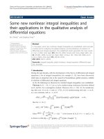
In order to represent certain sets in C" geometrically, it is convenient to
consider the image r(D) of Din absolute space {(r 1 , ... ,r.)E~":ri;:::O for
j = 1, ... , n}, under the map r: a--+ (la 1 l, ... , la.l). For example, B(O, r) and
P(O, (r 1 , r 2 )) in IC 2 have the representations shown in Figure 1.
If n > 2, we sometimes write z = (z', z.), where z' = (z 1 , ... , z._ 1 ) E IC"- 1 .
For example, if 0 < ri < 1, 1 :$; j :$; n, the domain
H(r) = {z E IC": z' E P'(O, r'), lz.l < 1} U {z E C", z' E P'(O, 1), r. < lz.l < 1}
can be represented schematically by Figure 2.
The pair (H(r), P(O, 1)) is called a (Euclidean) Hartogs figure; its significance
will become clear in Chapter II.
Notice that
for 1

:$;

j

:$;

n}


www.pdfgrip.com
4

I. Elementary Local Properties of Holomorphic Functions

•
T(z')

r'
T(H(r))

Figure 2. Representation of H(r) in absolute space.

is an n-dimensional real torus. So the representation in absolute space is
reasonable only for sets which are circled in the following sense.
Definition. A set Q c
T- 1(r(a))

=

en is circled (around 0) if for every a E Q the torus
{zEe:

Z

=

(alei 81 , ... , anei 8"),

0 S (}j S 2n}

lies in Q as well. A Reinhardt domain (centered at 0) is an open circled (around
0) set in e. A Reinhardt domain D is complete if for every a ED one has
P(O, r(a)) c D.
It is clear how to define the corresponding concepts for arbitrary centers.
B(O, r) and P(O, r) are complete Reinhardt domains, while the domain H(r)

in Figure 2 is a Reinhardt domain which is not complete.
Reinhardt domains appear naturally when one considers power series or
Laurent expansions of holomorphic functions (see §1.5 and Chapter II, §1).
Observe that a complete Reinhardt domain in C (centered at 0) is an open
disc with center 0; what are the Reinhardt domains in C?

1.2. The Cauchy-Riemann Equations
For D c !Rn, open, and kEN U {oo }, Ck(D) denotes the space of k times
continuously differentiable complex valued functions on D; we also write
C(D) instead of C 0 (D). We shall use the standard multi-index notation: if
!X = (rxl, ... ' rxn) E Nn and X =(xu ... ' Xn) E !Rn, one sets

Ia. I = rxl + ... + rxn, a! = rxl! .... an!,
x~

= x!'· ...

·x~",

rx

~

0(>0)

ifrxj

~

0(>0)

for 1 sj s n,


www.pdfgrip.com
5

§1. Holomorphic Functions

(1.5)
For f

E

Ck(D), k < oo, we define the Ck norm off over D by
lflk,D =

(1.6)

L

sup ID"l'(x)l;

aeN"xeD
jaj,;k

we write If I» instead of lflo,D• and if Dis clear from the context, we may write
lflk instead of lflk.D· The space Bk(D) = {! E Ck(D): lflk < oo} is complete in
the Ck norm l·lk, and hence Bk(D) is a Banach space. Similarly, the space
Ck(f5): = {! E Ck(D): D'r extends continuously to i5 for all ocE 1\J" with loci :$; k},
with the norm l·lk.D• is also a Banach space.
Turning to C" = IR 2 " with coordinates zi = xi + j=l Yi• one introduces
the partial differential operators
(1.7)

a~j = ~(a~j + ~ a:J.

The following rules are easily verified:

The multi-index notation (1.5) is extended to the operators (1.7) as follows: for
oc, {3 E 1\J",
(1.8)
We write Da for Dao and Dli for D07i; this should cause no confusion with (1.5).
Notice that f E Ck(D) if and only if Dalif E C(D) for all oc, f3 with loci + 1/31 :$; k.
We now introduce the class of functions which is the principal object of
study in this book.
Definition. Let D c C" be open. A function f: D-+ Cis called holomorphic

(on D) iff E C 1 (D) and f satisfies the system of partial differential equations
(1.9)

a! (z) = 0

ozj

for 1 :$;j :$;nand zED.

The space of holomorphic functions on D is denoted by (!}(D). More generally, if n is an arbitrary subset of C", we denote by (!}(Q) the collection of those
functions which are defined and holomorphic on some open neighborhood of
n, with the understanding that two such functions define the same element
in (!)(Q) if they agree on a neighborhood of Q. 1 A function f is said to be
hoJomorphic at the point a E C" iff E (!}( {a}).
The following result is an immediate consequence of the definitions and
standard calculus.
1 This identification can be formalized by introducing the language of germs of functions (see
Chapter VI, §4).


www.pdfgrip.com

6

I. Elementary Local Properties of Holomorphic Functions

Theorem 1.1. For any subset 0 of C", @(Q) is closed under pointwise addition
and multiplication. Any polynomial in z 1 , ... , z" with complex coefficients
is holomorphic on IC", and hence, by restriction, is in @(0). Iff, g E @(Q) and
g(z) # 0 for all zEO, thenfjgE@(Q).

Equation (1.9) is called the system of (homogeneous) Cauchy-Riemann
equations. Notice that any function f which satisfies (1.9) satisfies the CauchyRiemann equations in the zrcoordinate for any j, and hence is holomorphic
in each variable separately. It is a remarkable phenomenon of complex analysis
-discovered by F. Hartogs in 1906 [Har 2]-that conversely, any function
f: D -..IC which is holomorphic in each variable separately is holomorphic,
as defined above. This shows that the requirement that f E C 1 (D) can be
dropped in the definition of holomorphic function. The main difficulty in
Hartogs' Theorem is to show that a function f which satisfies (1.9) is locally
bounded. Assuming that f is bounded, it is quite elementary to show that (1.9)
implies f E C 00 (D) (see Exercise E.l.3 and Corollary 1.5 below).
In order to appreciate the strength of Hartogs' Theorem, the reader
should notice that the function f: IR 2 -.. IR defined by f(O) = 0 and f(x, y) =
xyj(x 4 + y 4 ) for (x, y) # 0 is coo (even real analytic) in each variable separately,
but is not bounded at 0.
The inhomogeneous system of Cauchy-Riemann equations
(1.10)

1 ~j

~

n,

where u 1 , ... , u" are given C 1 functions on D, will also be very important for
the study ofholomorphic functions. For n = 1, the system (1.10) is determined
(i.e., one equation for one unknown function, or two real equations for the
two real functions Ref, Imf), while for n > 1 (1.10) is overdetermined (more
equations than unknowns). This fact makes life in several variables harder,
and it accounts for many of the differences between the cases n = 1 and n > 1.
Notice that if there is a solution f E C 2 (D) of(l.lO), then the functions u 1 , •.• , u"

must satisfy the necessary integrability conditions
(1.11)

1 ~j, k

~

n;

(1.11) always holds in case n = 1, while it is quite restrictive in case n > 1.
We now give another interpretation for the solutions of the homogeneous
Cauchy-Riemann equations. Let f E C 1 (D); its differential dfa at a ED is the
unique IR-linear map IR 2 "-.. IR 2 which approximates f near a in the sense
that f(z) = f(a) + dfa(z- a)+ o(lz- al). 1 In terms of the real coordinates
(x 1 , y 1 , ..• , Xn, Yn) ofiC", one has
(1.12)
1 We use a standard notation from analysis: if A = A(x) is an expression which depends on x e ~·.
the statements A= O(lxl), and A= o(lxl) mean, respectively, that IA(x)l :S Clxl as lxl-+ 0 for
some constant C, and limlxl~o IA(x)l/lxl = 0.


www.pdfgrip.com
7

§1. Holomorphic Functions

where dxj, dyj are the differentials of the coordinate functions, i.e.,
Via the identification IR 2 " = IC" and IR 2 = IC, the differential dfa can be
viewed as a map IC" -+ IC which is IR-linear, though not necessarily IC-linear.
In particular, the differentials dxj and dyj are not linear over IC; for example,

if ( = (1, 0, ... , 0) E IR 2", then i( = (0, 1, 0, ... , 0), so that dx 1 (i() = 0, while
idx 1(( d = i. In complex analysis one therefore considers the differentials
dzj = dxj + idyj (this is IC-linear) and ~ = dxj- idyj (this is conjugate IClinear1) of the complex coordinate functions zj, 1 :s; j :s; n. A simple computation shows that
(1.13)
The first sum in (1.13) is denoted by ofa, or of(a), the second sum by fJfa, or
fJf(a). So one can say that
(1.14)

fEC 1 (D) is holomorphic<=>fJf

= O<=>df =of.

Theorem 1.2. AfunctionfEC 1 (D) satisfies the Cauchy-Riemann equations at

the point a ED if and only if its differential dfa at a is IC-linear. In particular,
f E @(D) if and only if df is IC-linear at every point.

PROOF. Since ofa is obviously IC-linear for any a ED, one implication is
trivial. For the other implication, suppose {Jk = ofjozk(a) =1- 0 for some k. Let
ak = ofjozk(a), and W = (0, ... , 1, 0, ... , 0) E IC", with the 1 in the kth place.
Then dfa(w) = ak + {Jk> and dfa(iw) = aki- {Jki = i(ak - {Jk) =1- idfa(w), so that
dfa is not linear over IC. •

We shall discuss these matters more systematically and in coordinate-free
form in Chapter III, §2.2; for the present, let us mention though that it is
Equation (1.13) for the differential of a C 1 function which motivates the
definition of the operators ojozj and a;a~ in (1.7).

1.3. The Cauchy Integral Formula on Polydiscs
As in the case of one complex variable, the basic local properties of holomorphic functions follow from an integral representation formula, which is

most easily established on polydiscs. Later we will consider an analogous
formula on the ball and on more general domains (see Chapter IV, §3.2 and
Chapter VII, §1).
1 A map 1: V---> W between two complex vector spaces V and W is conjugate ~:>linear if I is linear
over IR and if l(.!cv) = Il(v) for all .!c E C, v E V.


www.pdfgrip.com
8

I. Elementary Local Properties of Holomorphic Functions

Theorem 1.3. Let P = P(a, r) be a polydisc in IC" with multiradius r = (r 1 ,

•.. , rn).
Suppose f E C(P), and f is holomorphic in each variable separately, i.e.,Jor each
z E fi and 1 ::::;; j ::::;; n, the function fzJA.) = f(z 1 , ••• , zi-l, A., zi+l, ... , zn) is holomorphic on {A.EIC: lA.- ail< ri}. Then

(1.15)

f(z)=(2ni)-n

r

j(()d( 1 ••• d(n

Jv((l- Z1) ... ((n- Zn)

forzEP,

where boP= {'EIC": i(i- ail= ri, 1 ::;;j::::;; n}.

Notice that the region of integration b0 P in (1.15) is strictly smaller than the
topological boundary bP of P in case n > 1. b0 P is called the distinguished
boundary of P, and in many situations it plays the same role as the unit circle
in one complex variable (see Theorem 1.8 below for an example).
The integral in (1.15) is an example of an n-form integrated over the real
n-dimensional manifold b0 P (see Chapter III, §1). In terms of the standard
parametrization
(i

= ai + riei8J,

of b0 P(a, r), one has
(1.16)

(

J

g(() d( 1 ... d(n = i"r 1 ... rn (

J

g(((O))ei8 '

•••

ei 8"d0 1 ••• dOn

[0, 21t]"

b 0 P(a,r)

for any g E C(b0 P). For the time being, the reader may simply view the left side
in (1.16) as a shorthand notation for the right side.
PROOF. We use induction over the number of variables n. For n = 1 one has
the classical Cauchy integral formula, which we assume as known. Suppose
n > 1, and that the theorem has been proved for n- 1 variables. For zEP
fixed, apply the inductive hypothesis with respect to (z 2 , ••• , zn), obtaining

where a'
gives

= (a 2 , ••• , an),

r'

= (r 2 , ••• , rn). For ( 2 , ..• , (n fixed, the case

n

=1

(1.18)
Now substitute (1.18) into (1.17) and transform the iterated integral over
{1(1 - a 1 1 = rt} x b0 P'(a', r') into an integral over b0 P-use the parametrization (1.16). •

Remark 1.4. The continuity off was used only at the end ofthe proof. Weaker
conditions on f, for example f bounded and measurable, would work just as

well by basic results in integration theory. On the other hand, it is important


www.pdfgrip.com
9

§1. Holornorphic Functions

for the applications given below that (1.15) is an integral over b0 P, and not
just an iterated integral.

Corollary 1.5. Suppose f E C(D) (or just bounded on D) is holomorphic in each
variable separately. Then! E C00 (D) and, in particular,/ E l!/(D). For any IX E f\Jn,
D"f E l!/(D).
PROOF. Apply Theorem 1.3 to a polydisc P(a, r) cc D; in (1.15) it is legitimate
to differentiate under the integral sign as often as needed. •

Theorem 1.6 (Cauchy estimates). Let f

r)). Then,for all IX E f\Jn,

IX!

(1.19)
(1.20)

E l!I(P(a,

ID"f(a)l ::;; r" 1/IP(a,r);
ID"f(a)l ::;;

1X!(1X 1 + 2) ... (1Xn
(2ntra+2

+ 2)

II f

IIL'(P(a,r))·

Note that r" = ri' ... r:n, and for mE Z, IX+ m = (1X 1 + m, ... , 1Xn + m); for
1 ::;; p ::;; oo, U(D) denvtes the space of functions on D with 1/IP Lebesgue
integrable over D (with respect to Lebesgue measure on IR 2 n), and 11/IILP(Dl =
D lfiP)lfp.


PROOF. Fix 0 < p < r. Apply Theorem 1.3 to P(a, p) cc P(a, r) and differentiate under the integral sign, obtaining

(1.21)

D"f(a) = ~
(2nit

l
/(0 d( dCn
J P(a,p) (( - a)"+
1 .•.

1

b0

(see (1.5) for the multi-index notation used). After an obvious estimation of
(1.21) and taking the limit p--+ r, (1.19) follows. For (1.20), use (1.16) in (1.21),
multiply by p"+ 1 and estimate, obtaining

(1.22)

ID"f(a)lp"+ 1 ::;; (21X!)n
1t

l

1/(((0))Ipl ... Pn d01 ... dOn.

J[0,21t]n

The desired inequality follows after integrating (1.22) over 0 ::;; Pi ::;; ri,
1 ::;; j ::;; n, and transforming the n-fold integral in polar coordinates into a
volume integral. •
The estimate (1.20) is often used in the following form.

Corollary 1.7. For each IXE f\Jn, 1 ::;; p::;; oo, and
C = C{IX, p, n, D) such that
(1.23)

Q cc

D there is a constant

ID"/In::;; CII/IILP(Dl for all fel!I(D)nU(D).

The space l!/(D) n U(D) of holomorphic U functions on D will be denoted
by l!IU(D).