Chương 2 2 Phương Trình TUYẾN TÍNH

Confirming Pages

Chapter Two
Linear Programming:
Basic Concepts
Learning Objectives
After completing this chapter, you should be able to
1. Explain what linear programming is.
2. Identify the three key questions to be addressed in formulating any spreadsheet
model.
3. Name and identify the purpose of the four kinds of cells used in linear programming
spreadsheet models.
4. Formulate a basic linear programming model in a spreadsheet from a description of
the problem.
5. Present the algebraic form of a linear programming model from its formulation on a
spreadsheet.
6. Apply the graphical method to solve a two-variable linear programming problem.
7. Use Excel to solve a linear programming spreadsheet model.

The management of any organization regularly must make decisions about how to allocate its
resources to various activities to best meet organizational objectives. Linear programming is
a powerful problem-solving tool that aids management in making such decisions. It is applicable to both profit-making and not-for-profit organizations, as well as governmental agencies. The resources being allocated to activities can be, for example, money, different kinds
of personnel, and different kinds of machinery and equipment. In many cases, a wide variety
of resources must be allocated simultaneously. The activities needing these resources might
be various production activities (e.g., producing different products), marketing activities
(e.g., advertising in different media), financial activities (e.g., making capital investments),
or some other activities. Some problems might even involve activities of all these types (and
perhaps others), because they are competing for the same resources.
You will see as we progress that even this description of the scope of linear programming is not sufficiently broad. Some of its applications go beyond the allocation of resources.
However, activities always are involved. Thus, a recurring theme in linear programming is
the need to find the best mix of activities—which ones to pursue and at what levels.

Like the other management science techniques, linear programming uses a mathematical
model to represent the problem being studied. The word linear in the name refers to the form
of the mathematical expressions in this model. Programming does not refer to computer programming; rather, it is essentially a synonym for planning. Thus, linear programming means
the planning of activities represented by a linear mathematical model.
Because it comprises a major part of management science, linear programming takes up
several chapters of this book. Furthermore, many of the lessons learned about how to apply
linear programming also will carry over to the application of other management science
techniques.
This chapter focuses on the basic concepts of linear programming.
22

hil24064_ch02_022-063.indd 22

02/11/12 5:23 PM


Confirming Pages

2.1

2.1

A Case Study: The Wyndor Glass Co. Product-Mix Problem 23

A CASE STUDY: THE WYNDOR GLASS CO. PRODUCT-MIX PROBLEM
Jim Baker has had an excellent track record during his seven years as manager of new product
development for the Wyndor Glass Company. Although the company is a small one, it has
been experiencing considerable growth largely because of the innovative new products developed by Jim’s group. Wyndor’s president, John Hill, has often acknowledged publicly the key
role that Jim has played in the recent success of the company.
Therefore, John felt considerable confidence six months ago in asking Jim’s group to

develop the following new products:
• An 8-foot glass door with aluminum framing.
• A 4-foot 3 6-foot double-hung, wood-framed window.
Although several other companies already had products meeting these specifications, John
felt that Jim would be able to work his usual magic in introducing exciting new features that
would establish new industry standards.

Background
The Wyndor Glass Co. produces high-quality glass products, including windows and glass
doors that feature handcrafting and the finest workmanship. Although the products are expensive, they fill a market niche by providing the highest quality available in the industry for the
most discriminating buyers. The company has three plants that simultaneously produce the
components of its products.
Plant 1 produces aluminum frames and hardware.
Plant 2 produces wood frames.
Plant 3 produces the glass and assembles the windows and doors.
Because of declining sales for certain products, top management has decided to revamp
the company’s product line. Unprofitable products are being discontinued, releasing production capacity to launch the two new products developed by Jim Baker’s group if management
approves their release.
The 8-foot glass door requires some of the production capacity in Plants 1 and 3, but not
Plant 2. The 4-foot 3 6-foot double-hung window needs only Plants 2 and 3.
Management now needs to address two issues:
1. Should the company go ahead with launching these two new products?
2. If so, what should be the product mix—the number of units of each produced per week—
for the two new products?

Management’s Discussion of the Issues
Having received Jim Baker’s memorandum describing the two new products, John Hill now has
called a meeting to discuss the current issues. In addition to John and Jim, the meeting includes
Bill Tasto, vice president for manufacturing, and Ann Lester, vice president for marketing.
Let’s eavesdrop on the meeting.

John Hill (president): Bill, we will want to rev up to start production of these products as
soon as we can. About how much production output do you think we can achieve?
Bill Tasto (vice president for manufacturing): We do have a little available production
capacity, because of the products we are discontinuing, but not a lot. We should be able to
achieve a production rate of a few units per week for each of these two products.
John: Is that all?
Bill: Yes. These are complicated products requiring careful crafting. And, as I said, we
don’t have much production capacity available.
John: Ann, will we be able to sell several of each per week?
Ann Lester (vice president for marketing): Easily.

hil24064_ch02_022-063.indd 23

02/11/12 5:23 PM


Confirming Pages

An Application Vignette
Swift & Company is a diversified protein-producing business based in Greeley, Colorado. With annual sales of over
$8 billion, beef and related products are by far the largest
portion of the company’s business.
To improve the company’s sales and manufacturing performance, upper management concluded that it needed
to achieve three major objectives. One was to enable the
company’s customer service representatives to talk to their
more than 8,000 customers with accurate information
about the availability of current and future inventory while
considering requested delivery dates and maximum product age upon delivery. A second was to produce an efficient
shift-level schedule for each plant over a 28-day horizon. A
third was to accurately determine whether a plant can ship

a requested order-line-item quantity on the requested date

The issue is to find the most
profitable mix of the two
new products.

and time given the availability of cattle and constraints on
the plant’s capacity.
To meet these three challenges, a management science
team developed an integrated system of 45 linear programming models based on three model formulations to dynamically schedule its beef-fabrication operations at five plants
in real time as it receives orders. The total audited benefits
realized in the first year of operation of this system were
$12.74 million, including $12 million due to optimizing the
product mix. Other benefits include a reduction in orders lost,
a reduction in price discounting, and better on-time delivery.
Source: A. Bixby, B. Downs, and M. Self, “A Scheduling and
Capable-to-Promise Application for Swift & Company, Interfaces 36,
no. 1 (January–February 2006), pp. 69–86. (A link to this article is
provided on our website, www.mhhe.com/hillier5e.)

John: Good. Now there’s one more issue to resolve. With this limited production capacity,
we need to decide how to split it between the two products. Do we want to produce the same
number of both products? Or mostly one of them? Or even just produce as much as we can
of one and postpone launching the other one for a little while?
Jim Baker (manager of new product development): It would be dangerous to hold one
of the products back and give our competition a chance to scoop us.
Ann: I agree. Furthermore, launching them together has some advantages from a marketing standpoint. Since they share a lot of the same special features, we can combine the
advertising for the two products. This is going to make a big splash.
John: OK. But which mixture of the two products is going to be most profitable for the
company?

Bill: I have a suggestion.
John: What’s that?
Bill: A couple times in the past, our Management Science Group has helped us with these
same kinds of product-mix decisions, and they’ve done a good job. They ferret out all the
relevant data and then dig into some detailed analysis of the issue. I’ve found their input
very helpful. And this is right down their alley.
John: Yes, you’re right. That’s a good idea. Let’s get our Management Science Group
working on this issue. Bill, will you coordinate with them?
The meeting ends.

The Management Science Group Begins Its Work
At the outset, the Management Science Group spends considerable time with Bill Tasto to
clarify the general problem and specific issues that management wants addressed. A particular concern is to ascertain the appropriate objective for the problem from management’s
viewpoint. Bill points out that John Hill posed the issue as determining which mixture of the
two products is going to be most profitable for the company.
Therefore, with Bill’s concurrence, the group defines the key issue to be addressed as
follows.
Question: Which combination of production rates (the number of units produced per week) for
the two new products would maximize the total profit from both of them?

The group also concludes that it should consider all possible combinations of production rates
of both new products permitted by the available production capacities in the three plants. For
example, one alternative (despite Jim Baker’s and Ann Lester’s objections) is to forgo producing one of the products for now (thereby setting its production rate equal to zero) in order
24

hil24064_ch02_022-063.indd 24

02/11/12 5:23 PM

Confirming Pages

2.2

TABLE 2.1

Formulating the Wyndor Problem on a Spreadsheet 25

Production Time Used
for Each Unit Produced

Data for the Wyndor
Glass Co. Product-Mix
Problem

Plant

Doors

Windows

Available per Week

1
2
3
Unit profit

1 hour
0

3 hours
$300

0
2 hours
2 hours
$500

4 hours
12 hours
18 hours

to produce as much as possible of the other product. (We must not neglect the possibility that
maximum profit from both products might be attained by producing none of one and as much
as possible of the other.)
The Management Science Group next identifies the information it needs to gather to conduct this study:
1. Available production capacity in each of the plants.
2. How much of the production capacity in each plant would be needed by each product.
3. Profitability of each product.
Concrete data are not available for any of these quantities, so estimates have to be made.
Estimating these quantities requires enlisting the help of key personnel in other units of the
company.
Bill Tasto’s staff develops the estimates that involve production capacities. Specifically,
the staff estimates that the production facilities in Plant 1 needed for the new kind of doors
will be available approximately four hours per week. (The rest of the time Plant 1 will continue with current products.) The production facilities in Plant 2 will be available for the new
kind of windows about 12 hours per week. The facilities needed for both products in Plant 3
will be available approximately 18 hours per week.
The amount of each plant’s production capacity actually used by each product depends
on its production rate. It is estimated that each door will require one hour of production time
in Plant 1 and three hours in Plant 3. For each window, about two hours will be needed in

Plant 2 and two hours in Plant 3.
By analyzing the cost data and the pricing decision, the Accounting Department estimates
the profit from the two products. The projection is that the profit per unit will be $300 for the
doors and $500 for the windows.
Table 2.1 summarizes the data now gathered.
The Management Science Group recognizes this as being a classic product-mix problem.
Therefore, the next step is to develop a mathematical model—that is, a linear programming
model—to represent the problem so that it can be solved mathematically. The next four sections
focus on how to develop this model and then how to solve it to find the most profitable mix
between the two products, assuming the estimates in Table 2.1 are accurate.

Review
Questions

2.2

1.
2.
3.
4.

What were the two issues addressed by management?
The Management Science Group was asked to help analyze which of these issues?
How did this group define the key issue to be addressed?
What information did the group need to gather to conduct its study?

FORMULATING THE WYNDOR PROBLEM ON A SPREADSHEET
Spreadsheets provide a powerful and intuitive tool for displaying and analyzing many management problems. We now will focus on how to do this for the Wyndor problem with the
popular spreadsheet package Microsoft Excel.1
1

Other spreadsheet packages with similar capabilities also are available, and the basic ideas presented here
are still applicable.

hil24064_ch02_022-063.indd 25

02/11/12 5:23 PM


Confirming Pages

26 Chapter Two

Linear Programming: Basic Concepts

Formulating a Spreadsheet Model for the Wyndor Problem
Excel Tip: Cell shading
and borders can be added
by using the borders button and the fill color button
in the Font Group of the
Home tab.

Excel Tip: See the margin
notes in Section 1.2 for tips
on adding range names.

These are the three key
questions to be addressed
in formulating any spreadsheet model.

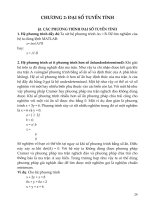
Figure 2.1 displays the Wyndor problem by transferring the data in Table 2.1 onto a spreadsheet. (Columns E and F are being reserved for later entries described below.) We will refer
to the cells showing the data as data cells. To distinguish the data cells from other cells in
the spreadsheet, they are shaded light blue. (In the textbook figures, the light blue shading
appears as light gray.) The spreadsheet is made easier to interpret by using range names. (As
mentioned in Section 1.2, a range name is simply a descriptive name given to a cell or
range of cells that immediately identifies what is there. Excel allows you to use range names
instead of the corresponding cell addresses in Excel equations, since this usually makes the
equations much easier to interpret at a glance.) The data cells in the Wyndor Glass Co. problem are given the range names UnitProfit (C4:D4), HoursUsedPerUnitProduced (C7:D9),
and Hours Available (G7:G9). To enter a range name, first select the range of cells, then
click in the name box on the left of the formula bar above the spreadsheet and type a name.
(See Appendix A for further details about defining and using range names.)
Three questions need to be answered to begin the process of using the spreadsheet to formulate a mathematical model (in this case, a linear programming model) for the problem.
1. What are the decisions to be made?
2. What are the constraints on these decisions?
3. What is the overall measure of performance for these decisions?
The preceding section described how Wyndor’s Management Science Group spent considerable time with Bill Tasto, vice president for manufacturing, to clarify management’s view of
their problem. These discussions provided the following answers to these questions.

Some students find it
helpful to organize their
thoughts by answering
these three key questions
before beginning to formulate the spreadsheet model.

The changing cells contain
the decisions to be made.

1. The decisions to be made are the production rates (number of units produced per week) for
the two new products.
2. The constraints on these decisions are that the number of hours of production time used

per week by the two products in the respective plants cannot exceed the number of hours
available.
3. The overall measure of performance for these decisions is the total profit per week from
the two products.
Figure 2.2 shows how these answers can be incorporated into the spreadsheet. Based on
the first answer, the production rates of the two products are placed in cells C12 and D12
to locate them in the columns for these products just under the data cells. Since we don’t
know yet what these production rates should be, they are just entered as zeroes in Figure 2.2.
(Actually, any trial solution can be entered, although negative production rates should be
excluded since they are impossible.) Later, these numbers will be changed while seeking the
best mix of production rates. Therefore, these cells containing the decisions to be made are
called changing cells. To highlight the changing cells, they are shaded bright yellow with a
light border. (In the textbook figures, the bright yellow appears as gray.) The changing cells
are given the range name UnitsProduced (C12:D12).

FIGURE 2.1
The initial spreadsheet for
the Wyndor problem after
transferring the data in
Table 2.1 into data cells.

A
1

B

C

D

F

G

Wyndor Glass Co. Product-Mix Problem

2
3
4

Unit Profit

Doors

Windows

$300

$500

5

Hours

6

hil24064_ch02_022-063.indd 26

E

Hours Used per Unit Produced

Available

7

Plant 1

1

0

4

8

Plant 2

0

2

12

9

Plant 3

3

2

18

02/11/12 5:23 PM


Confirming Pages

2.2

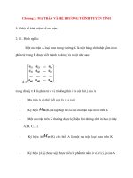
FIGURE 2.2
The complete spreadsheet
for the wyndor problem
with an initial trial solution (both production rates
equal to zero) entered into
the changing cells (C12
and D12).

A
1

B

C

Formulating the Wyndor Problem on a Spreadsheet 27

D

E

F

G

Wyndor Glass Co. Product-Mix Problem

2
3
4

Unit Profit

Doors

Windows

$300

$500

5
6

Hours Used per Unit Produced

Hours

Hours

Used

Available

7

Plant 1

1

0

0

≤

4

8

Plant 2

0

2

0

≤

12

9

Plant 3

3

2

0

≤

18

Doors

Windows

Total Profit

0

0

$0

10

11
12

The colon in C7:D9 is
Excel shorthand for the
range from C7 to D9; that
is, the entire block of cells
in column C or D and in
row 7, 8, or 9.

Units Produced

Using the second answer, the total number of hours of production time used per week by
the two products in the respective plants is entered in cells E7, E8, and E9, just to the right of
the corresponding data cells. The total number of production hours depends on the production
rates of the two products, so this total is zero when the production rates are zero. With positive production rates, the total number of production hours used per week in a plant is the sum
of the production hours used per week by the respective products. The production hours used
by a product is the number of hours needed for each unit of the product times the number of
units being produced. Therefore, when positive numbers are entered in cells C12 and D12 for
the number of doors and windows to produce per week, the data in cells C7:D9 are used to
calculate the total production hours per week as follows:
Production hours in Plant 1 5 1(# of doors) 1 0(# of windows)
Production hours in Plant 2 5 0(# of doors) 1 2(# of windows)
Production hours in Plant 3 5 3(# of doors) 1 2(# of windows)
Consequently, the Excel equations for the three cells in column E are
E7 5 C7*C12 1 D7*D12
E8 5 C8*C12 1 D8*D12
E9 5 C9*C12 1 D9*D12

Output cells show quantities that are calculated from

the changing cells.

The SUMPRODUCT function is used extensively in
linear programming spreadsheet models.

hil24064_ch02_022-063.indd 27

where each asterisk denotes multiplication. Since each of these cells provides output that
depends on the changing cells (C12 and D12), they are called output cells.
Notice that each of the equations for the output cells involves the sum of two products.
There is a function in Excel called SUMPRODUCT that will sum up the product of each
of the individual terms in two different ranges of cells when the two ranges have the same
number of rows and the same number of columns. Each product being summed is the product of a term in the first range and the term in the corresponding location in the second
range. For example, consider the two ranges, C7:D7 and C12:D12, so that each range has
one row and two columns. In this case, SUMPRODUCT (C7:D7, C12:D12) takes each of
the individual terms in the range C7:D7, multiplies them by the corresponding term in the
range C12:D12, and then sums up these individual products, just as shown in the first equation above. Applying the range name for UnitsProduced (C12:D12), the formula becomes
SUMPRODUCT(C7:D7, UnitsProduced). Although optional with such short equations, this
function is especially handy as a shortcut for entering longer equations.
The formulas in the output cells E7:E9 are very similar. Rather than typing each of these
formulas separately into the three cells, it is quicker (and less prone to typos) to type the
formula just once in E7 and then copy the formula down into cells E8 and E9. To do this,
first enter the formula 5SUMPRODUCT(C7:D7, UnitsProduced) in cell E7. Then select cell

02/11/12 5:23 PM


Confirming Pages

28 Chapter Two

Linear Programming: Basic Concepts

You can make the column
absolute and the row relative (or vice versa) by putting a $ sign in front of only
the letter (or number) of the
cell reference.
Excel Tip: After entering
a cell reference, repeatedly
pressing the F4 key (or
command-T on a Mac) will
rotate among the four possibilities of relative and absolute references (e.g., C12,
$C$12, C$12, $C12).

E7 and drag the fill handle (the small box on the lower right corner of the cell cursor) down
through cells E8 and E9.
When copying formulas, it is important to understand the difference between relative and
absolute references. In the formula in cell E7, the reference to cells C7:D7 is based upon the
relative position to the cell containing the formula. In this case, this means the two cells in the
same row and immediately to the left. This is known as a relative reference. When this formula is copied to new cells using the fill handle, the reference is automatically adjusted to refer
to the new cell(s) at the same relative location (the two cells in the same row and immediately
to the left). The formula in E8 becomes  5SUMPRODUCT(C8:D8, UnitsProduced) and the
formula in E9 becomes  5SUMPRODUCT(C9:D9, UnitsProduced). This is exactly what we
want, since we always want the hours used at a given plant to be based upon the hours used per
unit produced at that same plant (the two cells in the same row and immediately to the left).
In contrast, the reference to the UnitsProduced in E7 is called an absolute reference.
These references do not change when they are filled into other cells but instead always refer
to the same absolute cell locations.
To make a relative reference, simply enter the cell address (e.g., C7:D7). References
referred to by a range name are treated as absolute references. Another way to make an absolute reference to a range of cells is to put $ signs in front of the letter and number of the cell

reference (e.g., $C$12:$D$12). See Appendix A for more details about relative and absolute
referencing and copying formulas.
Next, # signs are entered in cells F7, F8, and F9 to indicate that each total value to their
left cannot be allowed to exceed the corresponding number in column G. (On the computer #
(or $) is often represented as ,5 (or .5), since there is no # (or $) key on the keyboard.)
The spreadsheet still will allow you to enter trial solutions that violate the # signs. However,
these # signs serve as a reminder that such trial solutions need to be rejected if no changes are
made in the numbers in column G.
Finally, since the answer to the third question is that the overall measure of performance is
the total profit from the two products, this profit (per week) is entered in cell G12. Much like
the numbers in column E, it is the sum of products. Since cells C4 and D4 give the profit from
each door and window produced, the total profit per week from these products is
Profit 5 $300(# of doors) 1 $500(# of windows)

One easy way to enter a
# (or $) in a spreadsheet
is to type , (or .) with
underlining turned on.

Hence, the equation for cell G12 is
G12 5 SUMPRODUCT(C4:D4, C12:D12)
Utilizing range names of TotalProfit (G12), UnitProfit (C4:D4), and UnitsProduced
(C12:D12), this equation becomes
TotalProfit 5 SUMPRODUCT(UnitProfit, UnitsProduced)

The objective cell contains
the overall measure of performance for the decisions
in the changing cells.

hil24064_ch02_022-063.indd 28

This is a good example of the benefit of using range names for making the resulting equation
easier to interpret.
TotalProfit (G12) is a special kind of output cell. It is our objective to make this cell as
large as possible when making decisions regarding production rates. Therefore, TotalProfit
(G12) is referred to as the objective cell. This cell is shaded orange with a heavy border.
(In the textbook figures, the orange appears as gray and is distinguished from the changing
cells by its darker shading and heavy border.)
The bottom of Figure 2.3 summarizes all the formulas that need to be entered in the Hours
Used column and in the Total Profit cell. Also shown is a summary of the range names
(in alphabetical order) and the corresponding cell addresses.
This completes the formulation of the spreadsheet model for the Wyndor problem.
With this formulation, it becomes easy to analyze any trial solution for the production
rates. Each time production rates are entered in cells C12 and D12, Excel immediately calculates the output cells for hours used and total profit. For example, Figure  2.4 shows the
spreadsheet when the production rates are set at four doors per week and three windows
per week. Cell G12 shows that this yields a total profit of $2,700 per week. Also note that
E7  5 G7, E8 , G8, and E9  5 G9, so the # signs in column F are all satisfied. Thus, this

02/11/12 5:23 PM


Confirming Pages

2.2

FIGURE 2.3
The spreadsheet model
for the Wyndor problem,
including the formulas for
the objective cell TotalProfit (G12) and the other

output cells in column E,
where the goal is to maximize the objective cell.

A
1

B

C

Formulating the Wyndor Problem on a Spreadsheet 29

D

E

F

G

Wyndor Glass Co. Product-Mix Problem

2
3
Unit Profit

4

Doors

Windows

$300

$500

5
6

Hours Used per Unit Produced

Hours

Hours

Used

Available

7

Plant 1

1

0

0

≤

4

8

Plant 2

0

2

0

≤

12

9

Plant 3

3

2

0

≤

18

Doors

Windows

Total Profit

0

0

$0

10
11
12

Units Produced

Range Name

E

Cell

HoursAvailable
G7:G9
HoursUsed
E7:E9
HoursUsedPerUnitProduced C7:D9

TotalProfit
G12
UnitProfit
C4:D4
UnitsProduced
C12:D12

5

Hours

6
7
8
9

Used
=SUMPRODUCT(C7:D7, UnitsProduced)
=SUMPRODUCT(C8:D8, UnitsProduced)
=SUMPRODUCT(C9:D9, UnitsProduced)
G

FIGURE 2.4
The spreadsheet for the
Wyndor problem with
a new trial solution
entered into the changing cells, UnitsProduced
(C12:D12).

A

1

B

C

11

Total Profit

12

=SUMPRODUCT(UnitProfit, UnitsProduced)

D

E

F

G

Wyndor Glass Co. Product-Mix Problem

2
3
4

Unit Profit

Doors

Windows

$300

$500

5
6

Hours Used per Unit Produced

Hours

Hours

Used

Available

7

Plant 1

1

0

8

Plant 2

0

9

Plant 3

3
Doors

Windows

Total Profit

4

3

$2,700

4

≤

4

2

6

≤

12

2

18

≤

18

10
11
12

Units Produced

trial solution is feasible. However, it would not be feasible to further increase both production
rates, since this would cause E7 . G7 and E9 . G9.
Does this trial solution provide the best mix of production rates? Not necessarily. It might
be possible to further increase the total profit by simultaneously increasing one production
rate and decreasing the other. However, it is not necessary to continue using trial and error to
explore such possibilities. We shall describe in Section 2.5 how the Excel Solver can be used
to quickly find the best (optimal) solution.

This Spreadsheet Model Is a Linear Programming Model
The spreadsheet model displayed in Figure 2.3 is an example of a linear programming model.

The reason is that it possesses all the following characteristics.

hil24064_ch02_022-063.indd 29

02/11/12 5:23 PM


Confirming Pages

30 Chapter Two

Linear Programming: Basic Concepts

Characteristics of a Linear Programming Model on a Spreadsheet
1. Decisions need to be made on the levels of a number of activities, so changing cells are
used to display these levels. (The two activities for the Wyndor problem are the production
of the two new products, so the changing cells display the number of units produced per
week for each of these products.)
2. These activity levels can have any value (including fractional values) that satisfy a number
of constraints. (The production rates for Wyndor’s new products are restricted only by the
constraints on the number of hours of production time available in the three plants.)
3. Each constraint describes a restriction on the feasible values for the levels of the activities, where a constraint commonly is displayed by having an output cell on the left, a
mathematical sign (#, $, or 5) in the middle, and a data cell on the right. (Wyndor’s three
constraints involving hours available in the plants are displayed in Figures 2.2–2.4 by having output cells in column E, # signs in column F, and data cells in column G.)
4. The decisions on activity levels are to be based on an overall measure of performance,
which is entered in the objective cell. The goal is to either maximize the objective cell
or minimize the objective cell, depending on the nature of the measure of performance.
(Wyndor’s overall measure of performance is the total profit per week from the two new
products, so this measure has been entered in the objective cell G12, where the goal is to
maximize this objective cell.)

5. The Excel equation for each output cell (including the objective cell) can be expressed as
a SUMPRODUCT function,2 where each term in the sum is the product of a data cell and
a changing cell. (The bottom of Figure 2.3 shows how a SUMPRODUCT function is used
for each output cell for the Wyndor problem.)
Linear programming models are not the only models that can have characteristics 1, 3, and 4.
However, characteristics 2 and 5 are key assumptions of linear programming. Therefore, these
are the two key characteristics that together differentiate a linear programming model from
other kinds of mathematical models that can be formulated on a spreadsheet.
Characteristic 2 rules out situations where the activity levels need to have integer values.
For example, such a situation would arise in the Wyndor problem if the decisions to be made
were the total numbers of doors and windows to produce (which must be integers) rather
than the numbers per week (which can have fractional values since a door or window can be
started in one week and completed in the next week). When the activity levels do need to have
integer values, a similar kind of model (called an integer programming model) is used instead
by making a small adjustment on the spreadsheet, as will be illustrated in Section 3.2.
Characteristic 5 describes the so-called proportionality assumption of linear programming,
which states that each term in an output cell must be proportional to a particular changing cell.
This prohibits those cases where the Excel equation for an output cell cannot be expressed
as a SUMPRODUCT function. To illustrate such a case, suppose that the weekly profit from
producing Wyndor’s new windows can be more than doubled by doubling the production rate
because of economies in marketing larger amounts. This would mean that this weekly profit
is not simply proportional to this production rate, so the Excel equation for the objective cell
would need to be more complicated than a SUMPRODUCT function. Consideration of how
to formulate such models will be deferred to Chapter 8.

Summary of the Formulation Procedure
The procedure used to formulate a linear programming model on a spreadsheet for the Wyndor
problem can be adapted to many other problems as well. Here is a summary of the steps involved
in the procedure.
1. Gather the data for the problem (such as summarized in Table 2.1 for the Wyndor problem).

2. Enter the data into data cells on a spreadsheet.
3. Identify the decisions to be made on the levels of activities and designate changing cells
for displaying these decisions.
2
There also are some special situations where a SUM function can be used instead because all the numbers
that would have gone into the corresponding data cells are 1’s.

hil24064_ch02_022-063.indd 30

02/11/12 5:23 PM


Confirming Pages

2.3

The Mathematical Model in the Spreadsheet 31

4. Identify the constraints on these decisions and introduce output cells as needed to specify
these constraints.
5. Choose the overall measure of performance to be entered into the objective cell.
6. Use a SUMPRODUCT function to enter the appropriate value into each output cell (including the objective cell).
This procedure does not spell out the details of how to set up the spreadsheet. There generally are alternative ways of doing this rather than a single “right” way. One of the great
strengths of spreadsheets is their flexibility for dealing with a wide variety of problems.

Review
Questions

2.3

1. What are the three questions that need to be answered to begin the process of formulating a
linear programming model on a spreadsheet?
2. What are the roles for the data cells, the changing cells, the output cells, and the objective cell
when formulating such a model?
3. What is the form of the Excel equation for each output cell (including the objective cell) when
formulating such a model?

THE MATHEMATICAL MODEL IN THE SPREADSHEET

A linear programming
model can be formulated
either as a spreadsheet
model or as an algebraic
model.

There are two widely used methods for formulating a linear programming model. One is to
formulate it directly on a spreadsheet, as described in the preceding section. The other is to
use algebra to present the model. The two versions of the model are equivalent. The only difference is whether the language of spreadsheets or the language of algebra is used to describe
the model. Both versions have their advantages, and it can be helpful to be bilingual. For
example, the two versions lead to different, but complementary, ways of analyzing problems
like the Wyndor problem (as discussed in the next two sections). Since this book emphasizes
the spreadsheet approach, we will only briefly describe the algebraic approach.

Formulating the Wyndor Model Algebraically
The reasoning for the algebraic approach is similar to that for the spreadsheet approach. In
fact, except for making entries on a spreadsheet, the initial steps are just as described in the
preceding section for the Wyndor problem.
1. Gather the relevant data (Table 2.1 in Section 2.1).
2. Identify the decisions to be made (the production rates for the two new products).
3. Identify the constraints on these decisions (the production time used in the respective

plants cannot exceed the amount available).
4. Identify the overall measure of performance for these decisions (the total profit from the
two products).
5. Convert the verbal description of the constraints and measure of performance into quantitative expressions in terms of the data and decisions (see below).
To start performing step 5, note that Table 2.1 indicates that the number of hours of production time available per week for the two new products in the respective plants are 4, 12,
and 18. Using the data in this table for the number of hours used per door or window produced
then leads to the following quantitative expressions for the constraints:
Plant 1:
Plant 2:
Plant 3:

# 4
2(# of windows) # 12
3(# of doors) 1 2(# of windows) # 18
(# of doors)

In addition, negative production rates are impossible, so two other constraints on the decisions are
(# of doors) $ 0

(# of windows) $ 0

The overall measure of performance has been identified as the total profit from the two
products. Since Table  2.1 gives the unit profits for doors and windows as $300 and $500,

hil24064_ch02_022-063.indd 31

02/11/12 5:23 PM


Confirming Pages

32 Chapter Two

Linear Programming: Basic Concepts

respectively, the expression obtained in the preceding section for the total profit per week
from these products is
Profit 5 $300(# of doors) 1 $500(# of windows)
The goal is to make the decisions (number of doors and number of windows) so as to maximize this profit, subject to satisfying all the constraints identified above.
To state this objective in a compact algebraic model, we introduce algebraic symbols to
represent the measure of performance and the decisions. Let
P  5 Profit (total profit per week from the two products, in dollars)
D  5 # of doors (number of the special new doors to be produced per week)
W 5 # of windows (number of the special new windows to be produced per week)
Substituting these symbols into the above expressions for the constraints and the measure of
performance (and dropping the dollar signs in the latter expression), the linear programming
model for the Wyndor problem now can be written in algebraic form as shown below.
Algebraic Model
Choose the values of D and W so as to maximize
P 5 300D 1 500W
subject to satisfying all the following constraints:
# 4
2W # 12
3D 1 2W # 18
D

and
D$0

W$0

Terminology for Linear Programming Models
Much of the terminology of algebraic models also is sometimes used with spreadsheet models. Here are the key terms for both kinds of models in the context of the Wyndor problem.
1. D and W (or C12 and D12 in Figure 2.3) are the decision variables.
2. 300D  1  500W [or SUMPRODUCT (UnitProfit, UnitsProduced)] is the objective
function.
3. P (or G12) is the value of the objective function (or objective value for short).
4. D $ 0 and W $ 0 (or C12 $ 0 and D12 $ 0) are called the nonnegativity constraints
(or nonnegativity conditions).
5. The other constraints are referred to as functional constraints (or structural constraints).
6. The parameters of the model are the constants in the algebraic model (the numbers in the
data cells).
7. Any choice of values for the decision variables (regardless of how desirable or undesirable
the choice) is called a solution for the model.
8. A feasible solution is one that satisfies all the constraints, whereas an infeasible
solution violates at least one constraint.
9. The best feasible solution, the one that maximizes P (or G12), is called the optimal
solution. (It is possible to have a tie for the best feasible solution, in which case all the
tied solutions are called optimal solutions.)

Comparisons
Management scientists
often use algebraic models,
but managers generally prefer spreadsheet models.

hil24064_ch02_022-063.indd 32

So what are the relative advantages of algebraic models and spreadsheet models? An algebraic model provides a very concise and explicit statement of the problem. Sophisticated
software packages that can solve huge problems generally are based on algebraic models
because of both their compactness and their ease of use in rescaling the size of a problem.

02/11/12 5:23 PM


Confirming Pages

2.4

The Graphical Method for Solving Two-Variable Problems 33

Management science practitioners with an extensive mathematical background find algebraic
models very useful. For others, however, spreadsheet models are far more intuitive. Both
managers and business students training to be managers generally live with spreadsheets, not
algebraic models. Therefore, the emphasis throughout this book is on spreadsheet models.

Review
Questions

2.4

1. When formulating a linear programming model, what are the initial steps that are the same
with either a spreadsheet formulation or an algebraic formulation?
2. When formulating a linear programming model algebraically, algebraic symbols need to be
introduced to represent which kinds of quantities in the model?
3. What are decision variables for a linear programming model? The objective function? Nonnegativity constraints? Functional constraints?
4. What is meant by a feasible solution for the model? An optimal solution?

THE GRAPHICAL METHOD FOR SOLVING TWO-VARIABLE PROBLEMS

graphical method

The graphical method provides helpful intuition about
linear programming.

Linear programming problems having only two decision variables, like the Wyndor problem,
can be solved by a graphical method.
Although this method cannot be used to solve problems with more than two decision variables (and most linear programming problems have far more than two), it still is well worth
learning. The procedure provides geometric intuition about linear programming and what it is
trying to achieve. This intuition is helpful in analyzing larger problems that cannot be solved
directly by the graphical method.
It is more convenient to apply the graphical method to the algebraic version of the linear programming model rather than the spreadsheet version. We shall briefly illustrate the
method by using the algebraic model obtained for the Wyndor problem in the preceding section. (A far more detailed description of the graphical method, including its application to the
Wyndor problem, is provided in the supplement to this chapter on the CD-ROM.) For this
purpose, keep in mind that
D 5 Production rate for the special new doors (the number in changing cell C12 of the
spreadsheet)
W 5 Production rate for the special new windows (the number in changing cell D12 of
the spreadsheet)
The key to the graphical method is the fact that possible solutions can be displayed as
points on a two-dimensional graph that has a horizontal axis giving the value of D and a vertical axis giving the value of W. Figure 2.5 shows some sample points.
Notation: Either (D, W) 5 (2, 3) or just (2, 3) refers to the solution where D 5 2 and W 5 3,
as well as to the corresponding point in the graph. Similarly, (D, W) 5 (4, 6) means D 5 4 and
W 5 6, whereas the origin (0, 0) means D 5 0 and W 5 0.

feasible region
The points in the feasible
region are those that satisfy
every constraint.

hil24064_ch02_022-063.indd 33

To find the optimal solution (the best feasible solution), we first need to display graphically where the feasible solutions are. To do this, we must consider each constraint, identify
the solutions graphically that are permitted by that constraint, and then combine this information to identify the solutions permitted by all the constraints. The solutions permitted by all
the constraints are the feasible solutions and the portion of the two-dimensional graph where
the feasible solutions lie is referred to as the feasible region.
The shaded region in Figure 2.6 shows the feasible region for the Wyndor problem. We
now will outline how this feasible region was identified by considering the five constraints
one at a time.
To begin, the constraint D $ 0 implies that consideration must be limited to points that lie
on or to the right of the W axis. Similarly, the constraint W $ 0 restricts consideration to the
points on or above the D axis.
Next, consider the first functional constraint, D # 4, which limits the usage of Plant 1 for
producing the special new doors to a maximum of four hours per week. The solutions permitted by this constraint are those that lie on, or to the left of, the vertical line that intercepts the
D axis at D 5 4, as indicated by the arrows pointing to the left from this line in Figure 2.6.

02/11/12 5:23 PM


Confirming Pages

34 Chapter Two

Linear Programming: Basic Concepts
W

FIGURE 2.5
Graph showing the points
(D, W) 5 (2, 3) and
(D, W) 5 (4, 6) for the
Wyndor Glass Co.
product-mix problem.

Production Rate (units per week) for Windows

8

–1

(4, 6)

6
5
4

A product mix of
D = 2 and W = 3
(2, 3)

3
2
1

–2

A product mix of
D = 4 and W = 6

7

Origin

0

1

–1

2
3
4
5
6
7
Production Rate (units per week) for Doors

8

D

–2

The second functional constraint, 2W # 12, has a similar effect, except now the boundary of its permissible region is given by a horizontal line with the equation, 2W  5  12
(or W 5 6), as indicated by the arrows pointing downward from this line in Figure 2.6. The
line forming the boundary of what is permitted by a constraint is sometimes referred to as
W

FIGURE 2.6

10

3D + 2W = 18

Production Rate for Windows

Graph showing how the
feasible region is formed
by the constraint boundary lines, where the
arrows indicate which
side of each line is permitted by the corresponding
constraint.

8
D=4
2W = 12

6

4
Feasible
region
2

0

hil24064_ch02_022-063.indd 34

2

4
6
Production Rate for Doors

8

D

02/11/12 5:23 PM


Confirming Pages

2.4

For any constraint with an
inequality sign, its constraint boundary equation
is obtained by replacing the
inequality sign by an equality sign.

The Graphical Method for Solving Two-Variable Problems 35

a constraint boundary line, and its equation may be called a constraint boundary
equation. Frequently, a constraint boundary line is identified by its equation.
For each of the first two functional constraints, D # 4 and 2W # 12, note that the equation
for the constraint boundary line (D 5 4 and 2W 5 12, respectively) is obtained by replacing
the inequality sign with an equality sign. For any constraint with an inequality sign (whether
a functional constraint or a nonnegativity constraint), the general rule for obtaining its constraint boundary equation is to substitute an equality sign for the inequality sign.
We now need to consider one more functional constraint, 3D  1 2W # 18. Its constraint
boundary equation
3D 1 2W 5 18
includes both variables, so the boundary line it represents is neither a vertical line nor a horizontal line. Therefore, the boundary line must intercept (cross through) both axes somewhere.
But where?
When a constraint boundary line is neither a vertical line nor a horizontal line, the line intercepts

the D axis at the point on the line where W 5 0. Similarly, the line intercepts the W axis at the
point on the line where D 5 0.

Hence, the constraint boundary line 3D 1 2W 5 18 intercepts the D axis at the point where
W 5 0.
When W 5 0, 3D 1 2W 5 18
becomes 3D 5 18
so the intercept with the D axis is at
D5 6
The location of a slanting
constraint boundary line is
found by identifying where
it intercepts each of the two
axes.

Checking whether (0, 0)
satisfies a constraint indicates which side of the
constraint boundary line
satisfies the constraint.

Similarly, the line intercepts the W axis where D 5 0.
When D 5 0, 3D 1 2W 5 18
becomes 2W 5 18
so the intercept with the D axis is at
W5 9
Consequently, the constraint boundary line is the line that passes through these two intercept
points, as shown in Figure 2.6.
As indicated by the arrows emanating from this line in Figure 2.6, the solutions permitted
by the constraint 3D  1 2W # 18 are those that lie on the origin side of the constraint boundary line 3D  1 2W  5 18. The easiest way to verify this is to check whether the origin itself,
(D, W) 5 (0, 0), satisfies the constraint.3 If it does, then the permissible region lies on the side of

the constraint boundary line where the origin is. Otherwise, it lies on the other side. In this case,
3(0) 1 2(0) 5 0
so (D, W) 5 (0, 0) satisfies
3D 1 2W # 18
(In fact, the origin satisfies any constraint with a # sign and a positive right-hand side.)
A feasible solution for a linear programming problem must satisfy all the constraints
simultaneously. The arrows in Figure 2.6 indicate that the nonnegative solutions permitted by
each of these constraints lie on the side of the constraint boundary line where the origin is (or
on the line itself). Therefore, the feasible solutions are those that lie nearer to the origin than
all three constraint boundary lines (or on the line nearest the origin).
Having identified the feasible region, the final step is to find which of these feasible solutions is the best one—the optimal solution. For the Wyndor problem, the objective happens to
be to maximize the total profit per week from the two products (denoted by P). Therefore, we
want to find the feasible solution (D, W) that makes the value of the objective function
P 5 300D 1 500W
as large as possible.
To accomplish this, we need to be able to locate all the points (D, W) on the graph that give
a specified value of the objective function. For example, consider a value of P 5 1,500 for the
objective function. Which points (D, W) give 300D 1 500W 5 1,500?
3

The one case where using the origin to help determine the permissible region does not work is if the constraint boundary line passes through the origin. In this case, any other point not lying on this line can be
used just like the origin.

hil24064_ch02_022-063.indd 35

02/11/12 5:23 PM


Confirming Pages

36 Chapter Two

Linear Programming: Basic Concepts

This equation is the equation of a line. Just as when plotting constraint boundary lines, the
location of this line is found by identifying its intercepts with the two axes. When W 5 0, this
equation yields D 5 5, and similarly, W 5 3 when D 5 0, so these are the two intercepts, as
shown by the bottom slanting line passing through the feasible region in Figure 2.7.
P 5 1,500 is just one sample value of the objective function. For any other specified value
of P, the points (D, W) that give this value of P also lie on a line called an objective function
line.
An objective function line is a line whose points all have the same value of the objective
function.

For the bottom objective function line in Figure 2.7, the points on this line that lie in the
feasible region provide alternate ways of achieving an objective function value of P 5 1,500.
Can we do better? Let us try doubling the value of P to P 5 3,000. The corresponding objective function line
300D 1 500W 5 3,000
is shown as the middle line in Figure 2.7. (Ignore the top line for the moment.) Once again,
this line includes points in the feasible region, so P 5 3,000 is achievable.
Let us pause to note two interesting features of these objective function lines for P 5 1,500
and P  5 3,000. First, these lines are parallel. Second, doubling the value of P from 1,500
to 3,000 also doubles the value of W at which the line intercepts the W axis from W  5 3 to
W 5 6. These features are no coincidence, as indicated by the following properties.
Key Properties of Objective Function Lines: All objective function lines for the same problem are parallel. Furthermore, the value of W at which an objective function line intercepts the
W axis is proportional to the value of P.

These key properties of objective function lines suggest the strategy to follow to find the
optimal solution. We already have tried P  5 1,500 and P  5 3,000 in Figure 2.7 and found
that their objective function lines include points in the feasible region. Increasing P again will

generate another parallel objective function line farther from the origin. The objective function line of special interest is the one farthest from the origin that still includes a point in the
feasible region. This is the third objective function line in Figure 2.7. The point on this line
FIGURE 2.7
Graph showing three
objective function lines
for the Wyndor Glass Co.
product-mix problem,
where the top one passes
through the optimal
solution.

Production Rate W
for Windows
8
P = 3,600 = 300D + 500W
Optimal solution
P = 3,000 = 300D + 500W
6

(2, 6)

4
P = 1,500 = 300D + 500W

Feasible
region

2

0

hil24064_ch02_022-063.indd 36

2
4
Production Rate for Doors

6

8

10 D

02/11/12 5:23 PM


Confirming Pages

2.4

The Graphical Method for Solving Two-Variable Problems 37

that is in the feasible region, (D,  W)  5 (2, 6), is the optimal solution since no other feasible
solution has a larger value of P.
Optimal Solution
D  5 2 (Produce 2 special new doors per week)
W 5 6 (Produce 6 special new windows per week)
These values of D and W can be substituted into the objective function to find the value of P.
P 5 300D 1 500W 5 300(2) 1 500(6) 5 3,600

Check out this module in
the Interactive Management
Science Modules to learn
more about the graphical
method.

This has been a fairly quick description of the graphical method. You can go to the supplement to this chapter on the CD-ROM if you would like to see a fuller description of how to
use the graphical method to solve the Wyndor problem.
The Interactive Management Science Modules (available at www.mhhe.com/hillier5e or
in your CD-ROM) also includes a module that is designed to help increase your understanding of the graphical method. This module, called Graphical Linear Programming and Sensitivity Analysis, enables you to immediately see the constraint boundary lines and objective
function lines that result from any linear programming model with two decision variables.
You also can see how the objective function lines lead you to the optimal solution. Another
key feature of the module is the ease with which you can use the graphical method to perform
what-if analysis to see what happens if any changes occur in the data for the problem. (We
will focus on what-if analysis for linear programming, including the role of the graphical
method for this kind of analysis, in Chapter 5.)
This module also can be used to check out how unusual situations can arise when solving linear programming problems. For example, it is possible for a problem to have multiple
solutions that tie for being an optimal solution. (Hint: See what happens if the unit profit for
the windows in the Wyndor problem were reduced to $200.) It is possible for a problem to
have no optimal solutions because it has no feasible solutions. (Hint: See what happens if the
Wyndor management decides to require that the total number of doors and windows produced
per week must be at least 10 to justify introducing these new products.) Still another remote
possibility is that a linear programming model has no optimal solution because the constraints
do not prevent increasing (when maximizing) the objective function value indefinitely. (Hint:
See what happens when the functional constraints for Plants 2 and 3 in the Wyndor problem
are inadvertently left out of the model.) Try it. (See Problem 2.17.)

Summary of the Graphical Method
The graphical method can be used to solve any linear programming problem having only two
decision variables. The method uses the following steps:

1. Draw the constraint boundary line for each functional constraint. Use the origin (or any
point not on the line) to determine which side of the line is permitted by the constraint.
2. Find the feasible region by determining where all constraints are satisfied simultaneously.
3. Determine the slope of one objective function line. All other objective function lines will
have the same slope.
4. Move a straight edge with this slope through the feasible region in the direction of improving values of the objective function. Stop at the last instant that the straight edge still
passes through a point in the feasible region. This line given by the straight edge is the
optimal objective function line.
5. A feasible point on the optimal objective function line is an optimal solution.

Review
Questions

hil24064_ch02_022-063.indd 37

1. The graphical method can be used to solve linear programming problems with how many decision variables?
2. What do the axes represent when applying the graphical method to the Wyndor problem?
3. What is a constraint boundary line? A constraint boundary equation?
4. What is the easiest way of determining which side of a constraint boundary line is permitted by
the constraint?

02/11/12 5:23 PM


Confirming Pages

38 Chapter Two

Linear Programming: Basic Concepts

2.5 USING EXCEL’S SOLVER TO SOLVE LINEAR PROGRAMMING PROBLEMS
Excel Tip: If you select cells
by clicking on them, they
will first appear in the dialog
box with their cell addresses
and with dollar signs (e.g.,
C9:D9). You can ignore the
dollar signs. Solver eventually will replace both the
cell addresses and the dollar
signs with the corresponding range name (if a range
name has been defined for
the given cell addresses),
but only after either adding
a constraint or closing and
reopening the Solver dialog
box.
Solver Tip: To select
changing cells, click and
drag across the range of
cells. If the changing cells
are not contiguous, you
can type a comma and then
select another range of
cells. Up to 200 changing
cells can be selected with
the basic version of Solver
that comes with Excel.
The Add Constraint dialog
box is used to specify all
the functional constraints.

When solving a linear programming problem, be sure
to specify that nonnegativity constraints are needed
and that the model is linear
by choosing Simplex LP.
Solver Tip: The message
“Solver could not find a
feasible solution” means
that there are no solutions that satisfy all the
constraints. The message
“The Objective Cell values
do not converge” means
that Solver could not find
a best solution, because
better solutions always are
available (e.g., if the constraints do not prevent infinite profit). The message
“The linearity conditions
required by this LP Solver
are not satisfied” means
Simplex LP was chosen as
the Solving Method, but the
model is not linear.

hil24064_ch02_022-063.indd 38

The graphical method is very useful for gaining geometric intuition about linear programming, but its practical use is severely limited by only being able to solve tiny problems with
two decision variables. Another procedure that will solve linear programming problems of
any reasonable size is needed. Fortunately, Excel includes a tool called Solver that will do
this once the spreadsheet model has been formulated as described in Section 2.2. (Section 2.6
will show how Risk Solver Platform, which includes a more advanced version of Solver, can
be used to solve this same problem.) To access Solver the first time, you need to install it.

Click the Office Button, choose Excel Options, then click on Add-Ins on the left side of the
window, select Manage Excel Add-Ins at the bottom of the window, and then press the Go
button. Make sure Solver is selected in the Add-Ins dialog box, and then it should appear on
the Data tab. For Excel 2011 (for the Mac), go to www.solver.com/mac to download and
install the Solver application.
Figure 2.3 in Section 2.2 shows the spreadsheet model for the Wyndor problem. The values of the decision variables (the production rates for the two products) are in the changing
cells, UnitsProduced (C12:D12), and the value of the objective function (the total profit per
week from the two products) is in the objective cell TotalProfit (G12). To get started, an arbitrary trial solution has been entered by placing zeroes in the changing cells. Solver will then
change these to the optimal values after solving the problem.
This procedure is started by choosing Solver on the Data tab (for Excel 2007 or 2010 on a
PC), or choosing Solver in the Tools menu (for Excel 2011 on a Mac). Figure 2.8 shows the
Solver dialog box that is used to tell Solver where each component of the model is located on
the spreadsheet.
You have the choice of typing the range names, typing the cell addresses, or clicking on
the cells in the spreadsheet. Figure 2.8 shows the result of using the first choice, so TotalProfit
(rather than G12) has been entered for the objective cell. Since the goal is to maximize the
objective cell, Max also has been selected. The next entry in the Solver dialog box identifies
the changing cells, which are UnitsProduced (C12:D12) for the Wyndor problem.
Next, the cells containing the functional constraints need to be specified. This is done by
clicking on the Add button on the Solver dialog box. This brings up the Add Constraint dialog
box shown in Figure 2.9. The # signs in cells F7, F8, and F9 of Figure 2.3 are a reminder that
the cells in HoursUsed (E7:E9) all need to be less than or equal to the corresponding cells in
HoursAvailable (G7:G9). These constraints are specified for Solver by entering HoursUsed
(or E7:E9) on the left-hand side of the Add Constraint dialog box and HoursAvailable (or
G7:G9) on the right-hand side. For the sign between these two sides, there is a menu to
choose between ,5, 5, or .5, so ,5  has been chosen. This choice is needed even though
# signs were previously entered in column F of the spreadsheet because the Solver only uses
the constraints that are specified with the Add Constraint dialog box.
If there were more functional constraints to add, you would click on Add to bring up a new
Add Constraint dialog box. However, since there are no more in this example, the next step is

to click on OK to go back to the Solver dialog box.
Before asking Solver to solve the model, two more steps need to be taken. We need to
tell Solver that nonnegativity constraints are needed for the changing cells to reject negative
production rates. We also need to specify that this is a linear programming problem so the
simplex method (the standard method used by Solver to solve linear programming problems)
can be used. This is demonstrated in Figure 2.10, where the Make Unconstrained Variables
Non-Negative option has been checked and the Solving Method chosen is Simplex LP (rather
than GRG Nonlinear or Evolutionary, which are used for solving nonlinear problems). The
Solver dialog box shown in this figure now summarizes the complete model.
Now you are ready to click on Solve in the Solver dialog box, which will start the solving
of the problem in the background. After a few seconds (for a small problem), Solver will
then indicate the results. Typically, it will indicate that it has found an optimal solution, as
specified in the Solver Results dialog box shown in Figure 2.11. If the model has no feasible
solutions or no optimal solution, the dialog box will indicate that instead by stating that

02/11/12 5:23 PM


Confirming Pages

2.5

FIGURE 2.8

Using Excel’s Solver to Solve Linear Programming Problems 39

The Incomplete Solver Dialog Box

The Solver dialog box
after specifying the first

components of the model
for the Wyndor problem. TotalProfit (G12)
is being maximized by
changing UnitsProduced
(C12:D12). Figure 2.9
will demonstrate the
addition of constraints
and then Figure 2.10 will
demonstrate the changes
needed to specify that the
problem being considered
is a linear programming
problem. (The default
Solving Method shown
here—GRG Nonlinear—
is not applicable to linear
programming problems.)

“Solver could not find a feasible solution” or that “The Objective Cell values do not converge.” (Section 14.1 will describe how these possibilities can occur.) The dialog box also
presents the option of generating various reports. One of these (the Sensitivity Report) will
be discussed in detail in Chapter 5.

FIGURE 2.9
The Add Constraint dialog box after specifying
that cells E7, E8, and E9
in Figure 2.3 are required
to be less than or equal
to cells G7, G8, and G9,
respectively.

hil24064_ch02_022-063.indd 39

02/11/12 5:23 PM


Confirming Pages

40 Chapter Two

Linear Programming: Basic Concepts

FIGURE 2.10

The Completed Solver Dialog Box

The completed Solver dialog box after specifying
the entire model in terms
of the spreadsheet.

After solving the model and clicking OK in the Solver Results dialog box, Solver replaces
the original numbers in the changing cells with the optimal numbers, as shown in Figure 2.12.
Thus, the optimal solution is to produce two doors per week and six windows per week, just
as was found by the graphical method in the preceding section. The spreadsheet also indicates
the corresponding number in the objective cell (a total profit of $3,600 per week), as well as
the numbers in the output cells HoursUsed (E7:E9).
The entries needed for the Solver dialog box are summarized in the Solver Parameters
box shown on the bottom left of Figure  2.12. This more compact summary of the Solver
Parameters will be shown for all of the many models that involve the Solver throughout the
book.
At this point, you might want to check what would happen to the optimal solution if any

of the numbers in the data cells were to be changed to other possible values. This is easy to
do because Solver saves all the addresses for the objective cell, changing cells, constraints,
and so on when you save the file. All you need to do is make the changes you want in the
data cells and then click on Solve in the Solver dialog box again. (Chapter 5 will focus on this
kind of what-if analysis, including how to use the Solver’s Sensitivity Report to expedite the
analysis.)

hil24064_ch02_022-063.indd 40

02/11/12 5:23 PM


Confirming Pages

2.5

Using Excel’s Solver to Solve Linear Programming Problems 41

FIGURE 2.11
The Solver Results dialog
box that indicates that an
optimal solution has been
found.

FIGURE 2.12
The spreadsheet obtained
after solving the Wyndor
problem.

A

1

B

C

D

E

F

G

Wyndor Glass Co. Product-Mix Problem

2
3
4

Unit Profit

Doors

Windows

$300

$500

5

Hours

6

Hours Used per Unit Produced

Hours

Used

Available

7

Plant 1

1

0

2

≤

4

8

Plant 2

0

2

12

≤

12

9

Plant 3

3

2

18

≤

18

Doors

Windows

Total Profit

2

6

$3,600

10
11
12

Units Produced

Solver Parameters
Set Objective Cell: Total Profit
To: Max
By Changing Variable Cells:
UnitsProduced
Subject to the Constraints:
HoursUsed <= HoursAvailable

Solver Options:
Make Variables Nonnegative
Solving Method: Simplex LP

E
5

Hours

6

Used

7
8
9

=SUMPRODUCT(C7:D7, UnitsProduced)
=SUMPRODUCT(C8:D8, UnitsProduced)
=SUMPRODUCT(C9:D9, UnitsProduced)
G

11

Total Profit

12

=SUMPRODUCT(UnitProfit, UnitsProduced)

Range Name

Cell

HoursAvailable
G7:G9
HoursUsed
E7:E9

HoursUsedPerUnitProduced
C7:D9
TotalProfit
G12
UnitProfit
C4:D4
UnitsProduced
C12:D12

hil24064_ch02_022-063.indd 41

02/11/12 5:23 PM


Confirming Pages

42 Chapter Two

Linear Programming: Basic Concepts

To assist you with experimenting with these kinds of changes, your MS Courseware
includes Excel files for this chapter (as for others) that provide a complete formulation and
solution of the examples here (the Wyndor problem and the one in Section 2.7) in a spreadsheet format. We encourage you to “play” with these examples to see what happens with different data, different solutions, and so forth. You might also find these spreadsheets useful as
templates for homework problems.

Review
Questions

2.6

1. Which dialog box is used to enter the addresses for the objective cell and the changing cells?
2. Which dialog box is used to specify the functional constraints for the model?
3. Which options normally need to be chosen to solve a linear programming model?

RISK SOLVER PLATFORM FOR EDUCATION (RSPE)
Frontline Systems, the original developer of the standard Solver included with Excel (hereafter referred to as Excel’s Solver), also has developed Premium versions of Solver that provide
greatly enhanced functionality. The company now features a particularly powerful Premium
Solver called Risk Solver Platform. New with this edition, we are excited to provide access
to the Excel add-in, Risk Solver Platform for Education (RSPE) from Frontline Systems.
Instructions for installing this software are on a supplementary insert included with the book
and also on the book’s website, www.mhhe.com/hillier5e.
While Excel’s Solver is sufficient for most of the problems considered in this book, RSPE
includes a number of important features not available with Excel’s Solver. Where either
Excel’s Solver or RSPE can be used, the book will often use the term Solver generically
to mean either Excel’s Solver or RSPE. Where there are differences, the book will include
instructions for both Excel’s Solver and RSPE. The enhanced features of RSPE will be highlighted as they come up throughout the book. However, if you and your instructor prefer to
focus on only using Excel’s Solver, you will find that there is plenty of material to cover in
the book that does not require the use of RSPE.
When RSPE is installed, a new tab is available on the Excel ribbon called Risk Solver
Platform. Choosing this tab will reveal the ribbon shown in Figure  2.13. The buttons on
this ribbon will be used to interact with RSPE. This same figure also reveals a nice feature
of RSPE—the Solver Options and Model Specifications pane (showing the objective cell,
changing cells, constraints, etc.)—that can be seen alongside your main spreadsheet, with
both visible simultaneously. This pane can be toggled on (to see the model) or off (to hide the
model and leave more room for the spreadsheet) by clicking on the Model button on the far
left of the Risk Solver Platform ribbon. Also, since the model was already set up with Excel’s
Solver in Section 2.5, it is already set up in the RSPE Model pane, with the objective specified as TotalProfit (G12) with changing cells UnitsProduced (C12:D12) and the constraints
HoursUsed (E7:E9) ,5  HoursAvailable (G7:G9). The data for Excel’s Solver and RSPE are
compatible with each other. Making a change with one makes the same change in the other.
Thus, you can work with either Excel’s Solver or RSPE, and then go back and forth, without

losing any Solver data.
If the model had not been previously set up with Excel’s Solver, the steps for doing so
with RSPE are analogous to the steps used with Excel’s Solver as covered in Section 2.5.
In both cases, we need to specify the location of the objective cell, the changing cells, and
the functional constraints, and then click to solve the model. However, the user interface is
somewhat different. RSPE uses the buttons on the Risk Solver Platform ribbon instead of the
Solver dialog box. We will now walk you through the steps to set up the Wyndor problem
in RSPE.
To specify TotalProfit (G12) as the objective cell, select the cell in the spreadsheet and then
click on the Objective button on the Risk Solver Platform ribbon. As shown in Figure 2.14,
this will drop down a menu where you can choose to minimize (Min) or maximize (Max) the
objective cell. Within the options of Min or Max are further options (Normal, Expected, VaR,
etc.). For now, we will always choose the Normal option.

hil24064_ch02_022-063.indd 42

02/11/12 5:23 PM


Confirming Pages

2.6

Risk Solver Platform for Education (RSPE) 43

FIGURE 2.13
The screenshot for the
Wyndor problem that
shows both the ribbon and
the Solver Options and

Model Specifications pane
that are revealed after
choosing the tab called
Risk Solver Platform on
the Excel ribbon.

FIGURE 2.14
The screenshot for the
Wyndor problem that
shows the drop-down
menu generated by
clicking on the Objective button on the Risk
Solver Platform ribbon
after choosing TotalProfit
(G12) as the objective
cell.

RSPE Tip: Another way
to add an objective, changing cells, or constraints
using RSPE is to click on
the big green plus (1) on
the Mode pane and choose
Add Objective, Add Variable, or Add Constraint,
respectively.

hil24064_ch02_022-063.indd 43

To specify UnitsProduced (C12:D12) as the changing cells, select these cells in the spreadsheet and then click on the Decisions button on the Risk Solver Platform ribbon. As shown in
Figure 2.15, this will drop down a menu where you can choose various options (Plot, Normal,
Recourse). For linear programming, we will always choose the Normal option.

Next the functional constraints need to be specified. For the Wyndor problem, the functional
constraints are HoursUsed (E7:E9) ,5 HoursAvailable (G7:G9). To enter these constraints
in RSPE, select the cells representing the left-hand side of these constraints (HoursUsed, or
E7:E9) and click the Constraints button on the Risk Solver Platform ribbon. As shown in
Figure  2.16, this drops down a menu for various kinds of constraints. For linear programming functional constraints, choose Normal Constraint and then the type of constraint desired
(either ,5,  5, or .5). For the Wyndor problem, choosing ,5  would then bring up the
Add Constraint dialog box shown in Figure 2.17. This is much like the Add Constraint dialog
box for Excel’s Solver (see Figure 2.9). HoursUsed and ,5  already are filled in when the
Add Constraint dialog box is brought up (because the HoursUsed cells were selected and ,5 
was chosen under the Constraints button menu). The Add Constraint dialog box then can be
used to fill in the remaining right-hand side of the constraint—HoursAvailable (G7:G9)—by
clicking in the box labeled Constraint and choosing these cells on the spreadsheet. Figure 2.17
shows the dialog box after this has been done.

02/11/12 5:23 PM


Confirming Pages

44 Chapter Two

Linear Programming: Basic Concepts

FIGURE 2.15
The screenshot for the
Wyndor problem that
shows the drop-down
menu generated by clicking on the Decision button on the Risk Solver
Platform ribbon after
choosing UnitsProduced

(C12:D12) as the changing variable cells.

FIGURE 2.16
The screenshot of the
Wyndor problem that
shows the drop-down
menu generated by clicking on the Constraints
button on the Risk Solver
Platform ribbon after
choosing HoursUsed
(E7:E9) as the left-hand
side of the functional
constraints.

FIGURE 2.17
The Add Constraint dialog
box that is brought up after
choosing ,5  in Figure 
2.16. This dialog box also
shows HoursAvailable
(G7:G9) as the right-hand
side of the functional
constraints after clicking
in the Constraint box and
choosing these cells on the
spreadsheet.

RSPE Tip: Double-clicking on any element of the
model (e.g., the objective,
any of the changing cells,

or any of the constraints)
will bring up a dialog box
allowing you to make
changes to that part of the
model.

hil24064_ch02_022-063.indd 44

Changes to the model can easily be made within the Model pane shown in Figure 2.13. For
example, to delete an element of the model (e.g., the objective, changing cells, or constraints),
select that part of the model and then click on the red X near the top of the Model pane. To
change an element of the model, click on that element in the Model pane. The bottom of the
Model pane will then show information about that element. For example, clicking on the
HoursUsed ,5 HoursAvailable constraint in the Model pane will then show the information seen in Figure 2.18. Clicking on any piece of the information will allow you to change
it (e.g., you can change ,5  to .5, or you can change the cell references for either side of
the constraint).
Selecting the Engine tab at the top of the Model pane will show information about the algorithm that will be used to solve the problem as well as a variety of options for that algorithm.

02/11/12 5:24 PM


Confirming Pages

2.6

Risk Solver Platform for Education (RSPE) 45

FIGURE 2.18
This figure shows the
result of clicking on the

HoursUsed ,5  Hours
Available constraint in the
Model pane prior to considering possible changes
in the constraint.

The drop-down menu at the top will allow you to choose the algorithm. For a linear programming model (such as the Wyndor problem), you will want to choose the Standard LP/
Quadratic Engine. This is equivalent to the Simplex LP option in Excel’s Solver. To make
unconstrained variables nonnegative (as we did in Figure 2.10 with Excel’s Solver), be sure
that the Assume Nonnegative option is set to true. Figure 2.19 shows the model pane after
making these selections.
Once the model is all set up in RSPE, the model would be solved by clicking on the
Optimize button on the Risk Solver Platform ribbon. Just like Excel’s Solver, this will then
display the results of solving the model on the spreadsheet, as shown in Figure 2.20. As seen
in this figure, the Output tab of the Model pane also will show a summary of the solution
process, including the message (similar to Figure  2.11) that “Solver found a solution. All
constraints and optimality conditions are satisfied.”

Review
Questions

hil24064_ch02_022-063.indd 45

1. Which button on the Risk Solver Platform ribbon should be pressed to specify the objective
cell?
2. Which button on the Risk Solver Platform ribbon should be pressed to specify the changing
cells?
3. Which button on the Risk Solver Platform ribbon should be pressed to enter the constraints?
4. Which button on the Risk Solver Platform ribbon should be pressed to solve the model?

02/11/12 5:24 PM

Confirming Pages

46 Chapter Two

Linear Programming: Basic Concepts

FIGURE 2.19
The model pane after
selecting the Standard
LP/Quadratic Engine and
setting the Assume Nonnegative option to True.

FIGURE 2.20
A screen shot showing
the final solution of the
Wyndor problem and the
Output tab of the model
pane showing a summary
of the solution process.

2.7 A MINIMIZATION EXAMPLE—THE PROFIT & GAMBIT CO.
ADVERTISING-MIX PROBLEM
The analysis of the Wyndor Glass Co. case study in Sections 2.2, 2.5, and 2.6 illustrated
how to formulate and solve one type of linear programming model on a spreadsheet. The
same general approach can be applied to many other problems as well. The great flexibility
of linear programming and spreadsheets provides a variety of options for how to adapt the

hil24064_ch02_022-063.indd 46

02/11/12 5:24 PM