- Trang chủ >>
- Khoa Học Tự Nhiên >>
- Vật lý
Flowing matter
Bạn đang xem bản rút gọn của tài liệu. Xem và tải ngay bản đầy đủ của tài liệu tại đây (9.7 MB, 313 trang )
Soft and Biological Matter
Federico Toschi
Marcello Sega Editors
Flowing
Matter
www.dbooks.org
www.pdfgrip.com
Soft and Biological Matter
Series Editors
David Andelman, School of Physics and Astronomy, Tel Aviv University,
Tel Aviv, Israel
Wenbing Hu, School of Chemistry and Chemical Engineering, Department of
Polymer Science and Engineering, Nanjing University, Nanjing, China
Shigeyuki Komura, Department of Chemistry, Graduate School of Science and
Engineering, Tokyo Metropolitan University, Tokyo, Japan
Roland Netz, Department of Physics, Free University of Berlin, Berlin, Germany
Roberto Piazza, Department of Chemistry, Materials Science, and Chemical
Engineering “G. Natta”, Polytechnic University of Milan, Milan, Italy
Peter Schall, Van der Waals-Zeeman Institute, University of Amsterdam,
Amsterdam, The Netherlands
Gerard Wong, Department of Bioengineering, California NanoSystems Institute,
UCLA, Los Angeles, CA, USA
www.pdfgrip.com
“Soft and Biological Matter” is a series of authoritative books covering established
and emergent areas in the realm of soft matter science, including biological systems
spanning all relevant length scales from the molecular to the mesoscale. It aims to
serve a broad interdisciplinary community of students and researchers in physics,
chemistry, biophysics and materials science.
Pure research monographs in the series, as well as those of more pedagogical nature, will emphasize topics in fundamental physics, synthesis and design,
characterization and new prospective applications of soft and biological matter
systems. The series will encompass experimental, theoretical and computational
approaches. Topics in the scope of this series include but are not limited to: polymers, biopolymers, polyelectrolytes, liquids, glasses, water, solutions, emulsions,
foams, gels, ionic liquids, liquid crystals, colloids, granular matter, complex fluids,
microfluidics, nanofluidics, membranes and interfaces, active matter, cell mechanics
and biophysics.
Both authored and edited volumes will be considered.
More information about this series at />
www.dbooks.org
www.pdfgrip.com
Federico Toschi • Marcello Sega
Editors
Flowing Matter
Funded by the Horizon 2020 Framework Programme
of the European Union
www.pdfgrip.com
Editors
Federico Toschi
Department of Applied Physics
University of Technology Eindhoven
Eindhoven, The Netherlands
Marcello Sega
Forschungszentrum Jăulich
Helmholtz Institute Erlangen-Năurnberg
for Renewable Energy
Nuremberg, Germany
Funded by the Horizon 2020 Framework Programme
of the European Union
This article/publication is based upon the work from COST Action MP1305, supported by
COST (European Cooperation in Science and Technology).
COST (European Cooperation in Science and Technology; www.cost.eu) is a funding agency
for research and innovation networks. Our Actions help connect research initiatives across
Europe and enable scientists to grow their ideas by sharing them with their peers. This boosts
their research, career and innovation.
ISSN 2213-1736
ISSN 2213-1744 (electronic)
Soft and Biological Matter
ISBN 978-3-030-23369-3
ISBN 978-3-030-23370-9 (eBook)
/>© The Editor(s) (if applicable) and The Author(s) 2019. This book is an open access publication.
Open Access This book is licensed under the terms of the Creative Commons Attribution 4.0
International License ( which permits use, sharing,
adaptation, distribution and reproduction in any medium or format, as long as you give appropriate
credit to the original author(s) and the source, provide a link to the Creative Commons licence and
indicate if changes were made.
The images or other third party material in this book are included in the book’s Creative Commons
licence, unless indicated otherwise in a credit line to the material. If material is not included in the book’s
Creative Commons licence and your intended use is not permitted by statutory regulation or exceeds the
permitted use, you will need to obtain permission directly from the copyright holder.
The use of general descriptive names, registered names, trademarks, service marks, etc. in this publication
does not imply, even in the absence of a specific statement, that such names are exempt from the relevant
protective laws and regulations and therefore free for general use.
The publisher, the authors, and the editors are safe to assume that the advice and information in this book
are believed to be true and accurate at the date of publication. Neither the publisher nor the authors or
the editors give a warranty, express or implied, with respect to the material contained herein or for any
errors or omissions that may have been made. The publisher remains neutral with regard to jurisdictional
claims in published maps and institutional affiliations.
This Springer imprint is published by the registered company Springer Nature Switzerland AG.
The registered company address is: Gewerbestrasse 11, 6330 Cham, Switzerland
www.dbooks.org
www.pdfgrip.com
Preface
Flowing Matter is the term that probably best describes the macroscopic behaviour
emerging from the coordinated dynamics of microscopic entities. Flowing Matter,
therefore, goes well beyond the realm of classical fluid mechanics, traditionally
dealing with the dynamics of molecules in liquids, to include the dynamics of fluids
with a complex internal structure as well as the emergent dynamics of interacting
active agents.
Flowing Matter research lies at the border between physics, mathematics, chemistry, engineering, biology, and earth sciences, to cite a few. Flowing Matter also
involves an extensive range of different experimental, numerical, and theoretical
approaches. The three main research areas in Flowing Matter are complex fluids,
active matter, and complex flows:
– Complex fluids research aims at understanding the interplay between macroscopic rheological properties and changes in the internal fluid structure. Examples of complex fluids include dense fluid-fluid or solid-fluid suspensions,
nematic liquids, soft glasses, and yield stress fluids.
– Active matter covers the study of the behaviour of populations of active agents,
the development of mathematical models, and the quantification of the statistical
and fluid-dynamic properties of these systems. Active matter is an example of an
intrinsically out of equilibrium system.
– Complex flows emerge even in simple Newtonian fluids such as water and span a
wide range of chaotic, i.e., unpredictable, behaviours. Fully developed turbulence
is still considered to be one of the outstanding problems in classical physics.
Many relevant scientific and technological problems today lie across two or even
three of these major research areas. It is clear, therefore, that a multidisciplinary
approach is needed in order to develop a unified picture in the field. The Flowing
Matter MP1305 COST Action was established in 2014, aiming at bringing together
the scientific communities working on these areas and at helping to advance towards
a unified approach and understanding of Flowing Matter.
v
www.pdfgrip.com
vi
Preface
During the 4 years of its activity, Flowing Matter managed to foster scientific
exchange between researchers active in its different areas, filling what was a gap
in the communication network and facilitating the exchange of methods and best
practices.
This book is the last activity organised by the MP1305 COST Action and
represents just a small part of its heritage, beyond the many scientific meetings,
discussions, and publications that were fostered by the COST Action.
This book is meant for young scientists as well as for any researcher aiming at
broadening his/her view on Flowing Matter. This book reflects, in a very concise
way, the original spirit of the COST Action and covers, from its main topics,
different methodologies, experiments, theory, numerical methods, and applications.
Nuremberg, Germany
Eindhoven, The Netherlands
February 2019
Marcello Sega
Federico Toschi
www.dbooks.org
www.pdfgrip.com
Contents
1 Numerical Approaches to Complex Fluids . . . . . . . . . . . . . . . . . . . . . . . . . . . . . . . .
Marco E. Rosti, Francesco Picano and Luca Brandt
1
2
Basic Concepts of Stokes Flows . . . . . . . . . . . . . . . . . . . . . . . . . . . . . . . . . . . . . . . . . . . .
Christopher I. Trombley and Maria L. Ekiel-Je˙zewska
35
3
Mesoscopic Approach to Nematic Fluids . . . . . . . . . . . . . . . . . . . . . . . . . . . . . . . . . .
Žiga Kos, Jure Aplinc, Urban Mur, and Miha Ravnik
51
4
Amphiphilic Janus Particles at Interfaces . . . . . . . . . . . . . . . . . . . . . . . . . . . . . . . .
Andrei Honciuc
95
5
Upscaling Flow and Transport Processes . . . . . . . . . . . . . . . . . . . . . . . . . . . . . . . . . 137
Matteo Icardi, Gianluca Boccardo and Marco Dentz
6
Recent Developments in Particle Tracking Diagnostics
for Turbulence Research . . . . . . . . . . . . . . . . . . . . . . . . . . . . . . . . . . . . . . . . . . . . . . . . . . . . 177
Nathanaël Machicoane, Peter D. Huck, Alicia Clark, Alberto Aliseda,
Romain Volk and Mickaël Bourgoin
7
Numerical Simulations of Active Brownian Particles . . . . . . . . . . . . . . . . . . . . 211
Agnese Callegari and Giovanni Volpe
8
Active Fluids Within the Unified Coloured Noise Approximation. . . . . . 239
Umberto Marini Bettolo Marconi, Claudio Maggi,
and Alessandro Sarracino
9
Quadrature-Based Lattice Boltzmann Models for Rarefied
Gas Flow . . . . . . . . . . . . . . . . . . . . . . . . . . . . . . . . . . . . . . . . . . . . . . . . . . . . . . . . . . . . . . . . . . . . . . 271
Victor E. Ambrus, and Victor Sofonea
Index . . . . . . . . . . . . . . . . . . . . . . . . . . . . . . . . . . . . . . . . . . . . . . . . . . . . . . . . . . . . . . . . . . . . . . . . . . . . . . . 301
vii
www.pdfgrip.com
Chapter 1
Numerical Approaches to Complex
Fluids
Marco E. Rosti, Francesco Picano, and Luca Brandt
1.1 Introduction to Complex Fluids and Rheology
We are surrounded by a variety of fluids in our everyday life. Besides water and air,
it is common to deal with fluids with peculiar behaviours such as gel, mayonnaise,
ketchup and toothpaste, while water, oil and other so-called simple (Newtonian)
fluids “regularly” flow when we apply a force, the response is different for complex
fluids. In some cases, we need to apply a stress larger than a certain threshold for
the material to start flowing, for example, to extract toothpaste from the tube; the
same paste would behave as a solid on the toothbrush when exposed only to the
gravitational force. In other cases the history of past deformations has a role in the
present behaviour. Rheology studies and classifies the response of different fluids
and materials to an applied force, and to this end, how the macroscopic behaviour
is linked to the microscopic structure of the fluid. Hence, while simple fluids made
by identical molecules show a linear response to the applied forces, complex fluids
with a microstructure, such as suspensions, may show a very complex response to
the applied forces.
In this chapter, we introduce numerical approaches for complex fluids focusing
on the way the additional stress due to the presence of a microstructure is modelled
and how rigid and deformable intrusions can be simulated. We will assume the
reader has a solver for the momentum and mass conservation equations, typically
using a finite-difference or finite-volume representation. An alternative approach,
also very popular, are Lattice–Boltzmann methods; these will not be considered
here, thus the reader is referred to Refs. [1, 2].
M. E. Rosti · L. Brandt ( )
Linné FLOW Centre and SeRC, KTH Mechanics, Stockholm, Sweden
e-mail:
F. Picano
Department of Industrial Engineering, University of Padova, Padua, Italy
© The Editor(s) (if applicable) and The Author(s) 2019
F. Toschi, M. Sega (eds.), Flowing Matter, Soft and Biological Matter,
/>
1
www.dbooks.org
www.pdfgrip.com
2
M. E. Rosti et al.
Newtonian and Non-Newtonian Rheology
The macroscopic rheological behaviour of a viscous fluid is well characterised in
a Couette flow, i.e. the flow between two parallel walls of area A and at distance
b: the upper wall moving at constant (low) velocity U0 and the lower at rest. To
keep the upper wall moving at constant velocity we need to apply a force F which
is proportional to the wall area: F ∝ A. Therefore it is more general to consider
the stress τ = F /A instead of the force F itself. In a Newtonian fluid the shear
stress is proportional to the velocity of the upper wall and to the inverse of the wall
distance b, i.e. τ ∝ U0 /b. This linear response defines Newtonian fluids, such as air,
water, oil and many others. Note that, in a simple Couette flow the ratio U0 /b equals
the wall-normal derivative of the velocity profile and the shear (deformation) rate:
du/dy = γ˙ = U0 /b. Thus, for a Newtonian fluid we can express the law relating
the applied force with the response, i.e. the shear stress τ with the shear rate γ˙ , as
τ = μγ˙ ,
(1.1)
where the proportionality coefficient μ is called dynamic viscosity with dimension
P a s in the SI. Many Newtonian fluids exist, each with a different value of viscosity,
and therefore flowing at different velocity when subject to the same stress. The
viscosity coefficient of a Newtonian fluid does not depend on the shear rate, but may
vary with the temperature. Indeed, the viscosity usually increases with temperature
in gases, while it decreases in liquids. This behaviour is related to the effect of the
temperature on the molecular structure of the fluid, but this is outside the scope of
present chapter and the reader is refereed to specialised textbooks.
Fluids that exhibit a non-linear behaviour between the shear stress τ and the
shear rate γ˙ are called non-Newtonian and fluids whose response does not depend
explicitly on time but only on the present shear rate are denoted generalised
Newtonian fluids. In particular, when the shear stress increases more than linearly
with the shear rate, the fluid is called dilatant or shear-thickening, whereas in the
case of opposite behaviour, i.e. when the shear stress increases less than linearly
with the shear rate, the fluid is called pseudoplastic or shear-thinning. Examples of
typical profiles of the shear stress τ as a function of the shear rate γ˙ for Newtonian,
shear-thickening and shear-thinning fluids are shown in the left panel of Fig. 1.1. The
ratio of the applied stress and the resulting deformation rate is the so-called apparent
effective viscosity μe = τ/γ˙ : it increases with γ˙ for shear-thickening fluids, while
it reduces for shear-thinning ones, which means that the fluidity of shear-thickening
fluids reduces increasing the shear rate, while the opposite is true for shear-thinning
fluids. Examples of shear-thinning fluids are ketchup, mayonnaise and toothpaste,
while corn-starch water mixtures and dense non-colloidal suspensions usually
exhibit a shear-thickening behaviour. Note that, sometimes, the same fluids can have
plastic or elastic responses depending on the flow configuration.
Complex fluids may behave as solids, with a finite deformation, when the
applied stress is below a certain threshold τ0 , while for stresses above it, they start
www.pdfgrip.com
1 Numerical Approaches to Complex Fluids
3
Fig. 1.1 (left) Sketch of a plane Couette flow. (right) Sketch of the shear stress τ profile as a
function of the shear deformation rate γ˙ for different kind of fluids
flowing as liquids. These fluids are called yield stress or Bingham fluids: when
the applied stress exceeds the so-called yield stress, τ0 , these fluids can exhibit
a linear relation between stress and deformation similar to Newtonian fluids or a
pseudoplastic response. These macroscopic behaviours are related to changes of
the microscopic structure of the fluid, and indeed these fluids are constituted by
a Newtonian fluid with one or more suspended phases, such as fibres, polymers,
trapped fluids (emulsions). From a qualitative point of view, the material hardly
flows and deforms when the connections and interactions between the phases
constituting the microstructure are intense. Changing the level of the stress τ
applied on these complex fluids may either strengthen, weaken or break these
interactions, thus altering their microstructure, and eventually reflecting in their nonlinear rheological behaviour.
In order to describe complex fluids, we need a relation as in Eq. (1.1) between
the applied stress, τ , and the deformation rate, γ˙ . A relation that can be used to
summarise the behaviours previously described for complex fluids is the Herschel–
Bulkley formula
τ = τ0 + K γ˙ n ,
(1.2)
where τ0 is the yield stress, n the flow index and K the fluid consistency index. A
Newtonian behaviour is recovered when τ0 = 0, n = 1 and K = μ, while values of
the flow index above and below unity, n > 1 and n < 1, denote shear-thickening and
shear-thinning fluids, respectively. Finally, yield-stress fluids are characterised by a
finite non-zero value of the yield stress τ0 . The consistency index K measures how
strong the fluid responds to the imposed deformation rate. However, the consistency
index has the same dimension of a dynamic viscosity only when n = 1, and in
general its dimension is a function of n, so that it is not possible to compare different
values of K for fluids with different flow indexes n.
The fluid discussed so far are inelastic, since the stress is just a function of
the present value of the deformation rate, i.e. τ = τ (γ˙ ), and not on the previous
www.dbooks.org
www.pdfgrip.com
4
M. E. Rosti et al.
history of the deformation rate (no memory effects). Another important class of nonNewtonian fluids, which cannot be described by the Herschel–Bulkley formula, is
that of viscoelastic fluids. These materials have property similar to both a viscous
liquid and an elastic solid. Indeed, the deformation is not anymore permanent,
as in usual fluids, and depends on both viscous and elastic contributions. When
a constant stress τ is applied the deformation of a viscoelastic fluid increases
with time, but when the applied stress is removed, the fluid tends to recover
its original configuration (similarly to elastic solids). Polymer solutions usually
experience a viscoelastic behaviour, another culinary example being pizza dough:
when softly pressed it deforms, but when the pressure is removed the original
shape is recovered. However, if the dough is strongly deformed, we can rearrange
it in a new stable configuration similarly to what happens in fluids. Memory and
elastic effect are difficult to model, and typically require information about the
microstructure deformation.
In some applications, complex fluids can be successfully modelled just by
considering that their response is related to the memory of the deformation rate
history; in other words, they have a time-dependent viscosity if exposed to a
constant value of the shear rate. Two main kind of such fluids can be identified:
thixotropic fluids whose effective viscosity decreases with the accumulated strain
and rheopectic fluids, whose effective viscosity increases with the accumulated
strain. A classic example of a fluid characterised by a thixotropic behaviour is
painting whose apparent viscosity increases when the deformation rate reduces
in order to better adhere to a surface. Rheopectic fluids are less common, and an
example is the synovial fluid in our knees, whose property facilitates the absorption
of shocks. Thixotropic and rheopectic fluids are usually modelled by a timedependent viscosity, function of a scalar parameter that represents the evolution of
their microstructure.
1.2 Macroscopic Approaches
1.2.1 Eulerian/Eulerian Methods
Inelastic Shear-Thinning/Thickening Fluids
Shear-thinning and shear-thickening are possibly the simplest non-Newtonian
behaviours of fluids, when the viscosity μ decreases and increases under shear, i.e.
μ = μ(γ ); these behaviours are only rarely observed in pure materials, but can
often occur in suspensions. Despite its simplicity, this behaviour is able to capture
the main effects induced by a microstructure in many applications. Several models
have been developed to describe these fluids, an example of shear-thinning model
being the Carreau law, usually used to describe generalised fluid where viscosity
depends upon shear rate. The model is able to properly describe pseudoplastic fluid
www.pdfgrip.com
1 Numerical Approaches to Complex Fluids
5
viscosity for many engineering application [3], and assumes an isotropic viscosity
proportional to some power of the shear rate [4]:
μ
μ∞
μ∞
=
+ 1−
μ0
μ0
μ0
1 + λγ˙
2
n−1
2
.
(1.3)
In the previous relation, μ is the viscosity, μ0 and μ∞ the zero and infinite shear rate
viscosities, λ the relaxation time and n < 1 the power index; the second invariant
of the strain-rate tensor γ˙ can be determined as γ˙ = 2 Sij : Sij , where Sij =
∂ui
∂xj
∂u
1/λ) a Carreau fluid behaves as Newtonian,
+ ∂xji . At low shear rate (γ˙
while at high shear rate (γ˙
1/λ) as a power-law fluid. For shear-thickening fluid
a simple power-law model is frequently used,
1
2
μ
= Mγ˙ n−1 ,
μ0
(1.4)
which reproduces a monotonic increase of the viscosity with the local shear rate for
n > 1. The constant M is called the consistency index and indicates the slope of the
viscosity profile. More details on the Carreau and power-law models can be found
in Ref. [4].
From a numerical point of view, implementation of a shear dependent viscosity is often straightforward; however, high variations of viscosity may result
in significantly time step constraint when explicit schemes are used, and disrupt
the solution technique usually used to solve implicitly the viscous terms in the
momentum equation. Indeed, the diffusive term cannot be reduced to a constant
coefficient Laplace operator since the viscosity is now a function of space. Dodd
and Ferrante [5] have introduced a splitting operator technique able to overcome
this drawback, initially derived for the pressure Poisson equation; however, this
splitting approach can easily be extended to the Helmholtz equation resulting from
an implicit (or semi-implicit) integration of the diffusive terms as well. In particular,
the viscosity is split in a constant part and in a space-varying component, i.e.
μ (x) = μ0 +μ (x), and the resulting diffusive term split consequently in a constant
coefficients operator that can be treated implicitly, and in a variable coefficients
operator which can be treated explicitly.
Viscoelastic Fluids
Viscoelasticity is the property of materials that exhibit both viscous and elastic
characteristics when undergoing deformation. Unlike purely elastic substances, a
viscoelastic substance has an elastic component and a viscous component, and the
latter gives the substance a strain rate dependence on time. Viscoelastic materials
have been often modelled in the past as linear combinations of springs and dashpots;
famous examples are the Maxwell model, represented by a purely viscous damper
www.dbooks.org
www.pdfgrip.com
6
M. E. Rosti et al.
a
b
c
0
Fig. 1.2 Sketch of the mechanical model of the (a) Kelvin–Voigt model, (b) Oldroyd-B viscoelastic model and of the (c) elastoviscoplastic fluid proposed by Saramito
and a purely elastic spring connected in series, the Kelvin–Voigt model (Fig. 1.2a),
made by a Newtonian damper and a Hookean elastic spring connected in parallel,
and the standard linear solid model, which combines the Maxwell model and
a Hookean spring in parallel. In 1950 Oldroyd proposed a famous viscoelastic
model [6], often called Oldroyd-B model (Fig. 1.2b), where the fluid is assumed
to consist of dumbbells, beads connected elastic springs. In a frame-independent
form, it can be expressed in terms of the upper-convected derivative of the stress
tensor
λ
∂τij
∂uj
∂τij
∂ui
+ uk
− τkj
+ τik
∂t
∂xk
∂xk
∂xk
+ τij = 2ηm Sij ,
(1.5)
where τij is the stress tensor, λ the relaxation time, ηm the material viscosity and
Sij the rate of strain tensor. Although the model provides good approximations
of viscoelastic fluids in shear flow, it has an unphysical singularity in extensional
flow, where the dumbbells are infinitely stretched [7]. In order to overcome this
problem, the finite elastic non-linear elastic (FENE) model has been proposed; it
consists of a sequence of beads with non-linear springs, with forces governed by the
inverse Langevin function. Subsequently, the finite elastic non-linear extensibilityPeterlin (FENE-P) model has been developed, by extending the dumbbell version
of the FENE model and assuming the Peterlin statistical closure for the restoring
force. The model is suited for numerical simulations, since it removes the need
of statistical averaging at each grid point at any instant in time, and because the
polymer suspension is treated as a continuum and its dynamics represented by an
evolution equation of the phase-averaged configuration tensor Cij , a symmetric
second-order tensor defined as Cij =< qi qj >, where qi are the components
of the end-to-end vector for a polymer molecule. The evolution of the polymer
conformation is governed by the balance of stretching and restoring forces in an
Eulerian framework, such that the transport equation for the conformation tensor
can be expressed as
∂Cij
∂Cij
∂uj
∂ui
+ uk
= Ckj
+ Cik
− τij ,
∂t
∂xk
∂xk
∂xk
(1.6)
www.pdfgrip.com
1 Numerical Approaches to Complex Fluids
7
where τij is the polymeric stress tensor, defined as
⎞
⎛
1 ⎝ Cij
− δij ⎠ ,
τij =
λ 1 − Ckk2
(1.7)
L
with L the maximum polymer extensibility, δij the Kronecker delta and λ the
polymer relaxation time. A non-dimensional number can be defined based on the
polymer relaxation time λ, which is usually called Weissenberg number W e, and is
defined as
We =
λU ref
.
Lref
(1.8)
The previous transport equation is a balance between the advection of the configuration tensor on the left-hand side, and the stretching and relaxation of the
polymer, represented by the first two terms and the last one on the right-hand side,
respectively. Polymer stresses result from the action of polymer molecules to keep
their configuration close to the highest entropic state, i.e. the coiled configuration
(see Refs. [3, 8]). The polymer stress is then added to the momentum equation, the
Navier–Stokes equation for an incompressible flow in the case of polymer solutions.
The numerical solution of Eq. (1.6) is cumbersome, and many researchers
showed that the numerical solution of a viscoelastic fluid is unstable, especially
in the case of high Weissenberg numbers, since any disturbance amplifies over
time [9–11]. Indeed, the numerical solution of this equation can easily diverge
and lead to the numerical breakdown since it is an advection equation without any
diffusion term [12]. One of the earliest solution to this problem has been to introduce
a global artificial diffusivity (AD) to the transport equation of the conformation
∂2C
tensor [11, 13, 14] by adding to the right-hand side of Eq. (1.6) the term k ∂xk ∂xijk ,
where k is a coefficient. Subsequently, global AD was replaced by local AD, where
the diffusion is applied only to locations where the tensor Cij experiences a loss of
positiveness. Recently, researchers started to use high-order weighted essentially
non-oscillatory (WENO) schemes [15] for the advection terms in the equation.
WENO scheme are non-linear finite-volume or finite-difference methods which
can numerically approximate solutions of hyperbolic conservation laws and other
convection dominated problems with high-order accuracy in smooth regions and
essentially non-oscillatory transition for solution discontinuities. Apart from that,
the governing differential equations can be solved on a staggered grid using a
second-order central finite-difference scheme. This methodology has been proved
to work properly by Sugiyama et al. [16] and also successfully used in Refs. [17–
19]. A comprehensive review on the properties of different numerical schemes for
the advection terms is reported by Min et al. [9].
An alternative methodology to overcome such problems is the so-called logrepresentation of the conformation tensor that ensures the positive-definiteness
of the tensor Cij , even at high Weissenberg number [20–23]; this consists in
www.dbooks.org
www.pdfgrip.com
8
M. E. Rosti et al.
solving equivalent transport equations for Aij = log Cij , instead of the ones for
the conformation tensor Cij . Following the notation used in Ref. [23], we write
A = log C = R log DR T , where D is a diagonal matrix containing the eigenvalues
of C and R an orthogonal matrix containing the eigenvectors of C. First, we define
a decompose of the velocity gradient such that (∇u)T =
+ B + N C −1 ; note
that, and N are antisymmetric and that B is traceless, symmetric and commutes
with C. Next, we introduce four new matrices, M = R T (∇u)T R, = R T R,
B = R T BR and N = R T N R, and rewrite the decomposition of the velocity
gradient as M =
+ B + N D −1 . Note that, in order to ensure a unique
decomposition B is diagonal, while and N are antisymmetric matrices. N and
can then be found by satisfying the equations
B+
1
1
T
N D −1 D −1 N =
M +M
2
2
(1.9)
and
+
1
1
T
N D −1 + D −1 N =
M −M .
2
2
(1.10)
Finally, the original transport equation for C is rewritten into an equivalent one
for A
∂A
+ (u · ∇) A −
∂t
A−A
− 2B =
1
α
e−A − I
e−A − I
We
We
2
,
(1.11)
where eA = RDR T and e−A = RD −1 R T .
Plastic Effects
Viscoplasticity is a theory in continuum mechanics that describes the rate-dependent
inelastic behaviour of solids. Rate dependence in this context means that the
deformation of the material depends on the rate at which loads are applied.
The first viscoplastic rheological model based on yield stress (stress at which a
material begins to deform plastically) was proposed by Schwedoff [24] as a plastic
viscoelastic version of the Maxwell model:
⎧
⎨ ε˙ = 0
if τ ≤ τ0
,
(1.12)
dτ
⎩λ
+ (τ − τ0 ) = ηm ε˙ if τ > τ0
dt
where ε˙ is the rate of deformation, ηm the solid viscosity and τ0 the yield stress.
The previous model states that when the stress τ is less than the yield stress τ0 , the
material is completely solid, and the rate of deformation is zero, while when the
www.pdfgrip.com
1 Numerical Approaches to Complex Fluids
9
stress is greater than the yield value, it behaves as a fluid. Note that, at steady state,
we obtain τ = τ0 + ηm ε˙ . Bingham [25] proposed a similar model:
max 0,
which can be rewritten as
|τ | − τ0
|τ |
τ = ηm ε˙ ,
⎧
⎨ ε˙ = 0
if |τ | ≤ τ0
|τ | − τ0
.
τ = ηm ε˙ if |τ | > τ0
⎩
|τ |
(1.13)
(1.14)
Bingham model is exactly equivalent to the steady case of the one proposed
by Schwedoff for positive rates of deformation. In 1947, Oldroyd modified the
Bingham model and proposed the following constitutive equation [26]:
⎧
⎨ τ = με
if |τ | ≤ τ0
|τ | − τ0
,
(1.15)
τ = ηm ε˙ if |τ | > τ0
⎩
|τ |
which combines the yielding criterion with a linear Hookean elastic behaviour
before yielding and a viscous behaviour after yielding. Differently from the
previously described models, here when the stress is less than the yield value, the
material is not completely rigid. The numerical simulation of a Bingham fluid is not
a straightforward task, because of the mathematical non-smoothness of the model
and the indeterminacy of the stress tensor below the yield stress threshold [27].
Two kind of solution methods has been proposed in the literature, the regularisation
approach [28–32] and the augmented Lagrangian [33–40] algorithm. The former
solution method consists in modifying the constitutive equation in order to avoid
the numerical and mathematical complexities, while the second consists in solving
the whole problem as a minimisation of a functional with a step descent Uzawa
algorithm [41]. In other words, the former method consists in solving modified
equations which are computationally more permissive, while the second solves the
actual yield stress model, but is computationally much more expensive. Among the
first category of regularised approaches, in 1987, Papanastasiou [29] developed a
modified constitutive relation for Bingham plastics whose main feature is that the
tracking of the yield surfaces is completely eliminated. The model assumes
τ = μ+
τ0
1 − e−M|γ˙ |
|γ˙ |
γ˙ ,
(1.16)
where M is a constant that, when chosen sufficiently big, provides a quick stress
growth even at relatively low strain rates. This behaviour is consistent with materials
in their practically unyielded state, i.e. plastic material that exhibits little or no
deformation up to a certain level of stress determined by the yield stress. Due to
the fast growing stress, this model has been sometimes used to represent fluids that
exhibit extreme shear-thickening behaviour.
www.dbooks.org
www.pdfgrip.com
10
M. E. Rosti et al.
Motivated by experimental observations, where yield-stress fluid have an elastic
response, Saramito [42, 43] combined the Bingham and Oldroyd models, and
proposed a model for elastoviscoplastic fluids (Fig. 1.2c)
λ
|τ | − τ0
dτ
+ max 0,
dt
|τ |
τ = ηm ε˙ ,
(1.17)
where the total stress is again σ = η˙ε + τ . While Schwedoff proposed a rigid
behaviour when |τ | ≤ τ0 and Oldroyd a change of model when reaching the yield
value, Saramito assures a continuous change from a solid to a fluid behaviour of
the material. The mechanical model is composed by a friction element inserted
in the Oldroyd viscoelastic model: at stresses below the yield stress, the friction
element remains rigid, and the whole system predicts only recoverable Kelvin–
Voigt viscoelastic deformation due to a spring and a viscous element η in parallel.
Note that, the elastic behaviour τ = με is expressed in differential form and that
μ = ηm /λ is the elasticity of the spring. As soon as the strain energy exceeds the
level required by the von Mises criterion [44], the friction element breaks allowing
deformation of another viscous element (ηm ), and the material is described by the
Oldroyd viscoelastic model.
After expanding the time derivative in the previous equation, the general
Saramito model can be written as
⎛
⎞
|τijd | − τ0
∂τij
∂τij
∂uj
∂ui
⎠ τij = 2ηm Sij ,
λ
+ max ⎝0,
+ uk
− τkj
+ τik
∂t
∂xk
∂xk
∂xk
|τijd |
(1.18)
where τijd = τij − N1 τkk δij is the deviatoric part of τij , with N = 2 or 3 the dimension
of the problem at hand, and δij the Kronecker delta. Note that for yield stress τ0 = 0,
the Oldroyd-B model is recovered. A non-dimensional number can be defined based
on the field stress τ0 , which is usually called Bingham number Bn, and is defined as
Bn =
τ0 Lref
.
μU ref
(1.19)
The yield stress value of certain materials, for example, liquid metals, is a function
of the temperature [45, 46]. Indeed, while in crystal solids the yielding involves
bond switch in an orderly manner, in metallic glasses this should be determined
by bond breakage [47, 48]. By computing separately the mechanical and thermal
energies that are required for bond breakage, a simple relation between the yield
stress and the temperature can be obtained: τ0 = 50ρ/M Tg − T , where T is the
ambient temperature, ρ the density, M the molar mass and Tg the glass transition
temperature. Guan et al. [49] used molecular dynamic simulations and found that the
yield strength and the temperature are well correlated through a simple expression
www.pdfgrip.com
1 Numerical Approaches to Complex Fluids
11
T
+
T0
τ
τ0
2
= 1,
(1.20)
where T0 and τ0 are viscosity-dependent, normalised constants.
The numerical solution of Eq. (1.18), similarly to Eq. (1.6), may be cumbersome.
The use of high-order WENO schemes for the advection terms in the equation
is suggested to have high-order accuracy in smooth regions and essentially nonoscillatory transition for solution discontinuities [50, 51]. The previously discussed
log-representation of the equation can be used as well.
Fluid–Structure Interaction
A fully Eulerian formulation of a fluid structure problem can be obtained with a
technique similar to the one discussed in the previous sections. Indeed, we can
consider fluid and solid motion governed by the conservation of momentum and
the incompressibility constraint:
f f
f
f
∂ui uj
∂ui
1 ∂σij
+
=
,
∂t
∂xj
ρ ∂xj
(1.21a)
f
∂ui
= 0,
∂xi
s
∂usi usj
∂usi
1 ∂σij
+
=
,
∂t
∂xj
ρ ∂xj
∂usi
= 0,
∂xi
(1.21b)
(1.21c)
(1.21d)
where the suffixes f and s are used to distinguish the fluid and solid phase. In
the previous set of equations, σij is the Cauchy stress tensor. The kinematic and
dynamic interactions between the fluid and solid phases are determined by enforcing
the continuity of the velocity and traction force at the interface between the two
phases
f
ui = usi ,
(1.22a)
σij nj = σijs nj ,
(1.22b)
f
where ni denotes the normal vector. The problem at hand can be solved numerically
by using the so-called one-continuum formulation [52], where only one set of
equations is solved over the whole domain. This is achieved by introducing a
monolithic velocity vector field ui valid everywhere obtained by a volume averaging
procedure [53, 54], i.e.
f
ui = 1 − φ s ui + φ s usi ,
(1.23)
www.dbooks.org
www.pdfgrip.com
12
M. E. Rosti et al.
where φ s is an indicator function expressing the local solid volume fraction. Thus,
we can write the stress in a mixture form as
f
σij = 1 − φ s σij + φ s σijs .
(1.24)
A fully Eulerian formulation is obtained after properly defining the fluid and solid
Cauchy stress, with examples given in [16–18, 55].
1.3 Microscopic Approaches
In this section we will discuss approaches used to perform interface-resolved
simulations of the intrusions defining the microstructures and thus at the origin
of the non-Newtonian behaviours described above. We will consider rigid and
deformable particles, as well as two-fluid systems. Indeed, recent developments in
computational power and efficient numerical algorithms have allowed the scientific
community to numerically resolve the microstructure of suspensions in fluids.
1.3.1 Eulerian/Lagrangian Methods
Eulerian/Lagrangian methods are often used to simulate suspension in fluids, and are
also called immersed boundary methods (IBM). The main feature of this method is
that the numerical grid does not need to conform to the geometry of the object,
which is instead replaced by a body force distribution f that mimics the effect
of the body on the fluid and restores the desired velocity boundary values on the
immersed surfaces. To do that, two separate grids coexist, the Eulerian fixed grid
where the flow is solved, and the Lagrangian grid representing the moving immersed
boundary (see Fig. 1.3a); a singular force distribution at the Lagrangian positions is
first determined and then applied to the flow equations in the Eulerian frame via a
regularised Dirac delta function.
The primary advantage of the IB method is associated with the simplification of
the grid generation task: indeed, grid complexity and quality are not significantly
affected by the complexity of the geometry. The advantage of the IB method
becomes eminently clear for flows with moving boundaries, where the process
of generating a new grid at each time step is avoided, because the grid remains
stationary and non-deforming. A drawback of this approach is that the grid lines
are not aligned with the body surface, so in order to obtain the required resolution,
higher number of grid points may be required. Many IBMs have been created so
far, which differ in the way the immersed boundary force is computed [56–60]. The
different methods are often grouped in two categories, continuous and direct forcing:
in the first approach the forcing is incorporated into the continuous equations
before discretisation, whereas in the second approach the forcing is introduced after
www.pdfgrip.com
1 Numerical Approaches to Complex Fluids
13
j
j
j
j
j
j
j
j
j
j
j
j
j
j
j
j
j
j
j
j
Fig. 1.3 (a) Sketch of an immersed surface (grey) and of the Eulerian and Lagrangian grids used
in the immersed boundary method. (b) Sketch of the volume of fluid method. (c) Sketch of the
level-set method
the equations are discretised. The continuous forcing approach is very attractive
for flows with immersed deforming boundaries, whereas the direct one is more
commonly used to simulate rigid boundaries.
The original IB method was developed by Peskin [61] for the coupled simulation
of blood flow and muscle contraction in a beating heart and is generally suitable
for flows with immersed elastic boundaries. The IB is represented by a set of
elastic fibres and the location of these fibres is tracked in a Lagrangian fashion by a
collection of massless points moving with the local fluid velocity, i.e. the coordinate
Xk of the k-th Lagrangian point is governed by the equation
∂Xk
= u (Xk , t) ,
∂t
(1.25)
where u is the local fluid velocity. The stress (denoted by F ) is related to
deformation of these elastic fibres by a constitutive law, such as the Hooke’s law,
and the effect of the IB on the surrounding fluid is captured by transmitting the fibre
stress to the fluid through a localised forcing term in the momentum equations
f (x, t) =
F k (t) δ |x − Xk | ,
(1.26)
k
where δ is the Dirac delta function. Because the location of the fibres does not
generally coincide with the nodal points of the Cartesian grid, the forcing is
distributed over a band of cells around each Lagrangian point and added on the
momentum equations of the surrounding nodes. Thus, the sharp delta function is
replaced by a smoother distribution function, denoted here by d, so that the forcing
at any grid point xi,j is given by
f x i,j , t =
F k (t) d |x − Xk | .
(1.27)
k
www.dbooks.org
www.pdfgrip.com
14
M. E. Rosti et al.
The fibre velocity in Eq. (1.25) is also obtained through the use of the same smooth
function. The choice of the distribution function d is a key ingredient in this method,
and several different distribution functions have been derived and employed in the
past [61–64].
In the same spirit, Goldstein et al. [65] developed another model, called feedback
forcing, to simulate the flow around rigid and moving bodies, where the effect of the
body on the surrounding flow is modelled through a forcing term of the form
t
F (x, t) = α
u (x, τ ) − V (x, τ ) dτ + β u (x, t) − V (x, t) ,
(1.28)
0
where the coefficients α and β are selected to best enforce the boundary condition at
the immersed solid boundary, whose velocity is V . The above relation is a feedback
to the velocity difference u − V and behaves in such a way to enforce u = V
on the immersed boundary. Indeed, the first term on the right-hand side of the
equation tends to annihilate the difference between u and V , whereas the second
term can be interpreted as the resistance opposed by the surface element to assume
a velocity u different from V . In an unsteady flow the magnitude of α must be
large enough so that the restoring force can react with a frequency which is bigger
than any frequency in the flow; however, big values of α and β render the forcing
equation stiff and its time integration requires very small time steps. The method has
been used to simulate flexible filaments as well [66, 67]. Even if the original intent
behind Eq. (1.28) is to provide feedback control of the velocity near the surface,
from a physical point of√view it can also be interpreted as a √
damped oscillator [68]
with frequency 1/ (2π ) α and damping coefficient −β/ 2 α .
Immersed Boundary Methods for Suspensions of Rigid Particles
Uhlmann [56] proposed a computationally efficient numerical method based on the
IBM to simulate suspension of rigid particles. Firstly, the surface of the immersed
surface delimiting the body is discretised using N markers, called Lagrangian points
X; note that, in general they do not correspond to the grid nodes x. The solution
of the incompressible Navier–Stokes is based on the fractional-step method [69].
Indeed, a simple prediction step is first performed, without taking into account
the immersed object. The obtained velocity field u∗ is then interpolated (with an
interpolator operator I) onto the embedded geometry ,
U ∗ = I u∗ .
(1.29)
The values of U ∗ are used to determine a distribution of singular forces along the
boundary of that restore the prescribed boundary values U as
F∗ =
U − U∗
.
t
(1.30)
www.pdfgrip.com
1 Numerical Approaches to Complex Fluids
15
The force field defined over is then transformed into a body force distribution
applied to the Eulerian grid using a convolution operator C
f∗ = C F∗ .
(1.31)
The momentum conservation equation is then solved again with the computed volume force field added as a source term and the time advancement step is completed
with the usual solution of the pressure Poisson equation and the projection step
where velocity and pressure are corrected to ensure mass conservation. Note that,
this procedure is common to the most modern IB methods, and the step that defines
the method is the way in which the operators I and C are built: in particular, the
interpolation and spreading operations are based on the regularised Dirac delta
function by Roma et al. [70], which extends over three grid cells in all coordinate
directions.
The desired velocity U at a location X on the interface between the fluid and
the immersed boundary is given by the rigid-body motion of the solid object:
U = uc + ωc × r,
(1.32)
where r = X − x c is the position vector relative to the particle centroid, uc is the
translational velocity of the particle centroid and ωc is the angular velocity of the
particle. The translational and angular velocities of a particle are described by the
Newton–Euler equations, which for a sphere reduce to
ρp Vp
duc
=
dt
τ · ndA + ρp − ρf Vp g − Vp ∇p + F c ,
(1.33)
dωc
=
dt
(1.34)
δVp
and
Ip
r × (τ · n) dA + T c .
δVp
In the previous two equations, Eqs. (1.33) and (1.34), ρp is the density of the
particle, Vp its volume (4/3π R 3 for a sphere with radius R), τ the fluid stress
tensor, n the outward-pointing unit normal at the surface δVp of the particle, g the
gravitational acceleration and Ip the moment of inertia of the particle (2/5ρp Vp R 2
for a solid sphere). F c and T c represent the force and torque acting on the particle
as a result of collisions and contact with other particles or solid walls.
Breugem [59] proposed two major improvements to the method discussed above.
The first is the so-called multidirect forcing scheme. The use of a regularised Dirac
delta function for the interpolation and spreading operations results in a diffuse
distribution of the IBM force around the interface and because of that, the influence
region of neighbouring Lagrangian points overlaps. Eulerian grid points in the
overlap region are used to enforce the boundary value multiple times; thus, the
resulting forcing is perturbed and the final distribution of the IBM force may not
www.dbooks.org
www.pdfgrip.com
16
M. E. Rosti et al.
properly enforce the desired boundary condition. The remedy for this problem is to
iteratively determine the IBM forces on the relevant Eulerian grid points such that
they collectively enforce the desired boundary condition at the different Lagrangian
points [71, 72]. The second improvement suggested by Breugem is the inward
retraction of Lagrangian grid. The delta function of Roma et al. [70] has a width
of three grid cells, and because of that the (outer) radius of the particle actually
increases from R to R + 3 x/2; this effect results in an increase of the particle
drag force, which is partially balanced by an overall permeability of the particle due
to a non-perfect boundary condition. As shown by Breugem, the first inaccuracy
(increase in the effective radius) is stronger than the other one, and the suggested
solution is to slightly retract the Lagrangian points from the surface towards the
interior of the particle [73, 74].
In Eqs. (1.33) and (1.34), F c and T c are the force and torque acting on the
particle as a result of collisions and contact with other particles or solid walls.
A recent model for particle–particle and particle–wall interactions in interfaceresolved simulations of particle-laden flows is described by Costa et al. [75]. The
model consists of three different interactions: long- and short-range hydrodynamic
interactions, and solid–solid contact. The long-range interactions are directly
obtained by the immersed boundary method, while the short-range ones are based
on a lubrication model employed when the gap between particles is below the
grid size, and is based on asymptotic expansions of the analytical solution for
canonical lubrication interactions between spheres in the Stokes regime. Roughness
effects can be accounted for as well. This correction is applied until the particles
reach contact when a linear soft-sphere collision model is used. Note that, the
approach described above can be extended to particles of different shapes [76],
and that alternative collision models can be found in the literature, for example,
Refs. [77, 78].
Front-Tracking Methods for Suspensions of Deformable Droplets
The so-called front-tracking method is an evolution of the immersed boundary
method used to simulate viscous, incompressible, immiscible two-fluid systems,
first developed by Unverdi [79] and Tryggvason [80]. In such multiphase problems,
the density and viscosity fields of each fluid remain constant, but they are discontinuous across the interface. In order to avoid numerical diffusion or oscillations
problems close to the jump, these fluid properties are not advected directly, but
instead a Lagrangian grid is created to describe the boundary between the different
fluids, which is then moved with the fluid velocity. Therefore, at every time step it
is necessary to reset the fluid properties and to do so, an indicator function F (x)
is also introduced, equal to 1 inside one fluid and 0 in the other one. This function
is constructed from the known position of the interface and is used to evaluate the
proper values of density and viscosity at each grid point:
ρ (x) = ρ1 + ρ2 − ρ1 F (x) and μ (x) = μ1 + μ2 − μ1 F (x) ,
(1.35)
www.pdfgrip.com
1 Numerical Approaches to Complex Fluids
17
where the suffixes 1 and 2 indicate the two fluids. The jump in the indicator function
carried by the interface is spread to the grid points nearest to the interface, in order to
ensure that the fluid properties change smoothly across the interface. This generates
a grid-gradient field which is zero everywhere except near the interface and has a
finite thickness of the order of the mesh size. The spreading of the jump onto the
grid is done in such a way that the volume integral of the gradient is conserved, i.e.
if G (x) is the gradient of the indicator function evaluated at a stationary grid point
x, and D is a distribution function, such as the one introduced by Peskin [81], then
G (x) =
D (x − Xk ) N k Sk ,
(1.36)
k
where N k is the unit normal vector to the interface element of area Sk whose
centroid is at Xk . The indicator function is found everywhere by solving the
following Poisson equation:
∇ 2I = ∇ · G
(1.37)
where the right-hand side is computed by simple numerical differentiation.
Since the fluid velocities are computed on the fixed grid and the front moves
with the fluid velocities, the velocity of the interface points must be found by
interpolation; thus, similarly to Eq. (1.36), to interpolate the velocity on the interface
Lagrangian points we use
Uk =
D (x i − Xk ) ui ,
(1.38)
i
where the sum is now over the points on the stationary grid in the vicinity of the
considered k-th Lagrangian point. Finally, the new position of the interface is found
by solving a simple advection equation
dX k
= U k.
dt
(1.39)
As the front moves, it deforms and stretches, and the resolution along some parts of
the interface can become inadequate or overly crowded. To maintain accuracy, either
additional elements must be added when the separation among points becomes too
large or points must be redistributed to maintain adequate resolution.
In those calculations where the surface tension σ is needed, the magnitude of
the surface tension force is obtained from the local curvature K of the interface:
F k = σ Kk N k Sk . This force is then distributed onto the grid as
f (x) =
D (x − X k ) F k .
(1.40)
k
www.dbooks.org