- Trang chủ >>
- Khoa Học Tự Nhiên >>
- Vật lý
Nano electronic devices; semiclassical and quantum transport modeling
Bạn đang xem bản rút gọn của tài liệu. Xem và tải ngay bản đầy đủ của tài liệu tại đây (9.64 MB, 454 trang )
Nano-Electronic Devices
www.pdfgrip.com
www.pdfgrip.com
Dragica Vasileska
•
Stephen M. Goodnick
Editors
Nano-Electronic Devices
Semiclassical and Quantum Transport
Modeling
ABC
www.pdfgrip.com
Editors
Dragica Vasileska
School of Electrical, Computer
and Energy Engineering
Arizona State University
Tempe, Arizona
USA
Stephen M. Goodnick
School of Electrical, Computer
and Energy Engineering
Arizona State University
Tempe, Arizona
USA
ISBN 978-1-4419-8839-3
e-ISBN 978-1-4419-8840-9
DOI 10.1007/978-1-4419-8840-9
Springer New York Dordrecht Heidelberg London
Library of Congress Control Number: 2011928232
c Springer Science+Business Media, LLC 2011
All rights reserved. This work may not be translated or copied in whole or in part without the written
permission of the publisher (Springer Science+Business Media, LLC, 233 Spring Street, New York,
NY 10013, USA), except for brief excerpts in connection with reviews or scholarly analysis. Use in
connection with any form of information storage and retrieval, electronic adaptation, computer software,
or by similar or dissimilar methodology now known or hereafter developed is forbidden.
The use in this publication of trade names, trademarks, service marks, and similar terms, even if they are
not identified as such, is not to be taken as an expression of opinion as to whether or not they are subject
to proprietary rights.
Printed on acid-free paper
Springer is part of Springer Science+Business Media (www.springer.com)
www.pdfgrip.com
Preface
Within this volume, we have attempted to present a comprehensive picture of
the state of the art in transport modeling relevant for the simulation of nanoscale
semiconductor devices. At the time of the publication of this book, advances in conventional planar semiconductor device scaling have resulted in production devices
with gate lengths approaching 22 nanometers (at the time of writing this preface),
while research devices with gate lengths of just a few nanometers have been demonstrated. The semiconductor industry has been dominated by Si based Metal Oxide
Semiconductor (MOS) transistors for over 40 years. However, at present, there is an
increasing drive to integrate a diversity of materials such as III–V compound channel
materials and high insulator dielectrics, and the introduction of radically new materials such as graphene. At the same time, there have been extraordinary advances in
new types of self-assembled materials such as carbon nanotubes, and semiconductor nanowires, which offer the potential for new families of fully three-dimensional
devices that will allow scaling to continue to atomic dimensions. As characteristic length scales decrease, the physics of transport changes dramatically. For large
dimensions compared to the mean free path for scattering (and the related phase
coherence length), the semi-classical diffusive picture of charge transport holds,
governed by the Boltzmann transport equation (BTE). On the other hand, for very
short length scales, much less than the scattering mean free path, transport is coherent, and described in a purely quantum mechanical framework in terms of current
associated with probability flux, usually from some idealized reservoir of carriers,
i.e. contacts. The actual situation in current nanoscale devices is somewhere in between these two pictures, which in the past has been referred to as a mesoscopic
system (somewhere between microscopic and macroscopic). This regime perhaps
the most interesting in terms of phenomena, but the most difficult to theoretically
describe, in which both quantum mechanical phase coherent phenomena co-exist
with phase randomizing, dissipative scattering processes, which requires a general
theoretical approach capable of dealing with both on an equal footing. In this book,
we compile different approaches to the problem of transport in mesoscopic semiconductor systems, ranging from semi-classical to fully quantum mechanical, in
order to understand the advantages and limitations of each, as well as elucidating
the complex and interesting phenomena encountered in ultra-small devices.
v
www.pdfgrip.com
vi
Preface
In Chap. 1, we begin with an introduction to semi-classical device modeling,
starting from the BTE, and deriving the associated moment equations leading to the
widely used drift-diffusion and energy transport models, with different approaches
for extraction of the transport parameters, and applications of this approach in some
new novel energy conversion and sensing technologies. Chapter 2 considers the inclusion of quantum mechanical effects such as tunneling and quantum confinement
within the popular ensemble Monte Carlo (EMC) method for the solution of the
semi-classical BTE, as well as the treatment of many body interactions between
particles as well as between particles and impurities within a molecular dynamics
framework. Chapter 3 introduces the full-band EMC method, in which the complete electronic bandstructure is used in the description of the electron and hole
dynamics as well as scattering processes semi-classically. A formalism based on
the Pauli Master Equation is then introduced which allows for simulation of quantum transport within a similar framework to the BTE, and which is applied to some
specific nanoscale structures where quantum effects are important such as resonant
tunneling diodes (RTDs). Chapter 4 provides the general theoretical framework for
quantum transport starting with the Liouiville-von Neumann equation, and then the
various approximation schemes which lead to various forms of Master equations,
including the Pauli and Boltzmann formalisms. Chapter 5 gives an overview of
quantum transport based on the Wigner Function method, which utilizes a quantum
mechanical distribution function in place of the semi-classical distribution function
appearing in the BTE to obtain the Wigner–Boltzmann equation. Numerical approaches for the solution of the Wigner–Boltzmann equation are discussed, and the
application to quantum devices such as RTDs and nanoscale transistors presented.
Chapter 6 provides a description of quantum transport from a scattering matrix,
wavefunction approach, based on the so-called Usuki method. Applications to transport through various prototype nanostructures such as quantum dots, nanowires and
molecular systems are presented, including spin dependent phenomena which can
be described within the same framework. The inclusion of scattering in real space
within the Usuki method is then described, and its application to nanoscale MOSFETs presented. Chapter 7 details an atomistic approach to transport appropriate for
nanoscale systems, based on the empirical tight binding method for large systems
of atoms such as quantum dots and nanoscale transistors.
We deeply acknowledge the valuable contributions that each of the authors made
in writing these excellent chapters that this book consists of.
Tempe Arizona, USA
2011
Dragica Vasileska
Stephen M. Goodnick
www.pdfgrip.com
Contents
1
Classical Device Modeling . . . . . . . . . . . . . . . . . . . . . . . . . . . . . . . . . . .. . . . . . . . . . . . . .
Thomas Windbacher, Viktor Sverdlov, and Siegfried Selberherr
1
2 Quantum and Coulomb Effects in Nano Devices . . . . . . . . . .. . . . . . . . . . . . . .
Dragica Vasileska, Hasanur Rahman Khan, Shaikh Shahid
Ahmed, Gokula Kannan, and Christian Ringhofer
97
3 Semiclassical and Quantum Electronic Transport
in Nanometer-Scale Structures: Empirical Pseudopotential
Band Structure, Monte Carlo Simulations and Pauli
Master Equation . . . . . . . . . . . . . . . . . . . . . . . . . . . . . . . . . . . . . . . . . . . . . .. . . . . . . . . . . . . .
Massimo V. Fischetti, Bo Fu, Sudarshan Narayanan, and Jiseok
Kim
183
4 Quantum Master Equations in Electronic Transport . . . . .. . . . . . . . . . . . . .
B. Novakovic and I. Knezevic
249
5 Wigner Function Approach .. . . . . . . . . . . . . . . . . . . . . . . . . . . . . . . . .. . . . . . . . . . . . . .
M. Nedjalkov, D. Querlioz, P. Dollfus, and H. Kosina
289
6 Simulating Transport in Nanodevices Using the Usuki
Method . . . . . . .. . . . . . . . . . . . . . . . . . . . . . . . . . . . . . . . . . . . . . . . . . . . . . . . . .. . . . . . . . . . . . . .
Richard Akis, Matthew Gilbert, Gil Speyer, Aron Cummings,
and David Ferry
7 Quantum Atomistic Simulations of Nanoelectronic Devices
Using QuADS .. . . . . . . . . . . . . . . . . . . . . . . . . . . . . . . . . . . . . . . . . . . . . . . . .. . . . . . . . . . . . . .
Shaikh Ahmed, Krishnakumari Yalavarthi, Vamsi Gaddipati,
Abdussamad Muntahi, Sasi Sundaresan, Shareef Mohammed,
Sharnali Islam, Ramya Hindupur, Ky Merrill, Dylan John, and
Joshua Ogden
359
405
vii
www.pdfgrip.com
www.pdfgrip.com
Contributors
Shaik Shahid Ahamed Department of Electrical and Computer Engineering,
Southern Illinois University at Carbondale, 1230 Lincoln Drive, Carbondale,
IL 62901, USA,
Richard Akis Department of Electrical, Computer, and Energy Engineering,
Arizona State University, Tempe, AZ, USA,
Aron Cummings Sandia National Laboratories, Livermore, CA, USA,
P. Dollfus Institute of Fundamental Electronics, CNRS, Univ. Paris-sud, Orsay,
France,
David Ferry Department of Electrical, Computer, and Energy Engineering,
Arizona State University, Tempe, AZ, USA,
Massimo V. Fischetti Department of Materials Science and Engineering,
University of Texas at Dallas, 800 W. Campbell Rd., Richardson, TX 75080, USA,
Bo Fu Department of Materials Science and Engineering, University of Texas at
Dallas, 800 W. Campbell Rd., Richardson, TX 75080, USA,
Vamsi Gaddipathi Department of Electrical and Computer Engineering, Southern
Illinois University at Carbondale, 1230 Lincoln Drive, Carbondale, IL 62901, USA
Matthew Gilbert Department of Electrical and Computer Engineering, University
of Illinois, Urbana, IL, USA,
Ramya Hindupur Department of Electrical and Computer Engineering, Southern
Illinois University at Carbondale, 1230 Lincoln Drive, Carbondale, IL 62901, USA
Sharnali Islam Department of Electrical and Computer Engineering, Southern
Illinois University at Carbondale, 1230 Lincoln Drive, Carbondale, IL 62901, USA
Dylan John Department of Electrical and Computer Engineering, Southern
Illinois University at Carbondale, 1230 Lincoln Drive, Carbondale, IL 62901, USA
Gokula Kannan Department of ECEE, Arizona State University, Tempe, AZ,
USA,
ix
www.pdfgrip.com
x
Contributors
Hasanur Rahman Khan Intel Corp., Hillsboro, OR, USA,
Jiseok Kim Department of Electrical and Computer Engineering, University of
Massachusetts, 100 Natural Resources Rd., Amherst, MA 01003, USA,
Irena Knezevic University of Wisconsin-Madison, 3442 Engineering Hall,
1415 Engineering Drive, Madison, WI 53706-1691, USA,
H. Kosina Institute of Microelectronics, TU Vienna, Vienna, Austria,
Shareef Mohammed Department of Electrical and Computer Engineering,
Southern Illinois University at Carbondale, 1230 Lincoln Drive, Carbondale,
IL 62901, USA
Abdussamad Muntahi Department of Electrical and Computer Engineering,
Southern Illinois University at Carbondale, 1230 Lincoln Drive, Carbondale,
IL 62901, USA
Sudarshan Narayanan Department of Materials Science and Engineering,
University of Texas at Dallas, 800 W. Campbell Rd., Richardson, TX 75080, USA,
M. Nedjalkov Institute of Microelectronics, TU Vienna, Vienna, Austria,
Bozidar Novakovic University of Wisconsin-Madison, Madison, WI 53706,
USA,
Joshua Ogden Department of Electrical and Computer Engineering, Southern
Illinois University at Carbondale, 1230 Lincoln Drive, Carbondale, IL 62901, USA
D. Querlioz Institute of Fundamental Electronics, CNRS, Univ. Paris-sud, Orsay,
France,
Christian Ringhofer Department of Mathematics, Arizona State University,
Tempe, AZ, USA,
Siegfried Selberherr Institute for Microelectronics, Gußhausstraße 27–29/E360,
1040 Vienna, Austria,
Gil Speyer High Performance Computing Initiative, Arizona State University,
Tempe, AZ, USA,
Sasi Sundaresan Department of Electrical and Computer Engineering, Southern
Illinois University at Carbondale, 1230 Lincoln Drive, Carbondale, IL 62901, USA
Viktor Sverdlov Institute for Microelectronics, Gußhausstraße 27–29/E360,
1040 Vienna, Austria,
Dragica Vasileska School of Electrical, Computer and Energy Engineering,
Arizona State University, Tempe, AZ, USA,
www.pdfgrip.com
Contributors
xi
Thomas Windbacher Institute for Microelectronics, Gußhausstraße 27–29/E360,
1040 Vienna, Austria,
Krishnakumari Yalavarthi Department of Electrical and Computer Engineering,
Southern Illinois University at Carbondale, 1230 Lincoln Drive, Carbondale,
IL 62901, USA
www.pdfgrip.com
www.pdfgrip.com
Chapter 1
Classical Device Modeling
Thomas Windbacher, Viktor Sverdlov, and Siegfried Selberherr
Abstract In this chapter an overview of classical device modeling will be given.
The first section is dedicated to the derivation of the Drift–Diffusion Transport
model guided by physical reasoning. How to incorporate Fourier’s law to add a
dependence on temperature gradients into the description, is presented. Quantum
mechanical effects relevant for small devices are approximately covered by quantum
correction models. After a discussion of the Boltzmann Transport equation and the
systematic derivation of the Drift–Diffusion Transport model, the Hydrodynamic
Transport model, the Energy Transport model, and the Six-Moments Transport
model via a moments based method out of the Boltzmann Transport Equation, which
is the essential topic of classical transport modeling, are highlighted. The parameters required for the different transport models are addressed by an own section in
conjunction with a comparison between the Six-Moments Transport model and the
more rigorous Spherical Harmonics Expansion model, benchmarking the accuracy
of the moments based approach. Some applications of classical transport models are
presented, namely, analyses of solar cells, biologically sensitive field-effect transistors, and thermovoltaic elements. Each example is addressed with an introduction
to the application and a description of its peculiarities.
Keywords Classical device modeling · Drift–Diffusion · Six moments · Hydrodynamic transport · Energy transport · Solar cells · BioFET · Biologically sensitive
field-effect transistor · Boltzmann transport · Thermoelectric · Figure of merit
· Electrothermal transport · Spherical harmonics expansion
1 Heuristic Derivation of the Drift–Diffusion Transport Model
Even though the method of moments, which will be presented in Sect. 5, is quite
sophisticated and offers the possibility to extend a transport model to an arbitrary
large and accurate set of equations, physically understanding of the model is not
T. Windbacher ( )
Institute for Microelectronics, Gußhausstraße 27–29/E360, 1040 Vienna, Austria
e-mail:
D. Vasileska and S.M. Goodnick (eds.), Nano-Electronic Devices: Semiclassical
and Quantum Transport Modeling, DOI 10.1007/978-1-4419-8840-9 1,
c Springer Science+Business Media, LLC 2011
www.pdfgrip.com
1
2
T. Windbacher et al.
as instructive as a derivation via a heuristic approach. Therefore, in this section a
derivation of the Drift–Diffusion Transport model with the aid of physical reasoning
will be given.
One of the most general ways to treat electromagnetic phenomena is via the
Maxwell equations. So we will start with a few simplifying assumptions and reduce
the required equation set to the absolute minimum necessary to describe microelectronic devices. Then we will introduce a few additional equations covering the
physical behavior of semiconducting materials.
1.1 Poisson Equation
The first simplifying assumption is the quasi-static approximation. This assumption restricts one to devices exhibiting a characteristic length which is noticeably
smaller than the shortest electromagnetic wavelength existent in the considered system. For instance, assuming an upper limit of 100 GHz for the frequency of the
electromagnetic field yields a wavelength of λ = c/ f = 877 μm. Thus characteristic device dimensions in the micrometer regime and below are quite reasonable.
Due to the quasi-static approximation the displacement current ∂t D and the induction ∂t B can be neglected. This leads to a decoupling of the former coupled
system of partial differential equations for the electric field and the magnetic field.
The only remaining connection between the electric field E and the magnetic field
H is given by the relation between the electric field E and the current density j
which raises a magnetic field H. In order to further simplify the equation system
the magnetic part is completely neglected. Due to the now vanishing right hand
side of curl E = −∂t B it is possible to define a scalar potential E = −∇ϕ . The
relation between the electric displacement field and the electric field is assumed
to be linear and anisotropic for an inhomogeneous material D = ε E dependent
on the spatial coordinates. Embracing all assumptions with Gauß’s law yields:
∇ · (ε ∇ϕ ) = −ρ .
(1.1)
The space charge density ρ has to reflect the charge contributions in the semiconductor. This is accomplished by three components: the electron concentration n,
the hole concentration p and the concentration of fixed ionized charges C:
ρ = q (p − n + C).
(1.2)
Assembling all derived terms and further restricting to a scalar and spatial independent permittivity we obtain the well known Poisson equation:
ε Δ ϕ = q (n − p − C).
www.pdfgrip.com
(1.3)
1
Classical Device Modeling
3
1.2 Continuity Equation
The second ingredient for the Drift–Diffusion Transport model is derived from the
continuity equation which takes care of mass conservation:
q
∂ρ
+ ∇ · j = 0.
∂t
(1.4)
Like before we decompose the contributions of the current j = jn + j p and the space
charge density ∂ ρ /∂ t = q ∂ /∂ t (p − n) (assuming all immobile charges as fixed
∂ C/∂ t = 0) into an electron and a hole related part:
∇ · (jn + j p ) + q
∂
(p − n) = 0.
∂t
(1.5)
This steps enables to separate the electron and hole related contributions into two
independent equations:
∂
n = q R,
∂t
∂
∇ · j p + q p = −q R.
∂t
∇ · jn − q
(1.6)
(1.7)
The new term on the right hand side of (1.6) and (1.7) denotes the so-called net
generation-recombination rate R. Since electrons and holes can not just vanish or
appear, every additional electron generates an additional hole and vice versa. Due to
their opposing charges the quantity R enters with opposite signs into the equations
for electrons and holes. The net generation-recombination rate is usually modeled
by the net generation rate of electron–hole pairs minus the net recombination rate
of electron–hole pairs. In equilibrium R is equal zero but also out of equilibrium R
is often neglected.
1.3 Charge Transport: Drift–Diffusion Assumption
Summarizing our equations, we have the Poisson equation and two continuity equations involve five unknown quantities (ϕ , n, p, jn and j p ). Therefore, we need two
more conditions to make the equation system complete. These material equations
can be deduced by examination of the forces acting upon the charged carriers (n, p)
on a microscopic level. The simplest model at hand is based on the so-called Drift–
Diffusion assumption. The model distincts between two charge carrier transport
mechanisms: the drift of charge carriers due to an external electric field caused by
a gradient in the electric potential and the diffusion of the charge carriers due to a
spatial gradient in the charge carrier concentration.
www.pdfgrip.com
4
T. Windbacher et al.
The drift contribution is caused by the force of an externally applied electric field E
on the charge carriers. Since the movement of charge carriers due to the electric field
E constitutes an electric current, the drift current density is related to the applied
electric field by the charge carrier concentration times mobility times electric field
strength:
jDrift
= q n μn E and
n
(1.8)
= q p μ p E.
jDrift
p
(1.9)
The carrier mobility μn,p is a material dependent parameter and relates the electric
field E to the drift current density jDrift
n,p . Equations (1.8) and (1.9) are related to
Ohm’s law by the conductivities σn = q n μn for electrons and σ p = q p μ p for holes:
jDrift
= σn E and jDrift
= σ p E.
n
p
(1.10)
The second transport phenomenon is given by the particle flux density F and due to
the gradient of the particle concentration. The proportionality factor is called diffusion coefficient Dn,p and, further distinguishing between electron and hole diffusion,
one obtains:
Fn = −Dn ∇n, F p = −D p ∇p.
(1.11)
The diffusion related current densities are defined by their flux density multiplied
with the individual charge of the charge carrier:
= −qFn = q Dn ∇n, jDiffusion
= qF p = −q D p ∇p.
jDiffusion
n
p
(1.12)
Close to the equilibrium the diffusion coefficient can be related to the carrier mobility via the Einstein relation:
Dn,p =
kB T
μ = VT μn,p .
q n,p
(1.13)
kB denotes the Boltzmann constant and T the temperature in K. The quantity VT denotes the thermal voltage and is around ≈26 mV at room temperature. The Einstein
relation is only approximately valid for the non-equilibrium case and often used as
a good starting guess for a numerical iterative solving algorithm.
Once more assembling all derived expressions yields a set of equations which is
identical to the Drift–Diffusion Transport model derived by the method of moments:
εΔ ϕ = q (n − p − C),
∂n
,
∂t
∂p
−q R = ∇ · j p + q ,
∂t
q R = ∇ · jn − q
www.pdfgrip.com
(1.14)
(1.15)
(1.16)
1
Classical Device Modeling
5
jn = −q μn (n∇ϕ − VT∇n) ,
(1.17)
j p = −q μ p (p∇ϕ + VT∇p) .
(1.18)
Even though the set of equations is now complete, it can not be solved without further description of the material parameters for the mobilities μn,p and the
generation-recombination rate R. This will be taken care of in Sect. 7.
1.4 Quasi-Fermi Levels
The thermal equilibrium does not demand a position independent potential. For
instance:
Ec = Ec,0 (r) − q ϕ (r),
(1.19)
Ev = Ev,0 (r) − q ϕ (r),
(1.20)
Ei = Ei,0 (r) − q ϕ (r),
(1.21)
denoting the conduction band edge Ec , the valence band edge Ev and the intrinsic
Fermi level Ei , respectively.
Treating the situation away from thermal equilibrium complicates the matter.
Taking (1.17) and reformulating it:
jn = q μnVT ∇n − q μn n∇ϕ
1
= q μn n VT ∇n − ∇ϕ
n
= q μn n VT
ni n
∇ − ∇ϕ
n ni
= q μn n VT ∇ ln
n
ni
− ∇ϕ
= q μn n∇ VT ln
n
ni
−ϕ ,
=−φn
with ni as intrinsic concentration, shows that the drift and the diffusive contribution
can be merged into one quantity. This quantity can be related to the quasi-Fermi
level as follows [184]:
−q φn = EFn − Ei,0.
www.pdfgrip.com
(1.22)
6
T. Windbacher et al.
Therefore, in the most general case, the current depends on the gradient of the quasiFermi levels and not solely on the gradient of the potential1:
jn = n μn ∇EFn ,
(1.23)
j p = p μ p ∇EF p .
(1.24)
The quasi-Fermi levels EFn and EF p introduced in (1.22)–(1.24) can be gained from
(1.17) and (1.22) for electrons and in an analog way from (1.18) for holes, under the
assumption that the solution of the equation system (1.14)–(1.18) is available:
EFn = Ei,0 − q ϕ + qVT ln
n
ni
,
(1.25)
EF p = Ei,0 − q ϕ − qVT ln
p
ni
.
(1.26)
2 Heuristic Inclusion of Heat Transport in the Drift–Diffusion
Transport Model
The Drift–Diffusion Transport model assumes equality between the lattice temperature TL and the charge carriers’ temperature Tn . Furthermore, it states negligible
temperature gradients in the device. However, there is an intrinsic temperature dependence in basically all microscopic phenomena in solids, which is mirrored in
the basic semiconductor equations directly by the thermal voltage VT and indirectly
via the temperature dependence of the mobilities μn and μ p and the recombination
rate R. Generalizing the Drift–Diffusion Transport model by introducing a local
temperature, in order to cover a more detailed view of temperature dependent phenomena, one has to employ an extra equation. Heat energy is also a conserved
quantity, where the heat flux is governed by an expression similar to the continuity equation for charge:
ρc
∂ TL
− ∇ · (κ ∇TL ) = H.
∂t
(1.27)
ρ denotes the mass density of the material and c describes the specific heat of the
material, while κ expresses the thermal conductivity. Due to the phonon dominated
heat transport in semiconductors the lattice temperature TL is the quantity of interest.
The first term on the left hand side of (1.27) characterizes the initial transient time
dependent behavior of changes due to the heat sources H, while the second term
takes care of the stationary temperature distribution. The heat generation term H
1
The intrinsic energy Ei,0 is globally constant.
www.pdfgrip.com
1
Classical Device Modeling
7
establishes the link between the heat-flow and the current and can be approximated
by a first-order Joule-term j · E and an expression for the carrier recombination.
Every generation or recombination of an electron–hole pair withdraws or releases an
energy amount of at least the band gap energy Eg from the crystal lattice. Therefore,
the heat source term can be formulated as [3]:
H = ∇·
Ev
Ec
jn + j p ,
q
q
(1.28)
with Ec and Ev denoting the conduction and valence band edge energy, respectively.
Considering non-degenerate materials only [184], one can further simplify (1.28) to:
H = (jn + j p ) · E + R Eg .
(1.29)
Accompanying with spatial gradients in the local temperature a new driving force
occurs. This additional driving force causes an extra current flow, which has to
be incorporated by supplementary terms in the current density relations in (1.17)
and (1.18):
(1.30)
jn,th = q Dn,th ∇TL and j p,th = −q D p,th ∇TL ,
with thermal diffusion coefficients Dn,th and D p,th approximately related to the
diffusion coefficients Dn and D p by [209]:
Dn,p.th
Dn,p
.
2T
(1.31)
These current density contributions are essential for the description of thermoelectric effects, like the Seebeck effect or the Peltier effect.
During the derivation of the model above it was demonstrated that one can deduce a higher order transport model via physically sound reasoning and not only by
the mathematically sophisticated method of moments. Van Roosbroeck [173] was
the first to present a model pretty close to the description given here already in 1950.
One has to note that for higher order transport models the description of the heat
source term H becomes much more challenging (see Sect. 2.4 in [124]).
3 Incorporating Quantum Mechanical Effects via Quantum
Correction Models
The density of states (DOS) of a system is given by the number of states at each
energy level, which are available for occupation (q.v. [14,122]). Since quantum mechanical effects affects the DOS by causing a two-dimensional electron gas, the
carrier concentration near the gate oxide decreases. This influences several device
characteristics like the current–voltage or the capacitance–voltage characteristics
and therefore has to be taken into account either by a rigorous self-consistent
solution of the Schrăodinger equation and the Poisson equation, which is computationally expensive, or via a supplemental quantum correction model in classical
www.pdfgrip.com
8
T. Windbacher et al.
device simulations. Various quantum correction models stemming from different
approaches have been proposed [47, 82, 112, 117, 148, 156, 225], some of them are
based on empirical fits via many parameters [112, 148], some models exhibit a degraded convergence depending on the electric field [47] or demand a recalibration
for each particular device [82].
The modified local density approximation (MLDA) by Paasch [156] proposes a
local correction of the effective DOS Nc near the gate oxide defined by:
Nc = Nc,0
1 − exp −
(z + z0 )2
2
χ 2 λthermal
with
λthermal = √
h¯
. (1.32)
2 mkB T
Nc,0 denotes the classical effective DOS modified by the fitting parameter χ . z
describes the distance from the interface, z0 is the tunneling distance, and λthermal
constitutes the thermal wavelength. Equation (1.32) can be gained from the quantum mechanical expression governing the particle density [82]. The benefit of the
MLDA procedure lies in the fact that no solution variable is needed in the correction
term. Hence, this model can be employed as a preprocessing step with only minimal significance for the overall CPU time required for the solution of the entire set
of the transport equations [225]. On the other hand, the drawback of the MLDA is
its founding on the field-free Schrăodinger equation and in conjunction the loss of
validity for high fields.
An improved MLDA (IMLDA) technique has been suggested by [112, 148], introducing a heuristic wavelength parameter:
λthermal (z, Neff , T ) = χ (z, Neff , T ) λthermal (T ) ,
(1.33)
where Neff denotes the net doping with χ (z, Neff , T ) as a fit factor. Due to this adaption, the IMLDA is able to cover the important case of high-fields perpendicular to
the interface [112]. The fit parameters have been extracted from results gained by
a self-consistent Schrăodinger Poisson solver and are calibrated for bulk MOSFET
structures. However, the MLDA method is only valid for devices with one gate oxide and thus a description of double-gate SOI MOSFETs (DG SOI MOSFETs) is
not possible.
A quantum correction technique capable of treating DG SOI MOSFETs is shown
in [117]. The basic concept of this approach is that due to the strong quantization perpendicular to the interface, the potential in the SOI is well approximated
by an infinite square well potential. The eigenstates in the quantization region can
be calculated with an analytic approach and related to a quantum correction potential which adjusts the band edge in such a way that the quantum mechanical carrier
concentration is reproduced.
Van Dorts approach [47] improves the modeling of the conduction band edge:
Ec = Eclass +
13
F(z) Δ Eg
9
with
Δ Eg ≈ β
www.pdfgrip.com
κSi
4 qkB T
1/3
|E⊥ |2/3 . (1.34)
1
Classical Device Modeling
9
Electron Concentration [cm−3]
1e+20
Classical
QM
MLDA
IMLDA
Van Dort
1e+19
1e+18
0
0
1
2
3
4
6
5
x [nm]
7
8
9
10
Fig. 1.1 Electron concentration of a single-gate SOI MOSFET for different modeling approaches.
Illustrating the classically, quantum-mechanically, in conjunction with the quantum correction
models MLDA, IMLDA, and Van Dort calculated electron concentration as a function of the
distance to the interface [220]
Eclass denotes the classical band energy and the correction function F depends on the
distance z to the interface, while E⊥ stands for the electric field perpendicular to the
interface. The proportionality factor β is gained from the shift of the long-channel
threshold voltage as explained in [47].
Figure 1.1 compares the different quantum correction models against the classical model and the quantum mechanical model [116] for a single-gate SOI MOSFET.
It shows the electron concentration as a function of the distance to the interface for
the classical, the exact quantum mechanical, the quantum correction model MLDA,
the IMLDA [112], and the model after Van Dort [47] for a gate voltage of 1 V. As
can be seen the IMLDA model reproduces quite well the quantum mechanical concentration and hence is sufficient to cover quantum mechanical effects in classical
device simulations [220].
4 Boltzmann Transport Equation
There are two fundamental equations for semi-classical device simulation, the
Poisson equation and the Boltzmann equation. While the Poisson equation takes
care of the electrostatical description of the system, the Boltzmann equation describes the propagation of the distribution function in the device. The distribution
function f (r, k,t) is a function describing the number of particles contained in a unit
volume in phase space and depends on three values for the position r = x x+ y y+ z z,
three values of the wave vector k = kx kx + ky ky + kz kz , and time t.
www.pdfgrip.com
10
T. Windbacher et al.
These two equations in conjunction have to be solved in a self-consistent manner
and can be exploited as a reference for any higher-order models (see Sect. 5).
The Boltzmann Transport equation is gained from the Liouville theorem [110,
140], a fundamental principle of classical statistical mechanics. It states that the
distribution function f (r, k) is constant for all times t along phase-space trajectories
Γi ((1.35), [151]):
f (r + dr, k + dk,t + dt) = f (r, k,t),
(1.35)
which leads to the Boltzmann Transport equation without scattering, after taking the
total derivative of (1.35):
∂t f (r, k,t) +
dr
dk
· ∂r f (r, k,t) +
· ∂k f (r, k,t) = 0.
dt
dt
(1.36)
Furthermore, we introduce the Hamiltonian equations:
dp
dr
= ∇p H and
= −∇r H ,
dt
dt
(1.37)
with p = h¯ k denoting the momentum, and r the position of a particle in phase-space,
while H describes the Hamiltonian of the system, which will be incorporated later.
Inaugurating the scattering operator Qcoll , the balance equation for the distribution function must obey the conservation equation:
d f (r, k,t)
= Qcoll ( f (r, k,t)) .
dt
(1.38)
Hence, the scattering operator opens up the possibility for particles to jump from
one phase-space trajectory to another. Joining the full derivative of the distribution
function and (1.37), the commonly used expression for the Boltzmann Transport
equation can be written as:
∂t f + ∇p H ∇r f − ∇r H ∇p f = Qcoll ( f ) .
(1.39)
Neglecting inter-band processes and by this the generation and recombination
of free carriers in the semiconductor, the collision operator Qcoll ( f ) can be written
as [138]:
Qeff ( f ) = ∑ f (p ) (1 − f (p)) S(p , p) − ∑ f (p) 1 − f (p ) S(p, p ).
p
(1.40)
p
The collision term accounts for in-scattering from p to p as well as out-scattering
from p to p . f (p ) represents the probability for the state p to be occupied and
1 − f (p) the probability for the state p to be accessible for in-scattering. S(p , p)
describes the transition rate from p to p. The sum governs all states accessible for
scattering from and to p. From a physical point of view, the collision term covers
www.pdfgrip.com
1
Classical Device Modeling
11
the interaction of the carriers with the lattice (e.g. phonon scattering), the influence
of ionized impurities, as well as additional scattering due to inhomogeneities in the
grid in material alloys: it can be modeled as outlined in [106, 190].
Equation (1.40) represents a seven-dimensional integro-differential semiclassical equation. While the left hand side of the equation represents Newton
mechanics, the right side denotes a quantum mechanical scattering operator. In
order to develop solution strategies for this equation one has to understand the
incorporated assumptions and limitations:
•
•
•
•
•
The initial Liouville formulation stated a many particle problem. Introducing the
Hartree–Fock approximation [137] allows to reduce the problem to a particle
system with a proper potential. The contribution of the surrounding electrons is
approximated by a charge density. Therefore, the short-range electron–electron
interaction is excluded. Nevertheless, the potential of the surrounding carriers is
treated self-consistently.
The use of a distribution function f (r, k,t) is a classical concept. Therefore, the
Heisenberg uncertainty principle is not considered, and position and momentum
are always treated at the same time.
Because of Heisenberg’s principle, the Boltzmann Transport equation is only
valid, if the mean free path of particles is longer than the De Broglie wavelength.
Particles abide Newton’s law, due to the semi-classical treatment of particles.
It is assumed that collisions between particles are binary and instantaneous in
time and local in space. This approximation holds true for long free flight times
compared to the collision times
During the derivation of the transport models from the Boltzmann Transport
equation it is important to take these limitations and implications into account. However, models based on the Boltzmann Transport equation give good results in the
scattering dominated regime [19, 97, 105, 159].
5 Derivation of Transport Models from the Boltzmann
Transport Equation via a Moments Based Method
Solving the Boltzmann Transport equation yields excellent results [19,97,105,159],
but is much more demanding than other transport models (e.g. Drift–Diffusion
Transport model or Energy Transport model) due to its high dimensionality. For
instance, assuming a discrete mesh with 100 ticks in each spatial coordinate and
time, will result in 1014 points. If we assert further 7 × 8 bytes (8 bytes for each coordinate), the memory consumption will be already 5.600 Terrabytes for just storing
the points. Therefore, one is interested in numerically cheaper, but at the same time
valid transport models, for the regime of interest.
From an engineering viewpoint, the method of moments is a very efficient way
to derive transport models with a reduced complexity compared to the Boltzmann
www.pdfgrip.com
12
T. Windbacher et al.
Transport equation. By multiplying the Boltzmann Transport equation with a set of
weight functions and integrating over k-space one can deduce a set of balance and
flux equations coupled with the Poisson equation.
Via this formalism an arbitrary number of equations can be generated. Each
equation contains information from the next higher moment, thus exhibiting more
moments than equations. Therefore, one has to truncate the equation system at a
certain point and complete the system by an additional condition. This condition,
relating the highest moment with the lower moments, is called closure relation.
The closure relation appraises the information of the higher moments and in conjunction with it determines the error introduced in the system. For example, the
Drift–Diffusion Transport model can be gained by assuming thermal equilibrium
between the charge carriers and the lattice (Tn = TL ) [138]. There are various theoretical approaches to tackle the closure problem [133] for an arbitrary moment (e.g.
maximum entropy principle [11, 12, 146]).
The basic concept of the maximum entropy principle is that a large set of collisions is needed to relax the carrier energies to their equilibrium, while at the same
time momentum, heat flow, and anisotropic stress relax within shorter time. Hence,
the charge carriers are in an intermediate state. This state can be noted as partial
thermal equilibrium. Only the carrier temperature Tn is non-zero, while all other parameters vanish. Furthermore it is assumed that the entropy density and the entropy
flux are independent on the relative electron gas velocity. The Hydrodynamic Transport model is obtained by assuming a heated Maxwellian distribution for closure,
while the introduction of the kurtosis leads to the Six-Moments Transport model. A
more detailed explanation will be given later.
In order to obtain physically reasonable equations, it is beneficial to choose
weight functions as the power of increasing orders of momentum. The moments
in one, two, and three dimensions can be defined as:
xj,d (rd ) =
∞
2
(2 π)
d
−∞
Xj,d (rd , kd ) fd (rd , kd ,t)dd k = n Xj,d (kd ) =
Xj,d (kd ) .
(1.41)
xj (r) are the macroscopic values with their microscopic counterpart Xj (k), and
fd (rd , kd ,t) denotes the time dependent distribution function spanning over the
six-dimensional phase space. The letter d = 1, 2, 3 symbolizes the one-, two-, and
three-dimensional system, respectively, while n describes the carrier concentration.
The notations
and
denote the normalized statistic average and the statistic
average, respectively.
During the derivation of the macroscopic transport models, the dimension indices
are skipped to ease readability. Multiplying the Boltzmann transport equation with
the even scalar-valued weights X = X(r, k) and integrating over k-space:
X ∂t f d3 k +
X v∇r f d3 k +
X F∇p f d3 k = ∂t X
www.pdfgrip.com
coll ,
(1.42)