Advanced quantum mechanics 4th edition

Advanced Quantum Mechanics

www.pdfgrip.com


Franz Schwabl

Advanced
Quantum Mechanics
Translated by Roginald Hilton and Angela Lahee

Fourth Edition
With 79 Figures, 4 Tables, and 104 Problems

13
www.pdfgrip.com


Professor Dr. Franz Schwabl
Physik-Department
Technische Universităat Mă
unchen
James-Franck-Str. 2
85748 Garching, Germany


Translators:
Dr. Roginald Hilton
Dr. Angela Lahee

Title of the original German edition: Quantenmechanik für Fortgeschrittene (QM II)
(Springer-Lehrbuch)
ISBN 978-3-540-85075-5
© Springer-Verlag Berlin Heidelberg 2008

ISBN 978-3-540-85061-8

e-ISBN 978-3-540-85062-5

DOI 10.1007/978-3-540-85062-5
Library of Congress Control Number: 2008933497
© 2008, 2005, 2004, 1999 Springer-Verlag Berlin Heidelberg
This work is subject to copyright. All rights are reserved, whether the whole or part of the material
is concerned, specifically the rights of translation, reprinting, reuse of illustrations, recitation, broadcasting, reproduction on microfilm or in any other way, and storage in data banks. Duplication of
this publication or parts thereof is permitted only under the provisions of the German Copyright Law
of September 9, 1965, in its current version, and permission for use must always be obtained from
Springer. Violations are liable to prosecution under the German Copyright Law.
The use of general descriptive names, registered names, trademarks, etc. in this publication does not
imply, even in the absence of a specific statement, that such names are exempt from the relevant
protective laws and regulations and therefore free for general use.
Typesetting and production: le-tex publishing services oHG, Leipzig, Germany
Cover design: eStudio Calamar, Girona/Spain
Printed on acid-free paper
987654321
springer.com

www.pdfgrip.com


The true physics is that which will, one day,

achieve the inclusion of man in his wholeness
in a coherent picture of the world.
Pierre Teilhard de Chardin

To my daughter Birgitta

www.pdfgrip.com


Preface to the Fourth Edition

In this latest edition new material has been added, which includes many
additional clarifying remarks and cross references. The design of all figures
has been reworked, the layout has been improved and unified to enhance the
didactic appeal of the book, however, in the course of these changes I have
attempted to keep intact its underlying compact nature. I am grateful to
many colleagues for their help with this substantial revision. Again, special
thanks go to Uwe Tă
auber and Roger Hilton for discussions, comments and
many constructive suggestions. I should like to thank Dr. Herbert Mă
uller
for his generous help in all computer problems. Concerning the graphics,
I am very grateful to Mr Wenzel Schă
urmann for essential support and to Ms
Christina Di Stefano and Mr Benjamin S´
anchez who undertook the graphical
design of the diagrams.
It is my pleasure to thank Dr. Thorsten Schneider and Mrs Jacqueline
Lenz of Springer for the excellent co-operation, as well as the le-tex setting
team for their careful incorporation of the amendments for this new edition.

Finally, I should like to thank all colleagues and students who, over the years,
have made suggestions to improve the usefulness of this book.
Munich, June 2008

F. Schwabl

www.pdfgrip.com


Preface to the First Edition

This textbook deals with advanced topics in the field of quantum mechanics,
material which is usually encountered in a second university course on quantum mechanics. The book, which comprises a total of 15 chapters, is divided
into three parts: I. Many-Body Systems, II. Relativistic Wave Equations, and
III. Relativistic Fields. The text is written in such a way as to attach importance to a rigorous presentation while, at the same time, requiring no prior
knowledge, except in the field of basic quantum mechanics. The inclusion
of all mathematical steps and full presentation of intermediate calculations
ensures ease of understanding. A number of problems are included at the
end of each chapter. Sections or parts thereof that can be omitted in a first
reading are marked with a star, and subsidiary calculations and remarks not
essential for comprehension are given in small print. It is not necessary to
have read Part I in order to understand Parts II and III. References to other
works in the literature are given whenever it is felt they serve a useful purpose. These are by no means complete and are simply intended to encourage
further reading. A list of other textbooks is included at the end of each of
the three parts.
In contrast to Quantum Mechanics I, the present book treats relativistic
phenomena, and classical and relativistic quantum fields.
Part I introduces the formalism of second quantization and applies this
to the most important problems that can be described using simple methods.
These include the weakly interacting electron gas and excitations in weakly

interacting Bose gases. The basic properties of the correlation and response
functions of many-particle systems are also treated here.
The second part deals with the Klein–Gordon and Dirac equations. Important aspects, such as motion in a Coulomb potential are discussed, and
particular attention is paid to symmetry properties.
The third part presents Noether’s theorem, the quantization of the Klein–
Gordon, Dirac, and radiation fields, and the spin-statistics theorem. The final
chapter treats interacting fields using the example of quantum electrodynamics: S-matrix theory, Wick’s theorem, Feynman rules, a few simple processes
such as Mott scattering and electron–electron scattering, and basic aspects
of radiative corrections are discussed.

www.pdfgrip.com


X

Preface to the First Edition

The book is aimed at advanced students of physics and related disciplines,
and it is hoped that some sections will also serve to augment the teaching
material already available.
This book stems from lectures given regularly by the author at the Technical University Munich. Many colleagues and coworkers assisted in the production and correction of the manuscript: Ms. I. Wefers, Ms. E. Jă
org-Mă
uller,
Ms. C. Schwierz, A. Vilfan, S. Clar, K. Schenk, M. Hummel, E. Wefers,
B. Kaufmann, M. Bulenda, J. Wilhelm, K. Kroy, P. Maier, C. Feuchter,
A. Wonhas. The problems were conceived with the help of E. Frey and
W. Gasser. Dr. Gasser also read through the entire manuscript and made
many valuable suggestions. I am indebted to Dr. A. Lahee for supplying
the initial English version of this difficult text, and my special thanks go to
Dr. Roginald Hilton for his perceptive revision that has ensured the fidelity

of the final rendition.
To all those mentioned here, and to the numerous other colleagues who
gave their help so generously, as well as to Dr. Hans-Jă
urgen Kă
olsch of
Springer-Verlag, I wish to express my sincere gratitude.
Munich, March 1999

F. Schwabl

www.pdfgrip.com


Table of Contents

Part I. Nonrelativistic Many-Particle Systems
1.

2.

Second Quantization . . . . . . . . . . . . . . . . . . . . . . . . . . . . . . . . . . . . . .
1.1 Identical Particles, Many-Particle States,
and Permutation Symmetry . . . . . . . . . . . . . . . . . . . . . . . . . . . . . .
1.1.1 States and Observables of Identical Particles . . . . . . . . .
1.1.2 Examples . . . . . . . . . . . . . . . . . . . . . . . . . . . . . . . . . . . . . . .
1.2 Completely Symmetric and Antisymmetric States . . . . . . . . . .
1.3 Bosons . . . . . . . . . . . . . . . . . . . . . . . . . . . . . . . . . . . . . . . . . . . . . . . .
1.3.1 States, Fock Space, Creation
and Annihilation Operators . . . . . . . . . . . . . . . . . . . . . . . .
1.3.2 The Particle-Number Operator . . . . . . . . . . . . . . . . . . . . .

1.3.3 General Single- and Many-Particle Operators . . . . . . . .
1.4 Fermions . . . . . . . . . . . . . . . . . . . . . . . . . . . . . . . . . . . . . . . . . . . . . .
1.4.1 States, Fock Space, Creation
and Annihilation Operators . . . . . . . . . . . . . . . . . . . . . . . .
1.4.2 Single- and Many-Particle Operators . . . . . . . . . . . . . . . .
1.5 Field Operators . . . . . . . . . . . . . . . . . . . . . . . . . . . . . . . . . . . . . . . .
1.5.1 Transformations Between Different Basis Systems . . . .
1.5.2 Field Operators . . . . . . . . . . . . . . . . . . . . . . . . . . . . . . . . . .
1.5.3 Field Equations . . . . . . . . . . . . . . . . . . . . . . . . . . . . . . . . . .
1.6 Momentum Representation . . . . . . . . . . . . . . . . . . . . . . . . . . . . . .
1.6.1 Momentum Eigenfunctions and the Hamiltonian . . . . . .
1.6.2 Fourier Transformation of the Density . . . . . . . . . . . . . .
1.6.3 The Inclusion of Spin . . . . . . . . . . . . . . . . . . . . . . . . . . . . .
Problems . . . . . . . . . . . . . . . . . . . . . . . . . . . . . . . . . . . . . . . . . . . . . . . . . .
Spin-1/2 Fermions . . . . . . . . . . . . . . . . . . . . . . . . . . . . . . . . . . . . . . . .
2.1 Noninteracting Fermions . . . . . . . . . . . . . . . . . . . . . . . . . . . . . . . .
2.1.1 The Fermi Sphere, Excitations . . . . . . . . . . . . . . . . . . . . .
2.1.2 Single-Particle Correlation Function . . . . . . . . . . . . . . . .
2.1.3 Pair Distribution Function . . . . . . . . . . . . . . . . . . . . . . . . .
∗
2.1.4 Pair Distribution Function,
Density Correlation Functions, and Structure Factor . .

www.pdfgrip.com

3
3
3
6
8

10
10
13
14
16
16
19
20
20
21
23
25
25
27
27
29
33
33
33
35
36
39


XII

Table of Contents

2.2 Ground State Energy and Elementary Theory
of the Electron Gas . . . . . . . . . . . . . . . . . . . . . . . . . . . . . . . . . . . . .

2.2.1 Hamiltonian . . . . . . . . . . . . . . . . . . . . . . . . . . . . . . . . . . . . .
2.2.2 Ground State Energy
in the Hartree–Fock Approximation . . . . . . . . . . . . . . . . .
2.2.3 Modification of Electron Energy Levels
due to the Coulomb Interaction . . . . . . . . . . . . . . . . . . . .
2.3 Hartree–Fock Equations for Atoms . . . . . . . . . . . . . . . . . . . . . . .
Problems . . . . . . . . . . . . . . . . . . . . . . . . . . . . . . . . . . . . . . . . . . . . . . . . . .
3.

4.

41
41
42
46
49
52

Bosons . . . . . . . . . . . . . . . . . . . . . . . . . . . . . . . . . . . . . . . . . . . . . . . . . . .
3.1 Free Bosons . . . . . . . . . . . . . . . . . . . . . . . . . . . . . . . . . . . . . . . . . . . .
3.1.1 Pair Distribution Function for Free Bosons . . . . . . . . . .
∗
3.1.2 Two-Particle States of Bosons . . . . . . . . . . . . . . . . . . . . . .
3.2 Weakly Interacting, Dilute Bose Gas . . . . . . . . . . . . . . . . . . . . . .
3.2.1 Quantum Fluids and Bose–Einstein Condensation . . . .
3.2.2 Bogoliubov Theory
of the Weakly Interacting Bose Gas . . . . . . . . . . . . . . . . .
∗
3.2.3 Superfluidity . . . . . . . . . . . . . . . . . . . . . . . . . . . . . . . . . . . . .
Problems . . . . . . . . . . . . . . . . . . . . . . . . . . . . . . . . . . . . . . . . . . . . . . . . . .

55
55
55
57
60
60

Correlation Functions, Scattering, and Response . . . . . . . . . .
4.1 Scattering and Response . . . . . . . . . . . . . . . . . . . . . . . . . . . . . . . .
4.2 Density Matrix, Correlation Functions . . . . . . . . . . . . . . . . . . . .
4.3 Dynamical Susceptibility . . . . . . . . . . . . . . . . . . . . . . . . . . . . . . . .
4.4 Dispersion Relations . . . . . . . . . . . . . . . . . . . . . . . . . . . . . . . . . . . .
4.5 Spectral Representation . . . . . . . . . . . . . . . . . . . . . . . . . . . . . . . . .
4.6 Fluctuation–Dissipation Theorem . . . . . . . . . . . . . . . . . . . . . . . . .
4.7 Examples of Applications . . . . . . . . . . . . . . . . . . . . . . . . . . . . . . . .
∗
4.8 Symmetry Properties . . . . . . . . . . . . . . . . . . . . . . . . . . . . . . . . . . .
4.8.1 General Symmetry Relations . . . . . . . . . . . . . . . . . . . . . . .
4.8.2 Symmetry Properties of the Response Function
for Hermitian Operators . . . . . . . . . . . . . . . . . . . . . . . . . . .
4.9 Sum Rules . . . . . . . . . . . . . . . . . . . . . . . . . . . . . . . . . . . . . . . . . . . . .
4.9.1 General Structure of Sum Rules . . . . . . . . . . . . . . . . . . . .
4.9.2 Application to the Excitations in He II . . . . . . . . . . . . . .
Problems . . . . . . . . . . . . . . . . . . . . . . . . . . . . . . . . . . . . . . . . . . . . . . . . . .

75
75
82
85

89
90
91
93
100
100

62
69
72

102
107
107
108
109

Bibliography for Part I . . . . . . . . . . . . . . . . . . . . . . . . . . . . . . . . . . . . . . . 111

www.pdfgrip.com


Table of Contents

XIII

Part II. Relativistic Wave Equations
5.

6.

Relativistic Wave Equations
and their Derivation . . . . . . . . . . . . . . . . . . . . . . . . . . . . . . . . . . . . . .
5.1 Introduction . . . . . . . . . . . . . . . . . . . . . . . . . . . . . . . . . . . . . . . . . . .
5.2 The Klein–Gordon Equation . . . . . . . . . . . . . . . . . . . . . . . . . . . . .
5.2.1 Derivation by Means of the Correspondence Principle .
5.2.2 The Continuity Equation . . . . . . . . . . . . . . . . . . . . . . . . . .
5.2.3 Free Solutions of the Klein–Gordon Equation . . . . . . . .
5.3 Dirac Equation . . . . . . . . . . . . . . . . . . . . . . . . . . . . . . . . . . . . . . . . .
5.3.1 Derivation of the Dirac Equation . . . . . . . . . . . . . . . . . . .
5.3.2 The Continuity Equation . . . . . . . . . . . . . . . . . . . . . . . . . .
5.3.3 Properties of the Dirac Matrices . . . . . . . . . . . . . . . . . . . .
5.3.4 The Dirac Equation in Covariant Form . . . . . . . . . . . . . .
5.3.5 Nonrelativistic Limit and Coupling
to the Electromagnetic Field . . . . . . . . . . . . . . . . . . . . . . .
Problems . . . . . . . . . . . . . . . . . . . . . . . . . . . . . . . . . . . . . . . . . . . . . . . . . .

115
115
116
116
119
120
120
120
122
123
123
125
130

Lorentz Transformations
and Covariance of the Dirac Equation . . . . . . . . . . . . . . . . . . . .
6.1 Lorentz Transformations . . . . . . . . . . . . . . . . . . . . . . . . . . . . . . . .
6.2 Lorentz Covariance of the Dirac Equation . . . . . . . . . . . . . . . . .
6.2.1 Lorentz Covariance and Transformation of Spinors . . . .
6.2.2 Determination of the Representation S(Λ) . . . . . . . . . .
6.2.3 Further Properties of S . . . . . . . . . . . . . . . . . . . . . . . . . . .
6.2.4 Transformation of Bilinear Forms . . . . . . . . . . . . . . . . . . .
6.2.5 Properties of the γ Matrices . . . . . . . . . . . . . . . . . . . . . . .
6.3 Solutions of the Dirac Equation for Free Particles . . . . . . . . . . .
6.3.1 Spinors with Finite Momentum . . . . . . . . . . . . . . . . . . . .
6.3.2 Orthogonality Relations and Density . . . . . . . . . . . . . . . .
6.3.3 Projection Operators . . . . . . . . . . . . . . . . . . . . . . . . . . . . .
Problems . . . . . . . . . . . . . . . . . . . . . . . . . . . . . . . . . . . . . . . . . . . . . . . . . .

131
131
135
135
136
142
144
145
146
146
149
151
152

7.

Orbital Angular Momentum and Spin . . . . . . . . . . . . . . . . . . . .
7.1 Passive and Active Transformations . . . . . . . . . . . . . . . . . . . . . . .
7.2 Rotations and Angular Momentum . . . . . . . . . . . . . . . . . . . . . . .
Problems . . . . . . . . . . . . . . . . . . . . . . . . . . . . . . . . . . . . . . . . . . . . . . . . . .

155
155
156
159

8.

The Coulomb Potential . . . . . . . . . . . . . . . . . . . . . . . . . . . . . . . . . . .
8.1 Klein–Gordon Equation with Electromagnetic Field . . . . . . . . .
8.1.1 Coupling to the Electromagnetic Field . . . . . . . . . . . . . .
8.1.2 Klein–Gordon Equation in a Coulomb Field . . . . . . . . .
8.2 Dirac Equation for the Coulomb Potential . . . . . . . . . . . . . . . . .
Problems . . . . . . . . . . . . . . . . . . . . . . . . . . . . . . . . . . . . . . . . . . . . . . . . . .

161
161
161
162
168
180

www.pdfgrip.com

XIV

9.

Table of Contents

The Foldy–Wouthuysen Transformation
and Relativistic Corrections . . . . . . . . . . . . . . . . . . . . . . . . . . . . . .
9.1 The Foldy–Wouthuysen Transformation . . . . . . . . . . . . . . . . . . .
9.1.1 Description of the Problem . . . . . . . . . . . . . . . . . . . . . . . .
9.1.2 Transformation for Free Particles . . . . . . . . . . . . . . . . . . .
9.1.3 Interaction with the Electromagnetic Field . . . . . . . . . .
9.2 Relativistic Corrections and the Lamb Shift . . . . . . . . . . . . . . . .
9.2.1 Relativistic Corrections . . . . . . . . . . . . . . . . . . . . . . . . . . .
9.2.2 Estimate of the Lamb Shift . . . . . . . . . . . . . . . . . . . . . . . .
Problems . . . . . . . . . . . . . . . . . . . . . . . . . . . . . . . . . . . . . . . . . . . . . . . . . .

10. Physical Interpretation
of the Solutions to the Dirac Equation . . . . . . . . . . . . . . . . . . . .
10.1 Wave Packets and “Zitterbewegung” . . . . . . . . . . . . . . . . . . . . . .
10.1.1 Superposition of Positive Energy States . . . . . . . . . . . . .
10.1.2 The General Wave Packet . . . . . . . . . . . . . . . . . . . . . . . . .
∗
10.1.3 General Solution of the Free Dirac Equation
in the Heisenberg Representation . . . . . . . . . . . . . . . . . . .
∗
10.1.4 Potential Steps and the Klein Paradox . . . . . . . . . . . . . .
10.2 The Hole Theory . . . . . . . . . . . . . . . . . . . . . . . . . . . . . . . . . . . . . . .
Problems . . . . . . . . . . . . . . . . . . . . . . . . . . . . . . . . . . . . . . . . . . . . . . . . . .

11. Symmetries and Further Properties
of the Dirac Equation . . . . . . . . . . . . . . . . . . . . . . . . . . . . . . . . . . . . .
∗
11.1 Active and Passive Transformations,
Transformations of Vectors . . . . . . . . . . . . . . . . . . . . . . . . . . . . . .
11.2 Invariance and Conservation Laws . . . . . . . . . . . . . . . . . . . . . . . .
11.2.1 The General Transformation . . . . . . . . . . . . . . . . . . . . . . .
11.2.2 Rotations . . . . . . . . . . . . . . . . . . . . . . . . . . . . . . . . . . . . . . .
11.2.3 Translations . . . . . . . . . . . . . . . . . . . . . . . . . . . . . . . . . . . . .
11.2.4 Spatial Reflection (Parity Transformation) . . . . . . . . . . .
11.3 Charge Conjugation . . . . . . . . . . . . . . . . . . . . . . . . . . . . . . . . . . . .
11.4 Time Reversal (Motion Reversal) . . . . . . . . . . . . . . . . . . . . . . . . .
11.4.1 Reversal of Motion in Classical Physics . . . . . . . . . . . . . .
11.4.2 Time Reversal in Quantum Mechanics . . . . . . . . . . . . . .
11.4.3 Time-Reversal Invariance of the Dirac Equation . . . . . .
∗
11.4.4 Racah Time Reflection . . . . . . . . . . . . . . . . . . . . . . . . . . . .
∗
11.5 Helicity . . . . . . . . . . . . . . . . . . . . . . . . . . . . . . . . . . . . . . . . . . . . . . .
∗
11.6 Zero-Mass Fermions (Neutrinos) . . . . . . . . . . . . . . . . . . . . . . . . . .
Problems . . . . . . . . . . . . . . . . . . . . . . . . . . . . . . . . . . . . . . . . . . . . . . . . . .

181
181
181
182
183
187
187

189
193
195
195
196
197
200
202
204
207

209
209
212
212
212
213
213
214
217
218
221
229
235
236
239
244

Bibliography for Part II . . . . . . . . . . . . . . . . . . . . . . . . . . . . . . . . . . . . . . 245

www.pdfgrip.com


Table of Contents

XV

Part III. Relativistic Fields
12. Quantization of Relativistic Fields . . . . . . . . . . . . . . . . . . . . . . . .
12.1 Coupled Oscillators, the Linear Chain, Lattice Vibrations . . . .
12.1.1 Linear Chain of Coupled Oscillators . . . . . . . . . . . . . . . .
12.1.2 Continuum Limit, Vibrating String . . . . . . . . . . . . . . . . .
12.1.3 Generalization to Three Dimensions,
Relationship to the Klein–Gordon Field . . . . . . . . . . . . .
12.2 Classical Field Theory . . . . . . . . . . . . . . . . . . . . . . . . . . . . . . . . . .
12.2.1 Lagrangian and Euler–Lagrange Equations of Motion .
12.3 Canonical Quantization . . . . . . . . . . . . . . . . . . . . . . . . . . . . . . . . .
12.4 Symmetries and Conservation Laws, Noether’s Theorem . . . . .
12.4.1 The Energy–Momentum Tensor, Continuity Equations,
and Conservation Laws . . . . . . . . . . . . . . . . . . . . . . . . . . . .
12.4.2 Derivation from Noether’s Theorem
of the Conservation Laws for Four-Momentum,
Angular Momentum, and Charge . . . . . . . . . . . . . . . . . . .
Problems . . . . . . . . . . . . . . . . . . . . . . . . . . . . . . . . . . . . . . . . . . . . . . . . . .

249
249
249
255

13. Free Fields . . . . . . . . . . . . . . . . . . . . . . . . . . . . . . . . . . . . . . . . . . . . . . .
13.1 The Real Klein–Gordon Field . . . . . . . . . . . . . . . . . . . . . . . . . . . .
13.1.1 The Lagrangian Density, Commutation Relations,
and the Hamiltonian . . . . . . . . . . . . . . . . . . . . . . . . . . . . . .
13.1.2 Propagators . . . . . . . . . . . . . . . . . . . . . . . . . . . . . . . . . . . . .
13.2 The Complex Klein–Gordon Field . . . . . . . . . . . . . . . . . . . . . . . .
13.3 Quantization of the Dirac Field . . . . . . . . . . . . . . . . . . . . . . . . . .
13.3.1 Field Equations . . . . . . . . . . . . . . . . . . . . . . . . . . . . . . . . . .
13.3.2 Conserved Quantities . . . . . . . . . . . . . . . . . . . . . . . . . . . . .
13.3.3 Quantization . . . . . . . . . . . . . . . . . . . . . . . . . . . . . . . . . . . . .
13.3.4 Charge . . . . . . . . . . . . . . . . . . . . . . . . . . . . . . . . . . . . . . . . . .
∗
13.3.5 The Infinite-Volume Limit . . . . . . . . . . . . . . . . . . . . . . . . .
13.4 The Spin Statistics Theorem . . . . . . . . . . . . . . . . . . . . . . . . . . . . .
13.4.1 Propagators and the Spin Statistics Theorem . . . . . . . .
13.4.2 Further Properties of Anticommutators
and Propagators of the Dirac Field . . . . . . . . . . . . . . . . .
Problems . . . . . . . . . . . . . . . . . . . . . . . . . . . . . . . . . . . . . . . . . . . . . . . . . .

277
277

14. Quantization of the Radiation Field . . . . . . . . . . . . . . . . . . . . . .
14.1 Classical Electrodynamics . . . . . . . . . . . . . . . . . . . . . . . . . . . . . . .
14.1.1 Maxwell Equations . . . . . . . . . . . . . . . . . . . . . . . . . . . . . . .
14.1.2 Gauge Transformations . . . . . . . . . . . . . . . . . . . . . . . . . . .
14.2 The Coulomb Gauge . . . . . . . . . . . . . . . . . . . . . . . . . . . . . . . . . . . .
14.3 The Lagrangian Density for the Electromagnetic Field . . . . . .
14.4 The Free Electromagnatic Field and its Quantization . . . . . . .

307
307
307
309
309
311
312

www.pdfgrip.com

258
261
261
266
266
266

268
275

277
281
285
287
287
289
290
293
295
296

296
301
303


XVI

Table of Contents

14.5 Calculation of the Photon Propagator . . . . . . . . . . . . . . . . . . . . . 316
Problems . . . . . . . . . . . . . . . . . . . . . . . . . . . . . . . . . . . . . . . . . . . . . . . . . . 320
15. Interacting Fields, Quantum Electrodynamics . . . . . . . . . . . .
15.1 Lagrangians, Interacting Fields . . . . . . . . . . . . . . . . . . . . . . . . . . .
15.1.1 Nonlinear Lagrangians . . . . . . . . . . . . . . . . . . . . . . . . . . . .
15.1.2 Fermions in an External Field . . . . . . . . . . . . . . . . . . . . . .
15.1.3 Interaction of Electrons with the Radiation Field:
Quantum Electrodynamics (QED) . . . . . . . . . . . . . . . . . .
15.2 The Interaction Representation, Perturbation Theory . . . . . . .
15.2.1 The Interaction Representation (Dirac Representation)
15.2.2 Perturbation Theory . . . . . . . . . . . . . . . . . . . . . . . . . . . . . .
15.3 The S Matrix . . . . . . . . . . . . . . . . . . . . . . . . . . . . . . . . . . . . . . . . . .
15.3.1 General Formulation . . . . . . . . . . . . . . . . . . . . . . . . . . . . . .
15.3.2 Simple Transitions . . . . . . . . . . . . . . . . . . . . . . . . . . . . . . . .
∗
15.4 Wick’s Theorem . . . . . . . . . . . . . . . . . . . . . . . . . . . . . . . . . . . . . . . .
15.5 Simple Scattering Processes, Feynman Diagrams . . . . . . . . . . .
15.5.1 The First-Order Term . . . . . . . . . . . . . . . . . . . . . . . . . . . . .
15.5.2 Mott Scattering . . . . . . . . . . . . . . . . . . . . . . . . . . . . . . . . . .
15.5.3 Second-Order Processes . . . . . . . . . . . . . . . . . . . . . . . . . . .
15.5.4 Feynman Rules of Quantum Electrodynamics . . . . . . . .

∗
15.6 Radiative Corrections . . . . . . . . . . . . . . . . . . . . . . . . . . . . . . . . . . .
15.6.1 The Self-Energy of the Electron . . . . . . . . . . . . . . . . . . . .
15.6.2 Self-Energy of the Photon, Vacuum Polarization . . . . . .
15.6.3 Vertex Corrections . . . . . . . . . . . . . . . . . . . . . . . . . . . . . . .
15.6.4 The Ward Identity and Charge Renormalization . . . . . .
15.6.5 Anomalous Magnetic Moment of the Electron . . . . . . . .
Problems . . . . . . . . . . . . . . . . . . . . . . . . . . . . . . . . . . . . . . . . . . . . . . . . . .

321
321
321
322
322
323
324
327
328
328
332
335
339
339
341
346
356
358
359
365
366

368
371
373

Bibliography for Part III . . . . . . . . . . . . . . . . . . . . . . . . . . . . . . . . . . . . . 375
Appendix . . . . . . . . . . . . . . . . . . . . . . . . . . . . . . . . . . . . . . . . . . . . . . . . . . . . .
A
Alternative Derivation of the Dirac Equation . . . . . . . . . . . . . . .
B
Dirac Matrices . . . . . . . . . . . . . . . . . . . . . . . . . . . . . . . . . . . . . . . . .
B.1
Standard Representation . . . . . . . . . . . . . . . . . . . . . . . . . .
B.2
Chiral Representation . . . . . . . . . . . . . . . . . . . . . . . . . . . . .
B.3
Majorana Representations . . . . . . . . . . . . . . . . . . . . . . . . .
C
Projection Operators for the Spin . . . . . . . . . . . . . . . . . . . . . . . .
C.1
Definition . . . . . . . . . . . . . . . . . . . . . . . . . . . . . . . . . . . . . . .
C.2
Rest Frame . . . . . . . . . . . . . . . . . . . . . . . . . . . . . . . . . . . . . .
C.3
General Significance of the Projection Operator P (n) .
D The Path-Integral Representation of Quantum Mechanics . . . .
E
Covariant Quantization of the Electromagnetic Field,
the Gupta–Bleuler Method . . . . . . . . . . . . . . . . . . . . . . . . . . . . . .
E.1
Quantization and the Feynman Propagator . . . . . . . . . .

www.pdfgrip.com

377
377
379
379
379
380
380
380
380
381
385
387
387


Table of Contents

XVII

E.2

F

The Physical Significance of Longitudinal
and Scalar Photons . . . . . . . . . . . . . . . . . . . . . . . . . . . . . . .
E.3
The Feynman Photon Propagator . . . . . . . . . . . . . . . . . .

E.4
Conserved Quantities . . . . . . . . . . . . . . . . . . . . . . . . . . . . .
Coupling of Charged Scalar Mesons
to the Electromagnetic Field . . . . . . . . . . . . . . . . . . . . . . . . . . . . .

389
392
393
394

Index . . . . . . . . . . . . . . . . . . . . . . . . . . . . . . . . . . . . . . . . . . . . . . . . . . . . . . . . . 397

www.pdfgrip.com


Part I

Nonrelativistic Many-Particle Systems

www.pdfgrip.com


1. Second Quantization

In this first chapter, we shall consider nonrelativistic systems consisting of
a large number of identical particles. In order to treat these, we will introduce
a particularly efficient formalism, namely, the method of second quantization.
Nature has given us two types of particle, bosons and fermions. These have
states that are, respectively, completely symmetric and completely antisymmetric. Fermions possess half-integer spin values, whereas boson spins have
integer values. This connection between spin and symmetry (statistics) is

proved within relativistic quantum field theory (the spin-statistics theorem).
An important consequence in many-particle physics is the existence of Fermi–
Dirac statistics and Bose–Einstein statistics. We shall begin in Sect. 1.1 with
some preliminary remarks which follow on from Chap. 13 of Quantum Mechanics1 . In the subsequent sections of this chapter, we shall develop the
formalism of second quantization, i.e. the quantum field theoretical representation of many-particle systems.

1.1 Identical Particles, Many-Particle States,
and Permutation Symmetry
1.1.1 States and Observables of Identical Particles
We consider N identical particles (e.g., electrons, π mesons). The Hamiltonian
H = H(1, 2, . . . , N )

(1.1.1)

is symmetric in the variables 1, 2, . . . , N . Here 1 ≡ x1 , σ1 denotes the position
and spin degrees of freedom of particle 1 and correspondingly for the other
particles. Similarly, we write a wave function in the form
ψ = ψ(1, 2, . . . , N ).

(1.1.2)

The permutation operator Pij , which interchanges i and j, has the following
effect on an arbitrary N -particle wave function
1

F. Schwabl, Quantum Mechanics, 4th ed., Springer, Berlin Heidelberg, 2007; in
subsequent citations this book will be referred to as QM I.

www.pdfgrip.com

4

1. Second Quantization

Pij ψ(. . . , i, . . . , j, . . . ) = ψ(. . . , j, . . . , i, . . . ).

(1.1.3)

We remind the reader of a few important properties of this operator. Since
Pij2 = 1, the eigenvalues of Pij are ±1. Due to the symmetry of the Hamiltonian, one has for every element P of the permutation group
P H = HP.

(1.1.4)

The permutation group SN which consists of all permutations of N objects
has N ! elements. Every permutation P can be represented as a product of
transpositions Pij . An element is said to be even (odd) when the number of
Pij ’s is even (odd).2
A few properties:
(i) If ψ(1, . . . , N ) is an eigenfunction of H with eigenvalue E, then the same
also holds true for P ψ(1, . . . , N ).
Proof. Hψ = Eψ ⇒ HP ψ = P Hψ = EP ψ .
(ii) For every permutation one has
ϕ|ψ = P ϕ|P ψ ,

(1.1.5)

as follows by renaming the integration variables.
(iii) The adjoint permutation operator P † is defined as usual by

ϕ|P ψ = P † ϕ|ψ .
It follows from this that
ϕ|P ψ = P −1 ϕ|P −1 P ψ = P −1 ϕ|ψ ⇒ P † = P −1
and thus P is unitary
P †P = P P † = 1 .

(1.1.6)

(iv) For every symmetric operator S(1, . . . , N ) we have
[P, S] = 0

(1.1.7)

and
P ψi | S |P ψj = ψi | P † SP |ψj = ψi | P † P S |ψj = ψi | S |ψj .
(1.1.8)
This proves that the matrix elements of symmetric operators are the
same in the states ψi and in the permutated states P ψi .
2

It is well known that every permutation can be represented as a product of cycles
that have no element in common, e.g., (124)(35). Every cycle can be written as
a product of transpositions,
e.g. (12)
P124 ≡ (124) = (14)(12)

odd
even

Each cycle is carried out from left to right (1 → 2, 2 → 4, 4 → 1), whereas the

products of cycles are applied from right to left.

www.pdfgrip.com


1.1 Identical Particles, Many-Particle States, and Permutation Symmetry

5

(v) The converse of (iv) is also true. The requirement that an exchange of
identical particles should not have any observable consequences implies
that all observables O must be symmetric, i.e., permutation invariant.
Proof. ψ| O |ψ = P ψ| O |P ψ = ψ| P † OP |ψ holds for arbitrary ψ.
Thus, P † OP = O and, hence, P O = OP .
Since identical particles are all influenced identically by any physical process, all physical operators must be symmetric. Hence, the states ψ and P ψ
are experimentally indistinguishable. The question arises as to whether all
these N ! states are realized in nature.
In fact, the totally symmetric and totally antisymmetric states ψs and ψa
do play a special role. These states are defined by
Pij ψ as (. . . , i, . . . , j, . . . ) = ±ψ as (. . . , i, . . . , j, . . . )

(1.1.9)

for all Pij .
It is an experimental fact that there are two types of particle, bosons
and fermions, whose states are totally symmetric and totally antisymmetric,
respectively. As mentioned at the outset, bosons have integral, and fermions
half-integral spin.
Remarks:
(i) The symmetry character of a state does not change in the course of time:

ψ(t) = T e

−i

Rt
0

dt H(t )

ψ(0) ⇒ P ψ(t) = T e

−i

Rt
0

dt H(t )

P ψ(0) ,
(1.1.10)

where T is the time-ordering operator.3
(ii) For arbitrary permutations P , the states introduced in (1.1.9) satisfy
P ψs = ψs
P ψa = (−1)P ψa , with (−1)P =

(1.1.11)
1 for even permutations
−1 for odd permutations.

Thus, the states ψs and ψa form the basis of two one-dimensional representations of the permutation group SN . For ψs , every P is assigned the
number 1, and for ψa every even (odd) element is assigned the number
1(−1). Since, in the case of three or more particles, the Pij do not all commute with one another, there are, in addition to ψs and ψa , also states
for which not all Pij are diagonal. Due to noncommutativity, a complete set of common eigenfunctions of all Pij cannot exist. These states
are basis functions of higher-dimensional representations of the permutation group. These states are not realized in nature; they are referred to
3

QM I, Chap. 16.

www.pdfgrip.com


6

1. Second Quantization

as parasymmetric states.4 . The fictitious particles that are described by
these states are known as paraparticles and are said to obey parastatistics.
1.1.2 Examples
(i) Two particles
Let ψ(1, 2) be an arbitrary wave function. The permutation P12 leads to P12 ψ(1, 2)
= ψ(2, 1).
From these two wave functions one can form
ψs = ψ(1, 2) + ψ(2, 1) symmetric
ψa = ψ(1, 2) − ψ(2, 1) antisymmetric

(1.1.12)

under the operation P12 . For two particles, the symmetric and antisymmetric states
exhaust all possibilities.

(ii) Three particles
We consider the example of a wave function that is a function only of the spatial
coordinates
ψ(1, 2, 3) = ψ(x1 , x2 , x3 ).
Application of the permutation P123 yields
P123 ψ(x1 , x2 , x3 ) = ψ(x2 , x3 , x1 ),
i.e., particle 1 is replaced by particle 2, particle 2 by particle 3, and parti2
2
2 2
2
2
2 2
cle 3 by particle 1, e.g., ψ(1, 2, 3) = e−x1 (x2 −x3 ) , P12 ψ(1, 2, 3) = e−x2 (x1 −x3 ) ,
2
2 2
−x2
(x
−x
)
P123 ψ(1, 2, 3) = e 2 3 1 . We consider
P13 P12 ψ(1, 2, 3) = P13 ψ(2, 1, 3) = ψ(2, 3, 1) = P123 ψ(1, 2, 3)
P12 P13 ψ(1, 2, 3) = P12 ψ(3, 2, 1) = ψ(3, 1, 2) = P132 ψ(1, 2, 3)
(P123 )2 ψ(1, 2, 3) = P123 ψ(2, 3, 1) = ψ(3, 1, 2) = P132 ψ(1, 2, 3).
Clearly, P13 P12 = P12 P13 .
S3 , the permutation group for three objects, consists of the following 3! = 6 elements:
S3 = {1, P12 , P23 , P31 , P123 , P132 = (P123 )2 }.

(1.1.13)

We now consider the effect of a permutation P on a ket vector. Thus far we have

only allowed P to act on spatial wave functions or inside scalar products which lead
to integrals over products of spatial wave functions.
Let us assume that we have the state

|ψ =

X

direct product
z
}|
{
|x1 1 |x2 2 |x3 3 ψ(x1 , x2 , x3 )

(1.1.14)

x1 ,x2 ,x3

4

A.M.L. Messiah and O.W. Greenberg, Phys. Rev. B 136, 248 (1964), B 138,
1155 (1965).

www.pdfgrip.com


1.1 Identical Particles, Many-Particle States, and Permutation Symmetry

7

with ψ(x1 , x2 , x3 ) = x1 |1 x2 |2 x3 |3 |ψ . In |xi j the particle is labeled by the number j and the spatial coordinate is xi . The effect of P123 , for example, is defined as
follows:
X
|x1 2 |x2 3 |x3 1 ψ(x1 , x2 , x3 ) .
P123 |ψ =
x1 ,x2 ,x3

=

X

|x3

1

|x1

2

|x2

3

ψ(x1 , x2 , x3 )

x1 ,x2 ,x3

In the second line the basis vectors of the three particles in the direct product are
once more written in the usual order, 1,2,3. We can now rename the summation
variables according to (x1 , x2 , x3 ) → P123 (x1 , x2 , x3 ) = (x2 , x3 , x1 ). From this, it

follows that
X
P123 |ψ =
|x1 1 |x2 2 |x3 3 ψ(x2 , x3 , x1 ) .
x1 ,x2 ,x3

If the state |ψ has the wave function ψ(x1 , x2 , x3 ), then P |ψ has the wave function
P ψ(x1 , x2 , x3 ). The particles are exchanged under the permutation. Finally, we
discuss the basis vectors for three particles: If we start from the state |α |β |γ and
apply the elements of the group S3 , we get the six states
|α |β |γ
P12 |α |β |γ = |β |α |γ , P23 |α |β |γ = |α |γ |β ,
P31 |α |β |γ = |γ |β |α ,
P123 |α 1 |β 2 |γ 3 = |α 2 |β 3 |γ 1 = |γ |α |β ,
P132 |α |β |γ = |β |γ |α .

(1.1.15)

Except in the fourth line, the indices for the particle number are not written out,
but are determined by the position within the product (particle 1 is the first factor,
etc.). It is the particles that are permutated, not the arguments of the states.
If we assume that α, β, and γ are all different, then the same is true of the six
states given in (1.1.15). One can group and combine these in the following way to
yield invariant subspaces 5 :
Invariant subspaces:
Basis 1 (symmetric basis):
1
√ (|α |β |γ + |β |α |γ + |α |γ |β + |γ |β |α + |γ |α |β + |β |γ |α )
6
(1.1.16a)

Basis 2 (antisymmetric basis):
1
√ (|α |β |γ − |β |α |γ − |α |γ |β − |γ |β |α + |γ |α |β + |β |γ |α )
6
(1.1.16b)

5

An invariant subspace is a subspace of states which transforms into itself on
application of the group elements.

www.pdfgrip.com


8

1. Second Quantization

Basis 3:
8 1
< √12 (2 |α |β |γ + 2 |β |α |γ − |α |γ |β − |γ |β |α
− |γ |α |β − |β |γ |α )
:1
(0
+
0 − |α |γ |β + |γ |β |α + |γ |α |β − |β |γ |α )
2
Basis 4:
81
< 2 (0 + 0 − |α |γ |β + |γ |β |α − |γ |α |β + |β |γ |α )

√1 (2 |α |β |γ − 2 |β |α |γ + |α |γ |β + |γ |β |α
: 12
− |γ |α |β − |β |γ |α ) .

(1.1.16c)

(1.1.16d)

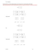
In the bases 3 and 4, the first of the two functions in each case is even under
P12 and the second is odd under P12 (immediately below we shall call these two
functions |ψ1 and |ψ2 ). Other operations give rise to a linear combination of the
two functions:
P12 |ψ1 = |ψ1 , P12 |ψ2 = − |ψ2 ,

(1.1.17a)

P13 |ψ1 = α11 |ψ1 + α12 |ψ2 , P13 |ψ2 = α21 |ψ1 + α22 |ψ2 ,

(1.1.17b)

with coefficients αij . In matrix form, (1.1.17b) can be written as
« „
«
„
«„
α11 α12
|ψ1
|ψ1
=
.

P13
|ψ2
|ψ2
α21 α22
The elements P12 and P13 are thus represented by 2 ì 2 matrices
ô

ô

1 0
11 12
.
P12 =
, P13 =
α21 α22
0 −1

(1.1.17c)

(1.1.18)

This fact implies that the basis vectors |ψ1 and |ψ2 span a two-dimensional representation of the permutation group S3 . The explicit calculation will be carried out
in Problem 1.2.

1.2 Completely Symmetric and Antisymmetric States
We begin with the single-particle states |i : |1 , |2 , . . . . The single-particle
states of the particles 1, 2, . . . , α, . . . , N are denoted by |i 1 , |i 2 , . . . , |i α ,
. . . , |i N . These enable us to write the basis states of the N -particle system
|i1 , . . . , iα , . . . , iN = |i1

1

. . . |iα

α

. . . |iN

N

,

(1.2.1)

where particle 1 is in state |i1 1 and particle α in state |iα α , etc. (The
subscript outside the ket is the number labeling the particle, and the index
within the ket identifies the state of this particle.)
Provided that the {|i } form a complete orthonormal set, the product
states defined above likewise represent a complete orthonormal system in the

www.pdfgrip.com


1.2 Completely Symmetric and Antisymmetric States

9

space of N -particle states. The symmetrized and antisymmetrized basis states
are then defined by
1

S± |i1 , i2 , . . . , iN ≡ √
N!

(±1)P P |i1 , i2 , . . . , iN .

(1.2.2)

P

In other words, we apply all N ! elements of the permutation group SN of N
objects and, for fermions, we multiply by (−1) when P is an odd permutation.
The states defined in (1.2.2) are of two types: completely symmetric and
completely antisymmetric.
Remarks regarding the properties of S± ≡

√1
N!

P
P (±1) P :

(i) Let SN be the permutation group (or symmetric group) of N quantities.
Assertion: For every element P ∈ SN , one has P SN = SN .
Proof. The set P SN contains exactly the same number of elements as SN and these,
due to the group property, are all contained in SN . Furthermore, the elements of
P SN are all different since, if one had P P1 = P P2 , then, after multiplication by
P −1 , it would follow that P1 = P2 .

Thus
P SN = SN P = SN .

(1.2.3)

(ii) It follows from this that
P S+ = S+ P = S+

(1.2.4a)

P S− = S− P = (−1)P S− .

(1.2.4b)

and

If P is even, then even elements remain even and odd ones remain odd. If
P is odd, then multiplication by P changes even into odd elements and vice
versa.
P S+ |i1 , . . . , iN = S+ |i1 , . . . , iN
P S− |i1 , . . . , iN = (−1)P S− |i1 , . . . , iN
Special case Pij S− |i1 , . . . , iN = −S− |i1 , . . . , iN .
(iii) If |i1 , . . . , iN contains single-particle states occurring more than once,
then S+ |i1 , . . . , iN is no longer normalized to unity. Let us assume that the
first state occurs n1 times, the second n2 times, etc. Since S+ |i1 , . . . , iN
N!
contains a total of N ! terms, of which n1 !n
are different, each of these
2 !...
terms occurs with a multiplicity of n1 !n2 ! . . . .
†
S+ |i1 , . . . , iN =

i 1 , . . . , i N | S+

N!
1
(n1 !n2 ! . . . )2
= n1 !n2 ! . . .
N!
n1 !n2 ! . . .

www.pdfgrip.com


10

1. Second Quantization

Thus, the normalized Bose basis functions are
1
1
S+ |i1 , . . . , iN √
= √
n1 !n2 ! . . .
N !n1 !n2 ! . . .

P |i1 , . . . , iN .

(1.2.5)

P

(iv) A further property of S± is
√
2
S±
= N !S± ,

(1.2.6a)

√
2
since S±
= √1N ! P (±1)P P S± = √1N ! P S± = N !S± . We now consider
an arbitrary N -particle state, which we expand in the basis |i1 . . . |iN
|z =

|i1 . . . |iN
i1 ,... ,iN

i1 , . . . , iN |z .
ci1 ,... ,iN

Application of S± yields
S± |z =

S± |i1 . . . |iN ci1 ,... ,iN =
i1 ,... ,iN

and further application of

|i1 . . . |iN S± ci1 ,... ,iN

i1 ,... ,iN

√1 S± ,
N!

with the identity (1.2.6a), results in

1
S± |z = √
S± |i1 . . . |iN (S± ci1 ,... ,iN ).
N ! i1 ,... ,iN

(1.2.6b)

Equation (1.2.6b) implies that every symmetrized state can be expanded in
terms of the symmetrized basis states (1.2.2).

1.3 Bosons
1.3.1 States, Fock Space, Creation and Annihilation Operators
The state (1.2.5) is fully characterized by specifying the occupation numbers
|n1 , n2 , . . . = S+ |i1 , i2 , . . . , iN √

1
.
n1 !n2 ! . . .

(1.3.1)

Here, n1 is the number of times that the state 1 occurs, n2 the number of
times that state 2 occurs, . . . . Alternatively: n1 is the number of particles in

state 1, n2 is the number of particles in state 2, . . . . The sum of all occupation
numbers ni must be equal to the total number of particles:
∞

ni = N.

(1.3.2)

i=1

www.pdfgrip.com


1.3 Bosons

11

Apart from this constraint, the ni can take any of the √values 0, 1, 2, . . . .
The factor (n1 !n2 ! . . . )−1/2 , together with the factor 1/ N ! contained in
S+ , has the effect of normalizing |n1 , n2 , . . . (see point (iii)). These states
form a complete set of completely symmetric N -particle states. By linear
superposition, one can construct from these any desired symmetric N -particle
state.
We now combine the states for N = 0, 1, 2, . . . and obtain a complete
orthonormal system of states for arbitrary particle number, which satisfy the
orthogonality relation6
n1 , n2 , . . . |n1 , n2 , . . . = δn1 ,n1 δn2 ,n2 . . .

(1.3.3a)

and the completeness relation
|n1 , n2 , . . . n1 , n2 , . . .| = 11 .

(1.3.3b)

n1 ,n2 ,...

This extended space is the direct sum of the space with no particles (vacuum
state |0 ), the space with one particle, the space with two particles, etc.; it is
known as Fock space.
The operators we have considered so far act only within a subspace of
fixed particle number. On applying p, x etc. to an N -particle state, we obtain
again an N -particle state. We now define creation and annihilation operators,
which lead from the space of N -particle states to the spaces of N ± 1-particle
states:
√
(1.3.4)
a†i |. . . , ni , . . . = ni + 1 |. . . , ni + 1, . . . .
Taking the adjoint of this equation and relabeling ni → ni , we have
. . . , ni , . . .| ai =

ni + 1 . . . , ni + 1, . . .| .

(1.3.5)

Multiplying this equation by |. . . , ni , . . . yields
√
. . . , ni , . . .| ai |. . . , ni , . . . = ni δni +1,ni .
Expressed in words, the operator ai reduces the occupation number by 1.
Assertion:

√
(1.3.6)
ai |. . . , ni , . . . = ni |. . . , ni − 1, . . . for ni ≥ 1
and
ai |. . . , ni = 0, . . . = 0 .
6

In the states |n1 , n2 , . . . , the n1 , n2 etc. are arbitrary natural numbers whose
sum is not constrained. The (vanishing) scalar product between states of differing
particle number is defined by (1.3.3a).

www.pdfgrip.com