Applied quantum mechanics 2nd edition

This page intentionally left blank

www.pdfgrip.com


Applied Quantum Mechanics, Second Edition
Electrical and mechanical engineers, materials scientists and applied physicists will find
Levi’s uniquely practical explanation of quantum mechanics invaluable. This updated
and expanded edition of the bestselling original text now covers quantization of angular
momentum and quantum communication, and problems and additional references are
included. Using real-world engineering examples to engage the reader, the author
makes quantum mechanics accessible and relevant to the engineering student. Numerous
illustrations, exercises, worked examples and problems are included; MATLAB® source
code to support the text is available from www.cambridge.org/9780521860963.
A. F. J. Levi is Professor of Electrical Engineering and of Physics and Astronomy at the
University of Southern California. He joined USC in 1993 after working for 10 years at
AT & T Bell Laboratories, New Jersey. He invented hot electron spectroscopy, discovered
ballistic electron transport in transistors, created the first microdisk laser, and carried out
groundbreaking work in parallel fiber optic interconnect components in computer and
switching systems. His current research interests include scaling of ultra-fast electronic
and photonic devices, system-level integration of advanced optoelectronic technologies,
manufacturing at the nanoscale, and the subject of Adaptive Quantum Design.

www.pdfgrip.com


www.pdfgrip.com


Applied Quantum Mechanics

Second Edition
A. F. J. Levi

www.pdfgrip.com


cambridge university press
Cambridge, New York, Melbourne, Madrid, Cape Town, Singapore, São Paulo
Cambridge University Press
The Edinburgh Building, Cambridge cb2 2ru, UK
Published in the United States of America by Cambridge University Press, New York
www.cambridge.org
Information on this title: www.cambridge.org/9780521860963
© Cambridge University Press 2006
This publication is in copyright. Subject to statutory exception and to the provision of
relevant collective licensing agreements, no reproduction of any part may take place
without the written permission of Cambridge University Press.
First published in print format 2006
isbn-13
isbn-10

978-0-511-19111-4 eBook (EBL)
0-511-19111-1 eBook (EBL)

isbn-13
isbn-10

978-0-521-86096-3 hardback
0-521-86096-2 hardback

Cambridge University Press has no responsibility for the persistence or accuracy of urls
for external or third-party internet websites referred to in this publication, and does not
guarantee that any content on such websites is, or will remain, accurate or appropriate.

www.pdfgrip.com


Dass ich erkenne, was die Welt
Im Innersten zusammenhält
Goethe
(Faust, I.382–3)

www.pdfgrip.com


www.pdfgrip.com


Contents

Preface to the first edition
Preface to the second edition
MATLAB® programs

page xiii
xv
xvi

1 Introduction
1.1 Motivation

1.2 Classical mechanics
1.2.1 Introduction
1.2.2 The one-dimensional simple harmonic oscillator
1.2.3 Harmonic oscillation of a diatomic molecule
1.2.4 The monatomic linear chain
1.2.5 The diatomic linear chain
1.3 Classical electromagnetism
1.3.1 Electrostatics
1.3.2 Electrodynamics
1.4 Example exercises
1.5 Problems

1
1
4
4
7
10
13
15
18
18
24
39
53

2 Toward quantum mechanics
2.1 Introduction
2.1.1 Diffraction and interference of light
2.1.2 Black-body radiation and evidence for quantization of light

2.1.3 Photoelectric effect and the photon particle
2.1.4 Secure quantum communication
2.1.5 The link between quantization of photons and other particles
2.1.6 Diffraction and interference of electrons
2.1.7 When is a particle a wave?
2.2 The Schrödinger wave equation
2.2.1 The wave function description of an electron in free space
2.2.2 The electron wave packet and dispersion
2.2.3 The hydrogen atom
2.2.4 Periodic table of elements
2.2.5 Crystal structure
2.2.6 Electronic properties of bulk semiconductors and heterostructures

57
57
58
62
64
66
70
71
72
73
79
80
83
89
93
96
vii

www.pdfgrip.com


CONTENTS

2.3
2.4

Example exercises
Problems

103
114

3 Using the Schrödinger wave equation
3.1 Introduction
3.1.1 The effect of discontinuity in the wave function and its slope
3.2 Wave function normalization and completeness
3.3 Inversion symmetry in the potential
3.3.1 One-dimensional rectangular potential well with infinite
barrier energy
3.4 Numerical solution of the Schrödinger equation
3.5 Current flow
3.5.1 Current in a rectangular potential well with infinite barrier
energy
3.5.2 Current flow due to a traveling wave
3.6 Degeneracy as a consequence of symmetry
3.6.1 Bound states in three dimensions and degeneracy of eigenvalues
3.7 Symmetric finite-barrier potential

3.7.1 Calculation of bound states in a symmetric finite-barrier
potential
3.8 Transmission and reflection of unbound states
3.8.1 Scattering from a potential step when m1 = m2
3.8.2 Scattering from a potential step when m1 = m2
3.8.3 Probability current density for scattering at a step
3.8.4 Impedance matching for unity transmission across a
potential step
3.9 Particle tunneling
3.9.1 Electron tunneling limit to reduction in size of CMOS
transistors
3.10 The nonequilibrium electron transistor
3.11 Example exercises
3.12 Problems

117
117
118
121
122

4 Electron propagation
4.1 Introduction
4.2 The propagation matrix method
4.3 Program to calculate transmission probability
4.4 Time-reversal symmetry
4.5 Current conservation and the propagation matrix
4.6 The rectangular potential barrier
4.6.1 Transmission probability for a rectangular potential barrier
4.6.2 Transmission as a function of energy

4.6.3 Transmission resonances
4.7 Resonant tunneling
4.7.1 Heterostructure bipolar transistor with resonant tunnel-barrier
4.7.2 Resonant tunneling between two quantum wells

171
171
172
177
178
180
182
182
185
186
188
190
192

viii

www.pdfgrip.com

123
126
128
129
131
131
131

133
135
137
138
140
141
142
145
149
150
155
168


CONTENTS

4.8
4.9

The potential barrier in the delta function limit
Energy bands in a periodic potential
4.9.1 Bloch’s Theorem
4.9.2 The propagation matrix applied to a periodic potential
4.9.3 The tight binding approximation
4.9.4 Crystal momentum and effective electron mass
Other engineering applications
The WKB approximation
4.11.1 Tunneling through a high-energy barrier of finite width
Example exercises
Problems

197
199
200
201
207
209
213
214
215
217
234

5 Eigenstates and operators
5.1 Introduction
5.1.1 The postulates of quantum mechanics
5.2 One-particle wave function space
5.3 Properties of linear operators
5.3.1 Product of operators
5.3.2 Properties of Hermitian operators
5.3.3 Normalization of eigenfunctions
5.3.4 Completeness of eigenfunctions
5.3.5 Commutator algebra
5.4 Dirac notation
5.5 Measurement of real numbers
5.5.1 Expectation value of an operator
5.5.2 Time dependence of expectation value
5.5.3 Uncertainty of expectation value
5.5.4 The generalized uncertainty relation
5.6 The no cloning theorem

5.7 Density of states
5.7.1 Density of electron states
5.7.2 Calculating density of states from a dispersion relation
5.7.3 Density of photon states
5.8 Example exercises
5.9 Problems

238
238
238
239
240
241
241
243
243
244
245
246
247
248
249
253
255
256
256
263
264
266
277

6 The harmonic oscillator
6.1 The harmonic oscillator potential
6.2 Creation and annihilation operators
6.2.1 The ground state of the harmonic oscillator
6.2.2 Excited states of the harmonic oscillator and normalization
of eigenstates
6.3 The harmonic oscillator wave functions
6.3.1 The classical turning point of the harmonic oscillator
6.4 Time dependence
6.4.1 The superposition operator

280
280
282
284

4.10
4.11
4.12
4.13

287
291
295
298
300
ix

www.pdfgrip.com

CONTENTS

6.4.2 Measurement of a superposition state
6.4.3 Time dependence of creation and annihilation operators
Quantization of electromagnetic fields
6.5.1 Laser light
6.5.2 Quantization of an electrical resonator
Quantization of lattice vibrations
Quantization of mechanical vibrations
Example exercises
Problems

300
301
305
306
306
307
308
309
323

7 Fermions and bosons
7.1 Introduction
7.1.1 The symmetry of indistinguishable particles
7.2 Fermi–Dirac distribution and chemical potential
7.2.1 Writing a computer program to calculate the chemical potential
7.2.2 Writing a computer program to plot the Fermi–Dirac distribution

7.2.3 Fermi–Dirac distribution function and thermal equilibrium
statistics
7.3 The Bose–Einstein distribution function
7.4 Example exercises
7.5 Problems

326
326
327
334
337
338

8 Time-dependent perturbation
8.1 Introduction
8.1.1 An abrupt change in potential
8.1.2 Time-dependent change in potential
8.2 First-order time-dependent perturbation
8.2.1 Charged particle in a harmonic potential
8.3 Fermi’s golden rule
8.4 Elastic scattering from ionized impurities
8.4.1 The coulomb potential
8.4.2 Linear screening of the coulomb potential
8.5 Photon emission due to electronic transitions
8.5.1 Density of optical modes in three-dimensions
8.5.2 Light intensity
8.5.3 Background photon energy density at thermal equilibrium
8.5.4 Fermi’s golden rule for stimulated optical transitions
8.5.5 The Einstein and coefficients
8.6 Example exercises

8.7 Problems

353
353
354
356
359
360
363
366
369
375
384
384
385
385
385
387
393
407

9 The semiconductor laser
9.1 Introduction
9.2 Spontaneous and stimulated emission
9.2.1 Absorption and its relation to spontaneous emission

412
412
413
416

6.5

6.6
6.7
6.8
6.9

x

www.pdfgrip.com

339
342
343
351


CONTENTS

9.3
9.4

9.5

9.6
9.7
9.8
9.9

Optical transitions using Fermi’s golden rule
9.3.1 Optical gain in the presence of electron scattering
Designing a laser diode
9.4.1 The optical cavity
9.4.2 Mirror loss and photon lifetime
9.4.3 The Fabry–Perot laser diode
9.4.4 Semiconductor laser diode rate equations
Numerical method of solving rate equations
9.5.1 The Runge–Kutta method
9.5.2 Large-signal transient response
9.5.3 Cavity formation
Noise in laser diode light emission
Why our model works
Example exercises
Problems

419
420
422
422
428
429
430
434
435
437
438
440
443
443

449

10 Time-independent perturbation
10.1 Introduction
10.2 Time-independent nondegenerate perturbation
10.2.1 The first-order correction
10.2.2 The second-order correction
10.2.3 Harmonic oscillator subject to perturbing potential in x
10.2.4 Harmonic oscillator subject to perturbing potential in x2
10.2.5 Harmonic oscillator subject to perturbing potential in x3
10.3 Time-independent degenerate perturbation
10.3.1 A two-fold degeneracy split by time-independent
perturbation
10.3.2 Matrix method
10.3.3 The two-dimensional harmonic oscillator subject to
perturbation in xy
10.3.4 Perturbation of two-dimensional potential with infinite
barrier energy
10.4 Example exercises
10.5 Problems

450
450
451
452
453
456
458
459
461

11 Angular momentum and the hydrogenic atom
11.1 Angular momentum
11.1.1 Classical angular momentum
11.2 The angular momentum operator
11.2.1 Eigenvalues of angular momentum operators Lˆ z and Lˆ 2
11.2.2 Geometrical representation
11.2.3 Spherical coordinates and spherical harmonics
11.2.4 The rigid rotator
11.3 The hydrogen atom
11.3.1 Eigenstates and eigenvalues of the hydrogen atom
11.3.2 Hydrogenic atom wave functions

485
485
485
487
489
491
492
498
499
500
508

462
462
465
467
471

482

xi

www.pdfgrip.com


CONTENTS

11.3.3 Electromagnetic radiation
11.3.4 Fine structure of the hydrogen atom and electron spin
11.4 Hybridization
11.5 Example exercises
11.6 Problems
Appendix A
Appendix B
Appendix C
Appendix D
Appendix E
Appendix F

Physical values
Coordinates, trigonometry, and mensuration
Expansions, differentiation, integrals, and mathematical relations
Matrices and determinants
Vector calculus and Maxwell’s equations
The Greek alphabet

Index

509
515
516
517
529
532
537
540
546
548
551
552

xii

www.pdfgrip.com


Preface to the first edition

The theory of quantum mechanics forms the basis for our present understanding of
physical phenomena on an atomic and sometimes macroscopic scale. Today, quantum
mechanics can be applied to most fields of science. Within engineering, important subjects
of practical significance include semiconductor transistors, lasers, quantum optics, and
molecular devices. As technology advances, an increasing number of new electronic
and opto-electronic devices will operate in ways which can only be understood using
quantum mechanics. Over the next thirty years, fundamentally quantum devices such as
single-electron memory cells and photonic signal processing systems may well become
commonplace. Applications will emerge in any discipline that has a need to understand,
control, and modify entities on an atomic scale. As nano- and atomic-scale structures

become easier to manufacture, increasing numbers of individuals will need to understand
quantum mechanics in order to be able to exploit these new fabrication capabilities. Hence,
one intent of this book is to provide the reader with a level of understanding and insight
that will enable him or her to make contributions to such future applications, whatever
they may be.
The book is intended for use in a one-semester introductory course in applied quantum
mechanics for engineers, material scientists, and others interested in understanding the
critical role of quantum mechanics in determining the behavior of practical devices. To
help maintain interest in this subject, I felt it was important to encourage the reader
to solve problems and to explore the possibilities of the Schrödinger equation. To ease
the way, solutions to example exercises are provided in the text, and the enclosed CDROM contains computer programs written in the MATLAB language that illustrate these
solutions. The computer programs may be usefully exploited to explore the effects of
changing parameters such as temperature, particle mass, and potential within a given
problem. In addition, they may be used as a starting point in the development of designs
for quantum mechanical devices.
The structure and content of this book are influenced by experience teaching the subject.
Surprisingly, existing texts do not seem to address the interests or build on the computing
skills of today’s students. This book is designed to better match such student needs.
Some material in the book is of a review nature, and some material is merely an
introduction to subjects that will undoubtedly be explored in depth by those interested
in pursuing more advanced topics. The majority of the text, however, is an essentially
self-contained study of quantum mechanics for electronic and opto-electronic applications.
xiii

www.pdfgrip.com


PREFACE TO THE FIRST EDITION

There are many important connections between quantum mechanics and classical

mechanics and electromagnetism. For this and other reasons, Chapter 1 is devoted to a
review of classical concepts. This establishes a point of view with which the predictions
of quantum mechanics can be compared. In a classroom situation it is also a convenient way in which to establish a uniform minimum knowledge base. In Chapter 2 the
Schrödinger wave equation is introduced and used to motivate qualitative descriptions
of atoms, semiconductor crystals, and a heterostructure diode. Chapter 3 develops the
more systematic use of the one-dimensional Schrödinger equation to describe a particle
in simple potentials. It is in this chapter that the quantum mechanical phenomenon of tunneling is introduced. Chapter 4 is devoted to developing and using the propagation matrix
method to calculate electron scattering from a one-dimensional potential of arbitrary
shape. Applications include resonant electron tunneling and the Kronig-Penney model
of a periodic crystal potential. The generality of the method is emphasized by applying
it to light scattering from a dielectric discontinuity. Chapter 5 introduces some related
mathematics, the generalized uncertainty relation, and the concept of density of states.
Following this, the quantization of conductance is introduced. The harmonic oscillator is
discussed in Chapter 6 using the creation and annihilation operators. Chapter 7 deals with
fermion and boson distribution functions. This chapter shows how to numerically calculate
the chemical potential for a multi-electron system. Chapter 8 introduces and then applies
time-dependent perturbation theory to ionized impurity scattering in a semiconductor and
spontaneous light-emission from an atom. The semiconductor laser diode is described in
Chapter 9. Finally, Chapter 10 discusses the (still useful) time-independent perturbation
theory.
Throughout this book, I have tried to make applications to systems of practical importance the main focus and motivation for the reader. Applications have been chosen because
of their dominant roles in today’s technologies. Understanding is, after all, only useful if
it can be applied.
A. F. J. Levi
2003

xiv

www.pdfgrip.com

Preface to the second edition

Following the remarkable success of the first edition and not wanting to give up on a
good thing, the second edition of this book continues to focus on three main themes:
practicing manipulation of equations and analytic problem solving in quantum mechanics,
utilizing the availability of modern compute power to numerically solve problems, and
developing an intuition for applications of quantum mechanics. Of course there are many
books which address the first of the three themes. However, the aim here is to go beyond
that which is readily available and provide the reader with a richer experience of the
possibilities of the Schrödinger equation and quantum phenomena.
Changes in the second edition include the addition of problems to each chapter. These
also appear on the Cambridge University Press website. To make space for these problems
and other additions, previously printed listing of MATLAB code has been removed from
the text. Chapter 1 now has a section on harmonic oscillation of a diatomic molecule.
Chapter 2 has a new section on quantum communication. In Chapter 3 the discussion of
numerical solutions to the Schrödinger now includes periodic boundary conditions. The
tight binding model of band structure has been added to Chapter 4 and the numerical
evaluation of density of states from dispersion relation has been added to Chapter 5.
The discussion of occupation number representation for electrons has been extended in
Chapter 7. Chapter 11 is a new chapter in which quantization of angular momentum and
the hydrogenic atom are introduced.
Cambridge University Press has a website with supporting material for both students
and teachers who use the book. This includes MATLAB code used to create figures and
solutions to exercises. The website is: />A. F. J. Levi
2006

xv

www.pdfgrip.com

MATLAB® programs

The computer requirements for the MATLAB1 language are an IBM or 100% compatible
system equipped with Intel 486, Pentium, Pentium Pro, Pentium4 processor or equivalent.
There should be an 8-bit or better graphics adapter and display, a minimum of 32 MB
RAM, and at least 50 MB disk space. The operating system should be Windows 95, NT4,
Windows 2000, or Windows XP.
If you have not already installed the MATLAB language on your computer, you
will need to purchase a copy and do so. MATLAB is available from MathWorks
( />After verifying correct installation of MATLAB, download the directory
AppliedQMmatlab from www.cambridge.org/9780521860963 and copy to a convenient
location in your computer user directory.
Launch MATLAB using the icon on the desktop or from the start menu. The MATLAB
command window will appear on your computer screen. From the MATLAB command
window use the path browser to set the path to the location of the AppliedQMmatlab
directory. Type the name of the file you wish to execute in the MATLAB command
window (do not include the “.m” extension). Press the enter key on the keyboard to run
the program.
You will find that some programs prompt for input from the keyboard. Most programs
display results graphically with intermediate results displayed in the MATLAB command
window.
To edit values in a program or to edit the program itself double-click on the file name
to open the file editor.
You should note that the computer programs in the AppliedQMmatlab directory are
not optimized. They are written in a very simple way to minimize any possible confusion
or sources of error. The intent is that these programs be used as an aid to the study of
applied quantum mechanics. When required, integration is performed explicitly, and in
the simplest way possible. However, for exercises involving matrix diagonalization use

is made of special MATLAB functions.
Some programs make use of the functions chempot.m, fermi.m, mu.m, runge4.m, and
solve_schM.m, and Chapt9Exercise5.m reads data from the datainLI.txt data input file.

1. MATLAB is a registered trademark of MathWorks, Inc.

xvi

www.pdfgrip.com


1

Introduction

1.1 Motivation
You may ask why one needs to know about
quantum mechanics. Possibly the simplest
answer is that we live in a quantum world!
Engineers would like to make and control electronic, opto-electronic, and optical devices on an atomic scale. In biology there are molecules and cells we wish
to understand and modify on an atomic
scale. The same is true in chemistry, where
an important goal is the synthesis of both
organic and inorganic compounds with
precise atomic composition and structure.
Quantum mechanics gives the engineer, the
biologist, and the chemist the tools with
which to study and control objects on an
atomic scale.
As an example, consider the deoxyribonucleic acid (DNA) molecule shown in

Fig. 1.1. The number of atoms in DNA can
be so great that it is impossible to track the
position and activity of every atom. However, suppose we wish to know the effect a
particular site (or neighborhood of an atom)
in a single molecule has on a chemical
reaction. Making use of quantum mechanics, engineers, biologists, and chemists can
work together to solve this problem. In one
approach, laser-induced fluorescence of a
fluorophore attached to a specific site of
a large molecule can be used to study the
dynamics of that individual molecule. The
light emitted from the fluorophore acts as
a small beacon that provides information
about the state of the molecule. This technique, which relies on quantum mechanical

S

C

N

O

Fig. 1.1 Ball and stick model of a DNA molecule.
Atom types are indicated.

1

www.pdfgrip.com

INTRODUCTION

photon stimulation and photon emission from atomic states, has been used to track the
behavior of single DNA molecules.1
Interdisciplinary research that uses quantum mechanics to study and control the behavior of atoms is, in itself, a very interesting subject. However, even within a given discipline
such as electrical engineering, there are important reasons to study quantum mechanics.
In the case of electrical engineering, one simple motivation is the fact that transistor
dimensions will soon approach a size where single-electron and quantum effects determine device performance. Over the last few decades advances in the complexity and
performance of complementary metal-oxide-semiconductor (CMOS) circuits have been
carefully managed by the microelectronics industry to follow what has become known
as “Moore’s Law.”2 This rule-of-thumb states that the number of transistors in silicon
integrated circuits increases by a factor of two every eighteen months. Associated with
this law is an increase in the performance of computers. The Semiconductor Industry
Association (SIA) has institutionalized Moore’s Law via the “SIA Roadmap,” which
tracks and identifies advances needed in most of the electronics industry’s technologies.3
Remarkably, reductions in the size of transistors and related technology have allowed
Moore’s Law to be sustained for over 35 years (see Fig. 1.2). Nevertheless, the impossibility of continued reduction in transistor device dimensions is well illustrated by the
fact that Moore’s law predicts that dynamic random access memory (DRAM) cell size
will be less than that of an atom by the year 2030. Well before this end-point is reached,
quantum effects will dominate device performance, and conventional electronic circuits
will fail to function.

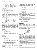
Fig. 1.2 Photograph (left) of the first transistor. Brattain and Bardeen’s p-n-p point-contact germanium transistor operated as a speech amplifier with a power gain of 18 on December 23, 1947. The device is a few mm
in size. On the right is a scanning capacitance microscope cross-section image of a silicon p-type metal-oxidesemiconductor field-effect transistor (p-MOSFET) with an effective channel length of about 20 nm, or about 60
atoms.4 This image of a small transistor was published in 1998, 50 years after Brattain and Bardeen’s device.
Image courtesy of G. Timp, University of Illinois.
1. S. Weiss, Science 283, 1676 (1999).
2. G. E. Moore, Electronics 38, 114 (1965). Also reprinted in Proc. IEEE 86, 82 (1998).
3. .

4. Also see G. Timp et al. IEEE International Electron Devices Meeting (IEDM) Technical Digest p. 615, Dec.
6–9, San Francisco, California, 1998 (ISBN 078034779).

2

www.pdfgrip.com


1.1 MOTIVATION

We need to learn to use quantum mechanics to make sure that we can create the
smallest, highest-performance devices possible.
Quantum mechanics is the basis for our present understanding of physical phenomena
on an atomic scale. Today, quantum mechanics has numerous applications in engineering,
including semiconductor transistors, lasers, and quantum optics. As technology advances,
an increasing number of new electronic and opto-electronic devices will operate in ways
that can only be understood using quantum mechanics. Over the next 20 years, fundamentally quantum devices such as single-electron memory cells and photonic signal processing
systems may well become commonplace. It is also likely that entirely new devices, with
functionality based on the principles of quantum mechanics, will be invented. The purpose
and intent of this book is to provide the reader with a level of understanding and insight
that will enable him or her to appreciate and to make contributions to the development of
these future, as yet unknown, applications of quantum phenomena.
The small glimpse of our quantum world that this book provides reveals significant
differences from our everyday experience. Often we will discover that the motion of
objects does not behave according to our (classical) expectations. A simple, but hopefully
motivating, example is what happens when you throw a ball against a wall. Of course,
we expect the ball to bounce right back. Quantum mechanics has something different
to say. There is, under certain special circumstances, a finite chance that the ball will
appear on the other side of the wall! This effect, known as tunneling, is fundamentally
quantum mechanical and arises due to the fact that on appropriate time and length

scales particles can be described as waves. Situations in which elementary particles
such as electrons and photons tunnel are, in fact, relatively common. However, quantum
mechanical tunneling is not always limited to atomic-scale and elementary particles.
Tunneling of large (macroscopic) objects can also occur! Large objects, such as a ball,
are made up of many atomic-scale particles. The possibility that such large objects can
tunnel is one of the more amazing facts that emerges as we explore our quantum world.
However, before diving in and learning about quantum mechanics it is worth spending
a little time and effort reviewing some of the basics of classical mechanics and classical
electromagnetics. We do this in the next two sections. The first deals with classical
mechanics, which was first placed on a solid theoretical basis by the work of Newton and
Leibniz published at the end of the seventeenth century. The survey includes reminders
about the concepts of potential and kinetic energy and the conservation of energy in
a closed system. The important example of the one-dimensional harmonic oscillator is
then considered. The simple harmonic oscillator is extended to the case of the diatomic
linear chain, and the concept of dispersion is introduced. Going beyond mechanics, in the
following section classical electromagnetism is explored. We start by stating the coulomb
potential for charged particles, and then we use the equations that describe electrostatics to
solve practical problems. The classical concepts of capacitance and the coulomb blockade
are used as examples. Continuing our review, Maxwell’s equations are used to study
electrodynamics. The first example discussed is electromagnetic wave propagation at the
speed of light in free space, c. The key result – that power and momentum are carried by
an electromagnetic wave – is also introduced.
Following our survey of classical concepts, in Chapter 2 we touch on the experimental
basis for quantum mechanics. This includes observation of the interference phenomenon
with light, which is described in terms of the linear superposition of waves. We then
3

www.pdfgrip.com

INTRODUCTION

discuss the important early work aimed at understanding the measured power spectrum of
black-body radiation as a function of wavelength, , or frequency, = 2 c/ . Next, we
treat the photoelectric effect, which is best explained by requiring that light be quantized
into particles (called photons) of energy E = . Planck’s constant = 1 0545 × 10−34 J s,
which appears in the expression E =
, is a small number that sets the absolute scale
for which quantum effects usually dominate behavior.5 Since the typical length scale for
which electron energy quantization is important usually turns out to be the size of an
atom, the observation of discrete spectra for light emitted from excited atoms is an effect
that can only be explained using quantum mechanics. The energy of photons emitted from
excited hydrogen atoms is discussed in terms of the solutions of the Schrödinger equation.
Because historically the experimental facts suggested a wave nature for electrons, the
relationships among the wavelength, energy, and momentum of an electron are introduced.
This section concludes with some examples of the behavior of electrons, including the
description of an electron in free space, the concept of a wave packet and dispersion of a
wave packet, and electronic configurations for atoms in the ground state.
Since we will later apply our knowledge of quantum mechanics to semiconductors and
semiconductor devices, there is also a brief introduction to crystal structure, the concept
of a semiconductor energy band gap, and the device physics of a unipolar heterostructure
semiconductor diode.
1.2
1.2.1

Classical mechanics
Introduction

The problem classical mechanics sets out to solve is predicting the motion of large
(macroscopic) objects. On the face of it, this could be a very difficult subject simply

because large objects tend to have a large number of degrees of freedom6 and so, in
principle, should be described by a large number of parameters. In fact, the number of
parameters could be so enormous as to be unmanageable. The remarkable success of
classical mechanics is due to the fact that powerful concepts can be exploited to simplify
the problem. Constants of the motion and constraints may be used to reduce the description
of motion to a simple set of differential equations. Examples of constants of the motion
often include conservation of energy and momentum.7 Describing an object as rigid is an
example of a constraint being placed on the object.
Consider a rock dropped from a tower. Classical mechanics initially ignores the internal
degrees of freedom of the rock (it is assumed to be rigid), but instead defines a center of
mass so that the rock can be described as a point particle of mass, m. Angular momentum
is decoupled from the center of mass motion. Why is this all possible? The answer is
neither simple nor obvious.
5. Sometimes

is called Planck’s reduced constant to distinguish it from h = 2

.

6. For example, an object may be able to vibrate in many different ways.
7. Emmy Noether showed in 1915 that the existence of a symmetry due to a local interaction gives rise to a
conserved quantity. For example, conservation of energy is due to time translation symmetry, conservation
of linear momentum is due to space translational symmetry, and angular momentum conservation is due to
rotational symmetry.

4

www.pdfgrip.com

1.2 CLASSICAL MECHANICS

It is known from experiments that atomic-scale particle motion can be very different
from the predictions of classical mechanics. Because large objects are made up of many
atoms, one approach is to suggest that quantum effects are somehow averaged out in
large objects. In fact, classical mechanics is often assumed to be the macroscopic (largescale) limit of quantum mechanics. The underlying notion of finding a means to link
quantum mechanics to classical mechanics is so important it is called the correspondence
principle. Formally, one requires that the results of classical mechanics be obtained in
the limit → 0. While a simple and convenient test, this approach misses the point. The
results of classical mechanics are obtained because the quantum mechanical wave nature
of objects is averaged out by a mechanism called decoherence. In this picture, quantum
mechanical effects are usually averaged out in large objects to give the classical result.
However, this is not always the case. We should remember that sometimes even large
(macroscopic) objects can show quantum effects. A well-known example of a macroscopic
quantum effect is superconductivity and the tunneling of flux quanta in a device called a
SQUID.8 The tunneling of flux quanta is the quantum-mechanical equivalent of throwing
a ball against a wall and having it sometimes tunnel through to the other side! Quantum
mechanics allows large objects to tunnel through a thin potential barrier if the constituents
of the object are prepared in a special quantum-mechanical state. The wave nature of the
entire object must be maintained if it is to tunnel through a potential barrier. One way to
achieve this is to have a coherent superposition of constituent particle wave functions.
Returning to classical mechanics, we can now say that the motion of macroscopic
material bodies is usually described by classical mechanics. In this approach, the linear
momentum of a rigid object with mass m is p = m dx/dt, where v = dx/dt is the velocity
of the object moving in the direction of the unit vector x∼ = x/ x . Time is measured
in units of seconds (s), and distance is measured in units of meters (m). The magnitude
of momentum is measured in units of kilogram meters per second (kg m s−1 ), and the
magnitude of velocity (speed) is measured in units of meters per second (m s−1 ). Classical
mechanics assumes that there exists an inertial frame of reference for which the motion
of the object is described by the differential equation

F = dp/dt = m d2 x/dt2

(1.1)

where the vector F is the force. The magnitude of force is measured in units of newtons
(N). Force is a vector field. What this means is that the particle can be subject to a force
the magnitude and direction of which are different in different parts of space.
We need a new concept to obtain a measure of the forces experienced by the particle
moving from position r1 to r2 in space. The approach taken is to introduce the idea of
work. The work done moving the object from point 1 to point 2 in space along a path is
defined as
r=r2

W12 =

F · dr

(1.2)

r=r1

8. For an introduction to this see A. J. Leggett, Physics World 12, 73 (1999).

5

www.pdfgrip.com


INTRODUCTION

r = r2

r = r1
Fig. 1.3

Illustration of a classical particle trajectory from position r1 to r2 .

where r is a spatial vector coordinate. Figure 1.3 illustrates one possible trajectory for a
particle moving from position r1 to r2 .
The definition of work is simply the integral of the force applied multiplied by the
infinitesimal distance moved in the direction of the force for the complete path from point 1
to point 2. For a conservative force field, the work W12 is the same for any path between
points 1 and 2. Hence, making use of the fact F = dp/dt = m dv/dt, one may write
r=r2

W12 =

F · dr = m

r=r1

dv/dt · vdt =

m
2

d
dt

2

dt

(1.3)

so that W12 = m 22 − 12 /2 = T2 − T1 , where 2 = v · v and the scalar T = m 2 /2 is
called the kinetic energy of the object.
For conservative forces, because the work done is the same for any path between
points 1 and 2, the work done around any closed path, such as the one illustrated in
Fig. 1.4, is always zero, or
F · dr = 0

(1.4)

This is always true if force is the gradient of a single-valued spatial scalar field where
F=− V r

(1.5)

since F · dr = −
V · dr = − dV = 0. In our expression, V r is called the potential.
Potential is measured in volts (V), and potential energy is measured in joules (J) or
electron volts (eV). If the forces acting on the object are conservative, then total energy,
which is the sum of kinetic and potential energy, is a constant of the motion. In other
words, total energy T + V is conserved.
Since kinetic and potential energy can be expressed as functions of the variable’s
position and time, it is possible to define a Hamiltonian function for the system, which
is H = T + V . The Hamiltonian function may then be used to describe the dynamics of
particles in the system.
For a nonconservative force, such as a particle subject to frictional forces, the work

done around any closed path is not zero, and F · dr = 0.

Fig. 1.4

Illustration of a closed-path classical particle trajectory.

6

www.pdfgrip.com


1.2 CLASSICAL MECHANICS

Let us pause here for a moment and consider some of what has just been introduced.
We think of objects moving due to something. Forces cause objects to move. We have
introduced the concept of force to help ensure that the motion of objects can be described
as a simple process of cause and effect. We imagine a force-field in three-dimensional
space that is represented mathematically as a continuous, integrable vector field, F r .
Assuming that time is also continuous and integrable, we quickly discover that in a
conservative force-field energy is conveniently partitioned between a kinetic and potential
term and total energy is conserved. By simply representing the total energy as a function or
Hamiltonian, H = T + V , we can find a differential equation that describes the dynamics
of the object. Integration of the differential equation of motion gives the trajectory of the
object as it moves through space.
In practice, these ideas are very powerful and may be applied to many problems
involving the motion of macroscopic objects. As an example, let us consider the problem
of finding the motion of a particle mass, m, attached to a spring. Of course, we know
from experience that the solution will be oscillatory and so characterized by a frequency
and amplitude of oscillation. However, the power of the theory is that we can obtain
relationships among all the parameters that govern the behavior of the system.

In the next section, the motion of a classical particle mass m attached to a spring
and constrained to move in one dimension is discussed. The type of model we will be
considering is called the simple harmonic oscillator.
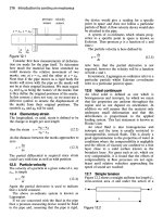
1.2.2

The one-dimensional simple harmonic oscillator

Figure 1.5 illustrates a classical particle mass m constrained to motion in one dimension
and attached to a lightweight spring that obeys Hooke’s law. Hooke’s law states that the
displacement, x, from the equilibrium position, x = 0, is proportional to the force on the
particle such that F = − x where the proportionality constant is and is called the spring
constant. In this example, we ignore any effect due to the finite mass of the spring by
assuming its mass is small relative to the particle mass, m.
To calculate the frequency and amplitude of vibration, we start by noting that the total
energy function or Hamiltonian for the system is
H = T +V

(1.6)

Force, F = –κ x
Spring constant, κ

Mass, m

Closed system with no exchange
of energy outside the system
implies conservation of energy

Displacement, x
Fig. 1.5 Illustration showing a classical particle mass m attached to a spring and constrained to move in one

dimension. The displacement of the particle from its equilibrium position is x and the force on the particle is
F = − x where is the spring constant The box drawn with a broken line indicates a closed system.

7

www.pdfgrip.com