- Trang chủ >>
- Khoa Học Tự Nhiên >>
- Vật lý
Many body quantum theory in condensed matter physics
Bạn đang xem bản rút gọn của tài liệu. Xem và tải ngay bản đầy đủ của tài liệu tại đây (3.4 MB, 352 trang )
Introduction to
Many-body quantum theory in
condensed matter physics
Henrik Bruus and Karsten Flensberg
Ørsted Laboratory, Niels Bohr Institute, University of Copenhagen
Mikroelektronik Centret, Technical University of Denmark
Copenhagen, 15 August 2002
www.pdfgrip.com
ii
www.pdfgrip.com
Preface
Preface for the 2001 edition
This introduction to quantum field theory in condensed matter physics has emerged from
our courses for graduate and advanced undergraduate students at the Niels Bohr Institute,
University of Copenhagen, held between the fall of 1999 and the spring of 2001. We have
gone through the pain of writing these notes, because we felt the pedagogical need for
a book which aimed at putting an emphasis on the physical contents and applications
of the rather involved mathematical machinery of quantum field theory without loosing
mathematical rigor. We hope we have succeeded at least to some extend in reaching this
goal.
We would like to thank the students who put up with the first versions of this book and
for their enumerable and valuable comments and suggestions. We are particularly grateful
to the students of Many-particle Physics I & II, the academic year 2000-2001, and to Niels
Asger Mortensen and Brian Møller Andersen for careful proof reading. Naturally, we are
solely responsible for the hopefully few remaining errors and typos.
During the work on this book H.B. was supported by the Danish Natural Science Research Council through Ole Rømer Grant No. 9600548.
Ørsted Laboratory, Niels Bohr Institute
1 September, 2001
Karsten Flensberg
Henrik Bruus
Preface for the 2002 edition
After running the course in the academic year 2001-2002 our students came up with more
corrections and comments so that we felt a new edition was appropriate. We would like
to thank our ever enthusiastic students for their valuable help in improving this book.
Karsten Flensberg
Ørsted Laboratory
Niels Bohr Institute
Henrik Bruus
Mikroelektronik Centret
Technical University of Denmark
iii
www.pdfgrip.com
iv
PREFACE
www.pdfgrip.com
Contents
List of symbols
xii
1 First and second quantization
1.1 First quantization, single-particle systems . . . . . . . . . . . .
1.2 First quantization, many-particle systems . . . . . . . . . . . .
1.2.1 Permutation symmetry and indistinguishability . . . . .
1.2.2 The single-particle states as basis states . . . . . . . . .
1.2.3 Operators in first quantization . . . . . . . . . . . . . .
1.3 Second quantization, basic concepts . . . . . . . . . . . . . . .
1.3.1 The occupation number representation . . . . . . . . . .
1.3.2 The boson creation and annihilation operators . . . . .
1.3.3 The fermion creation and annihilation operators . . . .
1.3.4 The general form for second quantization operators . . .
1.3.5 Change of basis in second quantization . . . . . . . . . .
1.3.6 Quantum field operators and their Fourier transforms .
1.4 Second quantization, specific operators . . . . . . . . . . . . . .
1.4.1 The harmonic oscillator in second quantization . . . . .
1.4.2 The electromagnetic field in second quantization . . . .
1.4.3 Operators for kinetic energy, spin, density, and current .
1.4.4 The Coulomb interaction in second quantization . . . .
1.4.5 Basis states for systems with different kinds of particles
1.5 Second quantization and statistical mechanics . . . . . . . . . .
1.5.1 The distribution function for non-interacting fermions .
1.5.2 Distribution functions for non-interacting bosons . . . .
1.6 Summary and outlook . . . . . . . . . . . . . . . . . . . . . . .
2 The electron gas
2.1 The non-interacting electron gas . . . . . . . . . . . . . . . .
2.1.1 Bloch theory of electrons in a static ion lattice . . . .
2.1.2 Non-interacting electrons in the jellium model . . . . .
2.1.3 Non-interacting electrons at finite temperature . . . .
2.2 Electron interactions in perturbation theory . . . . . . . . . .
2.2.1 Electron interactions in 1st order perturbation theory
v
.
.
.
.
.
.
.
.
.
.
.
.
.
.
.
.
.
.
.
.
.
.
.
.
.
.
.
.
.
.
.
.
.
.
.
.
.
.
.
.
.
.
.
.
.
.
.
.
.
.
.
.
.
.
.
.
.
.
.
.
.
.
.
.
.
.
.
.
.
.
.
.
.
.
.
.
.
.
.
.
.
.
.
.
.
.
.
.
.
.
.
.
.
.
.
.
.
.
.
.
.
.
.
.
.
.
.
.
.
.
.
.
.
.
.
.
.
.
.
.
.
.
.
.
.
.
.
.
.
.
.
.
.
.
.
.
.
.
.
.
.
.
.
.
.
.
.
.
.
.
.
.
.
.
.
.
.
.
.
.
.
.
.
.
.
.
.
.
.
.
.
.
.
.
.
.
.
.
.
.
.
.
.
.
.
.
.
.
.
.
.
.
.
.
.
.
1
2
4
5
6
7
9
10
10
13
14
16
17
18
18
19
21
23
24
25
28
29
29
.
.
.
.
.
.
31
32
33
35
38
39
41
www.pdfgrip.com
vi
CONTENTS
2.2.2 Electron interactions in 2nd order perturbation theory .
Electron gases in 3, 2, 1, and 0 dimensions . . . . . . . . . . . .
2.3.1 3D electron gases: metals and semiconductors . . . . . .
2.3.2 2D electron gases: GaAs/Ga1−x Alx As heterostructures .
2.3.3 1D electron gases: carbon nanotubes . . . . . . . . . . .
2.3.4 0D electron gases: quantum dots . . . . . . . . . . . . .
.
.
.
.
.
.
.
.
.
.
.
.
.
.
.
.
.
.
.
.
.
.
.
.
.
.
.
.
.
.
.
.
.
.
.
.
.
.
.
.
.
.
43
44
45
46
48
49
.
.
.
.
.
.
.
.
.
.
.
.
.
.
.
.
.
.
.
.
.
.
.
.
.
.
.
.
.
.
.
.
.
.
.
.
.
.
.
.
.
.
.
.
.
.
.
.
.
.
.
.
.
.
.
.
51
52
53
53
56
59
61
63
64
4 Mean field theory
4.1 The art of mean field theory . . . . . . . . . . . . . . . . . . . . .
4.2 Hartree–Fock approximation . . . . . . . . . . . . . . . . . . . . .
4.3 Broken symmetry . . . . . . . . . . . . . . . . . . . . . . . . . . .
4.4 Ferromagnetism . . . . . . . . . . . . . . . . . . . . . . . . . . . .
4.4.1 The Heisenberg model of ionic ferromagnets . . . . . . . .
4.4.2 The Stoner model of metallic ferromagnets . . . . . . . .
4.5 Superconductivity . . . . . . . . . . . . . . . . . . . . . . . . . .
4.5.1 Breaking of global gauge symmetry and its consequences .
4.5.2 Microscopic theory . . . . . . . . . . . . . . . . . . . . . .
4.6 Summary and outlook . . . . . . . . . . . . . . . . . . . . . . . .
.
.
.
.
.
.
.
.
.
.
.
.
.
.
.
.
.
.
.
.
.
.
.
.
.
.
.
.
.
.
.
.
.
.
.
.
.
.
.
.
.
.
.
.
.
.
.
.
.
.
.
.
.
.
.
.
.
.
.
.
65
68
69
71
73
73
75
78
78
81
85
5 Time evolution pictures
5.1 The Schrăodinger picture . . . . . . . . . . . . . . . .
5.2 The Heisenberg picture . . . . . . . . . . . . . . . .
5.3 The interaction picture . . . . . . . . . . . . . . . . .
5.4 Time-evolution in linear response . . . . . . . . . . .
5.5 Time dependent creation and annihilation operators
5.6 Summary and outlook . . . . . . . . . . . . . . . . .
2.3
3 Phonons; coupling to electrons
3.1 Jellium oscillations and Einstein phonons . . . . .
3.2 Electron-phonon interaction and the sound velocity
3.3 Lattice vibrations and phonons in 1D . . . . . . .
3.4 Acoustical and optical phonons in 3D . . . . . . .
3.5 The specific heat of solids in the Debye model . . .
3.6 Electron-phonon interaction in the lattice model .
3.7 Electron-phonon interaction in the jellium model .
3.8 Summary and outlook . . . . . . . . . . . . . . . .
.
.
.
.
.
.
.
.
.
.
.
.
.
.
.
.
.
.
.
.
.
.
.
.
.
.
.
.
.
.
.
.
.
.
.
.
.
.
.
.
.
.
.
.
.
.
.
.
.
.
.
.
.
.
.
.
.
.
.
.
.
.
.
.
.
.
.
.
.
.
.
.
.
.
.
.
.
.
.
.
.
.
.
.
.
.
.
.
.
.
.
.
.
.
.
.
.
.
.
.
.
.
.
.
.
.
.
.
.
.
87
87
88
88
91
91
93
6 Linear response theory
6.1 The general Kubo formula . . . . . . . . . . . . . . . . . . . .
6.2 Kubo formula for conductivity . . . . . . . . . . . . . . . . .
6.3 Kubo formula for conductance . . . . . . . . . . . . . . . . .
6.4 Kubo formula for the dielectric function . . . . . . . . . . . .
6.4.1 Dielectric function for translation-invariant system . .
6.4.2 Relation between dielectric function and conductivity
.
.
.
.
.
.
.
.
.
.
.
.
.
.
.
.
.
.
.
.
.
.
.
.
.
.
.
.
.
.
.
.
.
.
.
.
.
.
.
.
.
.
.
.
.
.
.
.
95
95
98
100
102
104
104
.
.
.
.
.
.
.
.
.
.
.
.
.
.
.
.
.
.
.
.
.
.
.
.
www.pdfgrip.com
CONTENTS
6.5
vii
Summary and outlook . . . . . . . . . . . . . . . . . . . . . . . . . . . . . . 104
7 Transport in mesoscopic systems
7.1 The S-matrix and scattering states . . . . . . . . . . . . . . . . . .
7.1.1 Unitarity of the S-matrix . . . . . . . . . . . . . . . . . . .
7.1.2 Time-reversal symmetry . . . . . . . . . . . . . . . . . . . .
7.2 Conductance and transmission coefficients . . . . . . . . . . . . . .
7.2.1 The Landauer-Bă
uttiker formula, heuristic derivation . . . .
7.2.2 The Landauer-Bă
uttiker formula, linear response derivation .
7.3 Electron wave guides . . . . . . . . . . . . . . . . . . . . . . . . . .
7.3.1 Quantum point contact and conductance quantization . . .
7.3.2 Aharonov-Bohm effect . . . . . . . . . . . . . . . . . . . . .
7.4 Disordered mesoscopic systems . . . . . . . . . . . . . . . . . . . .
7.4.1 Statistics of quantum conductance, random matrix theory .
7.4.2 Weak localization in mesoscopic systems . . . . . . . . . . .
7.4.3 Universal conductance fluctuations . . . . . . . . . . . . . .
7.5 Summary and outlook . . . . . . . . . . . . . . . . . . . . . . . . .
.
.
.
.
.
.
.
.
.
.
.
.
.
.
.
.
.
.
.
.
.
.
.
.
.
.
.
.
.
.
.
.
.
.
.
.
.
.
.
.
.
.
.
.
.
.
.
.
.
.
.
.
.
.
.
.
107
. 108
. 111
. 112
. 113
. 113
. 115
. 116
. 116
. 120
. 121
. 121
. 123
. 124
. 125
8 Green’s functions
8.1 “Classical” Green’s functions . . . . . . . . . . . . . . . .
8.2 Green’s function for the one-particle Schrăodinger equation
8.3 Single-particle Greens functions of many-body systems .
8.3.1 Green’s function of translation-invariant systems .
8.3.2 Green’s function of free electrons . . . . . . . . . .
8.3.3 The Lehmann representation . . . . . . . . . . . .
8.3.4 The spectral function . . . . . . . . . . . . . . . .
8.3.5 Broadening of the spectral function . . . . . . . . .
8.4 Measuring the single-particle spectral function . . . . . .
8.4.1 Tunneling spectroscopy . . . . . . . . . . . . . . .
8.4.2 Optical spectroscopy . . . . . . . . . . . . . . . . .
8.5 Two-particle correlation functions of many-body systems .
8.6 Summary and outlook . . . . . . . . . . . . . . . . . . . .
.
.
.
.
.
.
.
.
.
.
.
.
.
.
.
.
.
.
.
.
.
.
.
.
.
.
.
.
.
.
.
.
.
.
.
.
.
.
.
.
.
.
.
.
.
.
.
.
.
.
.
.
.
.
.
.
.
.
.
.
.
.
.
.
.
127
127
128
131
132
132
134
135
136
137
137
141
141
144
9 Equation of motion theory
9.1 The single-particle Green’s function . . . . . . . . . . . . . . . . . . .
9.1.1 Non-interacting particles . . . . . . . . . . . . . . . . . . . . . .
9.2 Anderson’s model for magnetic impurities . . . . . . . . . . . . . . . .
9.2.1 The equation of motion for the Anderson model . . . . . . . .
9.2.2 Mean-field approximation for the Anderson model . . . . . . .
9.2.3 Solving the Anderson model and comparison with experiments
9.2.4 Coulomb blockade and the Anderson model . . . . . . . . . . .
9.2.5 Further correlations in the Anderson model: Kondo effect . . .
9.3 The two-particle correlation function . . . . . . . . . . . . . . . . . . .
9.3.1 The Random Phase Approximation (RPA) . . . . . . . . . . .
.
.
.
.
.
.
.
.
.
.
.
.
.
.
.
.
.
.
.
.
.
.
.
.
.
.
.
.
.
.
145
145
147
147
149
150
151
153
153
153
153
.
.
.
.
.
.
.
.
.
.
.
.
.
.
.
.
.
.
.
.
.
.
.
.
.
.
.
.
.
.
.
.
.
.
.
.
.
.
.
.
.
.
.
.
.
.
.
.
.
.
.
.
.
.
.
.
.
.
.
.
.
.
.
.
.
www.pdfgrip.com
viii
CONTENTS
9.4
Summary and outlook . . . . . . . . . . . . . . . . . . . . . . . . . . . . . . 156
10 Imaginary time Green’s functions
10.1 Definitions of Matsubara Green’s functions . . . . . . . . . . .
10.1.1 Fourier transform of Matsubara Green’s functions . . .
10.2 Connection between Matsubara and retarded functions . . . . .
10.2.1 Advanced functions . . . . . . . . . . . . . . . . . . . .
10.3 Single-particle Matsubara Green’s function . . . . . . . . . . .
10.3.1 Matsubara Green’s function for non-interacting particles
10.4 Evaluation of Matsubara sums . . . . . . . . . . . . . . . . . .
10.4.1 Summations over functions with simple poles . . . . . .
10.4.2 Summations over functions with known branch cuts . .
10.5 Equation of motion . . . . . . . . . . . . . . . . . . . . . . . . .
10.6 Wick’s theorem . . . . . . . . . . . . . . . . . . . . . . . . . . .
10.7 Example: polarizability of free electrons . . . . . . . . . . . . .
10.8 Summary and outlook . . . . . . . . . . . . . . . . . . . . . . .
.
.
.
.
.
.
.
.
.
.
.
.
.
.
.
.
.
.
.
.
.
.
.
.
.
.
.
.
.
.
.
.
.
.
.
.
.
.
.
.
.
.
.
.
.
.
.
.
.
.
.
.
.
.
.
.
.
.
.
.
.
.
.
.
.
.
.
.
.
.
.
.
.
.
.
.
.
.
157
. 160
. 161
. 161
. 163
. 164
. 164
. 165
. 167
. 168
. 169
. 170
. 173
. 174
11 Feynman diagrams and external potentials
11.1 Non-interacting particles in external potentials . . . . . . .
11.2 Elastic scattering and Matsubara frequencies . . . . . . . .
11.3 Random impurities in disordered metals . . . . . . . . . . .
11.3.1 Feynman diagrams for the impurity scattering . . .
11.4 Impurity self-average . . . . . . . . . . . . . . . . . . . . . .
11.5 Self-energy for impurity scattered electrons . . . . . . . . .
11.5.1 Lowest order approximation . . . . . . . . . . . . . .
11.5.2 1st order Born approximation . . . . . . . . . . . . .
11.5.3 The full Born approximation . . . . . . . . . . . . .
11.5.4 The self-consistent Born approximation and beyond
11.6 Summary and outlook . . . . . . . . . . . . . . . . . . . . .
.
.
.
.
.
.
.
.
.
.
.
.
.
.
.
.
.
.
.
.
.
.
.
.
.
.
.
.
.
.
.
.
.
.
.
.
.
.
.
.
.
.
.
.
.
.
.
.
.
.
.
.
.
.
.
.
.
.
.
.
.
.
.
.
.
.
.
.
.
.
.
.
.
.
.
.
.
.
.
.
.
.
.
.
.
.
.
.
177
. 177
. 179
. 181
. 182
. 184
. 189
. 190
. 190
. 193
. 194
. 197
12 Feynman diagrams and pair interactions
12.1 The perturbation series for G . . . . . . . . . . . . . . . . .
12.2 infinite perturbation series!Matsubara Green’s function . . .
12.3 The Feynman rules for pair interactions . . . . . . . . . . .
12.3.1 Feynman rules for the denominator of G(b, a) . . . .
12.3.2 Feynman rules for the numerator of G(b, a) . . . . .
12.3.3 The cancellation of disconnected Feynman diagrams
12.4 Self-energy and Dyson’s equation . . . . . . . . . . . . . . .
12.5 The Feynman rules in Fourier space . . . . . . . . . . . . .
12.6 Examples of how to evaluate Feynman diagrams . . . . . .
12.6.1 The Hartree self-energy diagram . . . . . . . . . . .
12.6.2 The Fock self-energy diagram . . . . . . . . . . . . .
12.6.3 The pair-bubble self-energy diagram . . . . . . . . .
12.7 Summary and outlook . . . . . . . . . . . . . . . . . . . . .
.
.
.
.
.
.
.
.
.
.
.
.
.
.
.
.
.
.
.
.
.
.
.
.
.
.
.
.
.
.
.
.
.
.
.
.
.
.
.
.
.
.
.
.
.
.
.
.
.
.
.
.
.
.
.
.
.
.
.
.
.
.
.
.
.
.
.
.
.
.
.
.
.
.
.
.
.
.
.
.
.
.
.
.
.
.
.
.
.
.
.
.
.
.
.
.
.
.
.
.
.
.
.
.
.
.
.
.
.
.
.
.
.
.
.
.
.
199
199
199
201
201
202
203
205
206
208
209
209
210
211
www.pdfgrip.com
CONTENTS
13 The interacting electron gas
13.1 The self-energy in the random phase approximation .
13.1.1 The density dependence of self-energy diagrams
13.1.2 The divergence number of self-energy diagrams
13.1.3 RPA resummation of the self-energy . . . . . .
13.2 The renormalized Coulomb interaction in RPA . . . .
13.2.1 Calculation of the pair-bubble . . . . . . . . . .
13.2.2 The electron-hole pair interpretation of RPA .
13.3 The ground state energy of the electron gas . . . . . .
13.4 The dielectric function and screening . . . . . . . . . .
13.5 Plasma oscillations and Landau damping . . . . . . .
13.5.1 Plasma oscillations and plasmons . . . . . . . .
13.5.2 Landau damping . . . . . . . . . . . . . . . . .
13.6 Summary and outlook . . . . . . . . . . . . . . . . . .
ix
.
.
.
.
.
.
.
.
.
.
.
.
.
.
.
.
.
.
.
.
.
.
.
.
.
.
.
.
.
.
.
.
.
.
.
.
.
.
.
.
.
.
.
.
.
.
.
.
.
.
.
.
.
.
.
.
.
.
.
.
.
.
.
.
.
.
.
.
.
.
.
.
.
.
.
.
.
.
.
.
.
.
.
.
.
.
.
.
.
.
.
.
.
.
.
.
.
.
.
.
.
.
.
.
.
.
.
.
.
.
.
.
.
.
.
.
.
.
.
.
.
.
.
.
.
.
.
.
.
.
.
.
.
.
.
.
.
.
.
.
.
.
.
213
. 213
. 214
. 215
. 215
. 217
. 218
. 220
. 220
. 223
. 227
. 228
. 230
. 231
14 Fermi liquid theory
14.1 Adiabatic continuity . . . . . . . . . . . . . . . . . . . . . . .
14.1.1 The quasiparticle concept and conserved quantities . .
14.2 Semi-classical treatment of screening and plasmons . . . . . .
14.2.1 Static screening . . . . . . . . . . . . . . . . . . . . . .
14.2.2 Dynamical screening . . . . . . . . . . . . . . . . . . .
14.3 Semi-classical transport equation . . . . . . . . . . . . . . . .
14.3.1 Finite life time of the quasiparticles . . . . . . . . . .
14.4 Microscopic basis of the Fermi liquid theory . . . . . . . . . .
14.4.1 Renormalization of the single particle Green’s function
14.4.2 Imaginary part of the single particle Green’s function
14.4.3 Mass renormalization? . . . . . . . . . . . . . . . . . .
14.5 Outlook and summary . . . . . . . . . . . . . . . . . . . . . .
.
.
.
.
.
.
.
.
.
.
.
.
.
.
.
.
.
.
.
.
.
.
.
.
.
.
.
.
.
.
.
.
.
.
.
.
.
.
.
.
.
.
.
.
.
.
.
.
.
.
.
.
.
.
.
.
.
.
.
.
.
.
.
.
.
.
.
.
.
.
.
.
.
.
.
.
.
.
.
.
.
.
.
.
233
. 233
. 235
. 237
. 238
. 238
. 240
. 243
. 245
. 245
. 248
. 251
. 251
15 Impurity scattering and conductivity
15.1 Vertex corrections and dressed Green’s functions . . .
15.2 The conductivity in terms of a general vertex function
15.3 The conductivity in the first Born approximation . . .
15.4 The weak localization correction to the conductivity .
15.5 Combined RPA and Born approximation . . . . . . . .
.
.
.
.
.
.
.
.
.
.
.
.
.
.
.
.
.
.
.
.
.
.
.
.
.
.
.
.
.
.
.
.
.
.
.
.
.
.
.
.
.
.
.
.
.
.
.
275
. 275
. 276
. 279
. 279
. 280
. 281
. 284
.
.
.
.
.
.
.
.
.
.
.
.
.
.
.
.
.
.
.
.
16 Green’s functions and phonons
16.1 The Green’s function for free phonons . . . . . . . . . . . . . . . . . .
16.2 Electron-phonon interaction and Feynman diagrams . . . . . . . . . .
16.3 Combining Coulomb and electron-phonon interactions . . . . . . . . .
16.3.1 Migdal’s theorem . . . . . . . . . . . . . . . . . . . . . . . . . .
16.3.2 Jellium phonons and the effective electron-electron interaction
16.4 Phonon renormalization by electron screening in RPA . . . . . . . . .
16.5 The Cooper instability and Feynman diagrams . . . . . . . . . . . . .
.
.
.
.
.
.
.
253
254
259
261
264
273
www.pdfgrip.com
x
17 Superconductivity
17.1 The Cooper instability . . . . . . . . .
17.2 The BCS groundstate . . . . . . . . .
17.3 BCS theory with Green’s functions . .
17.4 Experimental consequences of the BCS
17.4.1 Tunneling density of states . .
17.4.2 specific heat . . . . . . . . . . .
17.5 The Josephson effect . . . . . . . . . .
CONTENTS
.
.
.
.
.
.
.
.
.
.
.
.
.
.
.
.
.
.
.
.
.
.
.
.
.
.
.
.
.
.
.
.
.
.
.
.
.
.
.
.
.
.
.
.
.
.
.
.
.
.
.
.
.
.
.
.
.
.
.
.
.
.
.
.
.
.
.
.
.
.
.
.
.
.
.
.
.
287
. 287
. 287
. 287
. 288
. 288
. 288
. 288
18 1D electron gases and Luttinger liquids
18.1 Introduction . . . . . . . . . . . . . . . . . . . . . . . . .
18.2 First look at interacting electrons in one dimension . . .
18.2.1 One-dimensional transmission line analog . . . .
18.3 The Luttinger-Tomonaga model - spinless case . . . . .
18.3.1 Interacting one dimensional electron system . . .
18.3.2 Bosonization of Tomonaga model-Hamiltonian .
18.3.3 Diagonalization of bosonized Hamiltonian . . . .
18.3.4 Real space formulation . . . . . . . . . . . . . . .
18.3.5 Electron operators in bosonized form . . . . . . .
18.4 Luttinger liquid with spin . . . . . . . . . . . . . . . . .
18.5 Green’s functions . . . . . . . . . . . . . . . . . . . . . .
18.6 Tunneling into spinless Luttinger liquid . . . . . . . . .
18.6.1 Tunneling into the end of Luttinger liquid . . . .
18.7 What is a Luttinger liquid? . . . . . . . . . . . . . . . .
18.8 Experimental realizations of Luttinger liquid physics . .
18.8.1 Edge states in the fractional quantum Hall effect
18.8.2 Carbon Nanotubes . . . . . . . . . . . . . . . . .
.
.
.
.
.
.
.
.
.
.
.
.
.
.
.
.
.
.
.
.
.
.
.
.
.
.
.
.
.
.
.
.
.
.
.
.
.
.
.
.
.
.
.
.
.
.
.
.
.
.
.
.
.
.
.
.
.
.
.
.
.
.
.
.
.
.
.
.
.
.
.
.
.
.
.
.
.
.
.
.
.
.
.
.
.
.
.
.
.
.
.
.
.
.
.
.
.
.
.
.
.
.
.
.
.
.
.
.
.
.
.
.
.
.
.
.
.
.
.
.
.
.
.
.
.
.
.
.
.
.
.
.
.
.
.
.
.
.
.
.
.
.
.
.
.
.
.
.
.
.
.
.
.
.
.
.
.
.
.
.
.
.
.
.
.
.
.
.
.
.
.
.
.
.
.
.
.
.
.
.
.
.
.
.
.
.
.
289
289
289
289
289
289
289
289
289
289
290
290
290
290
290
290
290
290
A Fourier transformations
A.1 Continuous functions in a finite region . .
A.2 Continuous functions in an infinite region
A.3 Time and frequency Fourier transforms .
A.4 Some useful rules . . . . . . . . . . . . . .
A.5 Translation invariant systems . . . . . . .
.
.
.
.
.
.
.
.
.
.
.
.
.
.
.
.
.
.
.
.
.
.
.
.
.
.
.
.
.
.
.
.
.
.
.
.
.
.
.
.
.
.
.
.
.
.
.
.
.
.
.
.
.
.
.
291
291
292
292
292
293
. . . .
. . . .
. . . .
states
. . . .
. . . .
. . . .
.
.
.
.
.
.
.
.
.
.
.
.
.
.
.
.
.
.
.
.
.
.
.
.
.
.
.
.
.
.
.
.
.
.
.
.
.
.
.
.
.
.
.
.
.
.
.
.
.
.
.
.
.
.
.
.
.
.
.
.
.
.
.
.
.
.
.
.
.
.
.
.
.
.
.
B Exercises
295
C Index
326
www.pdfgrip.com
List of symbols
Symbol
Meaning
Definition
ˆ
♥
Sec. 5.3
|ν
ν|
|0
operator ♥ in the interaction picture
time derivative of ♥
Dirac ket notation for a quantum state ν
Dirac bra notation for an adjoint quantum state ν
vacuum state
a
a†
aν , a†ν
a±
n
a0
A(r, t)
A(ν, ω)
A(r, ω), A(k, ω)
A0 (r, ω), A0 (k, ω)
A, A†
annihilation operator for particle (fermion or boson)
creation operator for particle (fermion or boson)
annihilation/creation operators (state ν)
amplitudes of wavefunctions to the left
Bohr radius
electromagnetic vector potential
spectral function in frequency domain (state ν)
spectral function (real space, Fourier space)
spectral function for free particles
phonon annihilation and creation operator
b
b†
b±
n
B
annihilation operator for particle (boson, phonon)
creation operator for particle (boson, phonon)
amplitudes of wavefunctions to the right
magnetic field
c
c†
cν , c†ν
R (t, t )
CAB
A (t, t )
CAB
R
CII (ω)
CAB
C(Q, ikn , ikn + iqn )
C R (Q, ε, ε)
CVion
annihilation operator for particle (fermion, electron)
creation operator for particle (fermion, electron)
annihilation/creation operators (state ν)
retarded correlation function between A and B (time)
advanced correlation function between A and B (time)
retarded current-current correlation function (frequency)
Matsubara correlation function
Cooperon in the Matsubara domain
Cooperon in the real time domain
specific heat for ions (constant volume)
˙
♥
xi
Chap. 1
Chap. 1
Sec. 7.1
Eq. (2.36)
Sec. 1.4.2
Sec. 8.3.4
Sec. 8.3.4
Sec. 8.3.4
Sec. 16.1
Sec. 7.1
Sec.
Sec.
Sec.
Sec.
Sec.
Sec.
6.1
10.2.1
6.3
10.1
15.4
15.4
www.pdfgrip.com
xii
LIST OF SYMBOLS
Symbol
Meaning
Definition
d( )
δ(r)
DR (rt, rt )
DR (q, ω)
D(rτ, rτ )
D(q, iqn )
DR (νt, ν t )
Dαβ (r)
∆k
density of states (including spin degeneracy for electrons)
Dirac delta function
retarded phonon propagator
retarded phonon propagator (Fourier space)
Matsubara phonon propagator
Matsubara phonon propagator (Fourier space)
retarded many particle Green’s function
phonon dynamical matrix
superconducting orderparameter
Eq. (2.31)
Eq. (1.11)
Chap. 16
Chap. 16
Chap. 16
Chap. 16
Eq. (9.9b)
Sec. 3.4)
Eq. (4.58b)
e
e20
E(r, t)
E
E (1)
E (2)
E0
Ek
ε
ε(rt, rt )
ε(k, ω)
elementary charge
electron interaction strength
electric field
total energy of the electron gas
interaction energy of the electron gas, 1st order perturbation
interaction energy of the electron gas, 2nd order perturbation
Rydberg energy
dispersion relation for BCS quasiparticles
energy variable
the dielectric constant of vacuum
dispersion relation
energy of quantum state ν
Fermi energy
phonon polarization vector
dielectric function in real space
dielectric function in Fourier space
F
|FS
φ(r, t)
φext
φind
φ, φ˜
±
φ±
LnE , φRnE
free energy
the filled Fermi sea N -particle quantum state
electric potential
external electric potential
induced electric potential
wavefunctions with different normalizations
wavefunctions in the left and right leads
gqλ
gq
G
electron-phonon coupling constant (lattice model)
electron-phonon coupling constant (jellium model)
conductance
0
εk
εν
εF
kλ
Eq. (1.101)
Eq. (2.36)
Eq. (4.64)
Eq. (3.20)
Sec. 6.4
Sec. 6.4
Sec. 1.5
Eq. (7.4)
Sec. 7.1
www.pdfgrip.com
LIST OF SYMBOLS
xiii
Symbol
Meaning
Definition
G(rt, r t )
G0 (rt, r t )
G<
0 (rt, r t )
G>
0 (rt, r t )
GA
0 (rt, r t )
GR
0 (rt, r t )
GR
0 (k, ω)
G< (rt, r t )
G> (rt, r t )
GA (rt, r t )
GR (rt, r t )
GR (k, ω)
GR (k, ω)
GR (νt, ν t )
G(rστ, r σ τ )
G(ντ, ν τ )
G(1, 1 )
˜ k˜ )
G(k,
G0 (rστ, r σ τ )
G0 (ντ, ν τ )
G0 (k, ikn )
G0 (ν, ikn )
(n)
G0
G(k, ikn )
G(ν, ikn )
γ, γ RA
Γ
˜ k˜ + q˜)
Γx (k,
Γ0,x
Green’s function for the Schrăodinger equation
unperturbed Greens function for Schrăodingers eq.
free lesser Greens function
free grater Green’s function
free advanced Green’s function
free retarded Green’s function
free retarded Green’s function (Fourier space)
lesser Green’s function
greater Green’s function
advanced Green’s function
retarded Green’s function (real space)
retarded Green’s function in Fourier space
retarded Green’s function (Fourier space)
retarded single-particle Green’s function ({ν} basis)
Matsubara Green’s function (real space)
Matsubara Green’s function ({ν} basis)
Matsubara Green’s function (real space four-vectors)
Matsubara Green’s function (four-momentum notation)
Matsubara Green’s function (real space, free particles)
Matsubara Green’s function ({ν} basis, free particles)
Matsubara Green’s function (Fourier space, free particles)
Matsubara Green’s function (free particles )
n-particle Green’s function (free particles)
Matsubara Green’s function (Fourier space)
Matsubara Green’s function ({ν} basis, frequency domain)
scalar vertex function
imaginary part of self-energy
vertex function (x-component, four vector notation)
free (undressed) vertex function
Sec. 8.2
Sec. 8.2
Sec. 8.3.1
Sec. 8.3.1
Sec. 8.3.1
Sec. 8.3.1
Sec. 8.3.1
Sec. 8.3
Sec. 8.3
Sec. 8.3
Sec. 8.3
Sec. 8.3
Sec. 8.3.1
Eq. (8.32)
Sec. 10.3
Sec. 10.3
Sec. 11.1
Sec. 12.5
Sec. 10.3.1
Sec. 10.3.1
Sec. 10.3
Sec. 10.3
Sec. 10.6
Sec. 10.3
Sec. 10.3
Sec. 15.3
H
H0
H
Hext
Hint
Hph
η
a general Hamiltonian
unperturbed part of an Hamiltonian
perturbative part of an Hamiltonian
external potential part of an Hamiltonian
interaction part of an Hamiltonian
phonon part of an Hamiltonian
positive infinitisimal
I
Ie
current operator (particle current)
electrical current (charge current)
Eq. (15.20b)
Sec. 6.3
Sec. 6.3
www.pdfgrip.com
xiv
LIST OF SYMBOLS
Symbol
Meaning
Definition
Jσ (r)
Jσ∆ (r)
JσA (r)
Jσ (q)
Je (r, t)
Jij
current density operator
current density operator, paramagnetic term
current density operator, diamagnetic term
current density operator (momentum space)
electric current density operator
interaction strength in the Heisenberg model
Eq. (1.99a)
Eq. (1.99a)
Eq. (1.99a)
kn
kF
k
Matsubara frequency (fermions)
Fermi wave number
general momentum or wave vector variable
L
λF
Λirr
mean free path or scattering length
mean free path (first Born approximation)
phase breaking mean free path
inelastic scattering length
normalization length or system size in 1D
Fermi wave length
irreducible four-point function
m
m∗
µ
µ
mass (electrons and general particles)
effective interaction renormalized mass
chemical potential
general quantum number label
n
nF (ε)
nB (ε)
nimp
N
Nimp
ν
particle density
Fermi-Dirac distribution function
Bose-Einstein distribution function
impurity density
number of particles
number of impurities
general quantum number label
ω
ωq
ωn
Ω
frequency variable
phonon dispersion relation
Matsubara frequency
thermodynamic potential
p
pn
ΠR
αβ (rt, r t )
R
Παβ (q, ω)
Παβ (q, iωn )
Π0 (q, iqn )
general momentum or wave number variable
Matsubara frequency (fermion)
retarded current-current correlation function
retarded current-current correlation function
Matsubara current-current correlation function
free pair-bubble diagram
0
φ
in
Sec. 4.4.1
Eq. (15.17)
Sec. 14.4.1
Sec. 1.5.1
Sec. 1.5.2
Chap. 10
Sec. 1.5
Eq. (6.26)
Chap. 15
Eq. (12.34)
www.pdfgrip.com
LIST OF SYMBOLS
Symbol
Meaning
q
qn
general momentum variable
Matsubara frequency (bosons)
r
r
r
rs
ρ
ρ0
ρσ (r)
ρσ (q)
general space variable
reflection matrix coming from left
reflection matrix coming from right
electron gas density parameter
density matrix
unperturbed density matrix
particle density operator (real space)
particle density opetor (momentum space)
S
S
σ
σαβ (rt, r t )
ΣR (q, ω)
Σ(q, ikn )
Σk
Σ1BA
k
ΣFBA
k
ΣSCBA
k
Σ(l, j)
Σσ (k, ikn )
ΣFσ (k, ikn )
ΣH
σ (k, ikn )
ΣPσ (k, ikn )
ΣRPA
(k, ikn )
σ
entropy
scattering matrix
general spin index
conductivity tensor
retarded self-energy (Fourier space)
Matsubara self-energy
impurity scattering self-energy
first Born approximation
full Born approximation
self-consistent Born approximation
general electron self-energy
general electron self-energy
Fock self-energy
Hartree self-energy
pair-bubble self-energy
RPA electron self-energy
t
t
t
T
τ
τ tr
τ0 , τk
general time variable
tranmission matrix coming from left
transmission matrix coming from right
kinetic energy
general imaginary time variable
transport scattering time
life-time in the first Born approximation
uj
u(R0 )
uk
U
ˆ (t, t )
U
ˆ (τ, τ )
U
ion displacement (1D)
ion displacement (3D)
BCS coherence factor
general unitary matrix
real time-evolution operator, interaction picture
imaginary time-evolution operator, interaction picture
xv
Definition
Sec. 7.1
Sec. 7.1
Eq. (2.37)
Sec. 1.5
Eq. (1.96)
Eq. (1.96)
Sec. 7.1
Sec. 6.2
Sec.
Sec.
Sec.
Sec.
11.5
11.5.1
11.5.3
11.5.4
Sec. 12.6
Sec. 12.6
Sec. 12.6
Eq. (13.10)
Sec. 7.1
Sec. 7.1
Eq. (14.39)
Sec. 4.5.2
www.pdfgrip.com
xvi
LIST OF SYMBOLS
Symbol
Meaning
Definition
vk
V (r), V (q)
V (r), V (q)
Veff
V
BCS coherence factor
general single impurity potential
Coulomb interaction
combined Coulomb and phonon-mediated interaction
normalization volume
Sec. 4.5.2
W
W (r), W (q)
W (r), W (q)
W RPA
pair interaction Hamiltonian
general pair interaction
Coulomb interaction
RPA-screened Coulomb interaction
ξk
ξν
χ(q, iqn )
χRPA (q, iqn )
χirr (q, iqn )
χ0 (rt, r t )
χ0 (q, iqn )
χR (rt, r t )
χR (q, ω)
χn (y)
εk − µ
εν − µ
Matsubara charge-charge correlation function
RPA Matsubara charge-charge correlation function
irreducible Matsubara charge-charge correlation function
free retarded charge-charge correlation function
free Matsubara charge-charge correlation function
retarded charge-charge correlation function
retarded charge-charge correlation function (Fourier)
transverse wavefunction
ψν (r)
±
ψnE
ψ(r1 , r2 , . . . , rn )
Ψσ (r)
Ψ†σ (r)
single-particle wave function, quantum number ν
single-particle scattering states
n-particle wave function (first quantization)
quantum field annihilation operator
quantum field creation operator
θ(x)
Heaviside’s step function
Sec. 13.2
Sec. 13.2
Sec. 13.4
Sec. 13.4
Sec. 13.4
Sec. 13.4
Eq. (6.39)
Sec. 7.1
Sec. 7.1
Sec. 1.3.6
Sec. 1.3.6
Eq. (1.12)
www.pdfgrip.com
Chapter 1
First and second quantization
Quantum theory is the most complete microscopic theory we have today describing the
physics of energy and matter. It has successfully been applied to explain phenomena
ranging over many orders of magnitude, from the study of elementary particles on the
sub-nucleonic scale to the study of neutron stars and other astrophysical objects on the
cosmological scale. Only the inclusion of gravitation stands out as an unsolved problem
in fundamental quantum theory.
Historically, quantum physics first dealt only with the quantization of the motion of
particles leaving the electromagnetic field classical, hence the name quantum mechanics
(Heisenberg, Schrăodinger, and Dirac 1925-26). Later also the electromagnetic field was
quantized (Dirac, 1927), and even the particles themselves got represented by quantized
fields (Jordan and Wigner, 1928), resulting in the development of quantum electrodynamics (QED) and quantum field theory (QFT) in general. By convention, the original form of
quantum mechanics is denoted first quantization, while quantum field theory is formulated
in the language of second quantization.
Regardless of the representation, be it first or second quantization, certain basic concepts are always present in the formulation of quantum theory. The starting point is
the notion of quantum states and the observables of the system under consideration.
Quantum theory postulates that all quantum states are represented by state vectors in
a Hilbert space, and that all observables are represented by Hermitian operators acting
on that space. Parallel state vectors represent the same physical state, and one therefore
mostly deals with normalized state vectors. Any given Hermitian operator A has a number
of eigenstates |ψα that up to a real scale factor α is left invariant by the action of the
operator, A|ψα = α|ψα . The scale factors are denoted the eigenvalues of the operator.
It is a fundamental theorem of Hilbert space theory that the set of all eigenvectors of any
given Hermitian operator forms a complete basis set of the Hilbert space. In general the
eigenstates |ψα and |φβ of two different Hermitian operators A and B are not the same.
By measurement of the type B the quantum state can be prepared to be in an eigenstate
|φβ of the operator B. This state can also be expressed as a superposition of eigenstates
|ψα of the operator A as |φβ = α |ψα Cαβ . If one in this state measures the dynamical
variable associated with the operator A, one cannot in general predict the outcome with
1
www.pdfgrip.com
2
CHAPTER 1. FIRST AND SECOND QUANTIZATION
certainty. It is only described in probabilistic terms. The probability of having any given
|ψα as the outcome is given as the absolute square |Cαβ |2 of the associated expansion
coefficient. This non-causal element of quantum theory is also known as the collapse of
the wavefunction. However, between collapse events the time evolution of quantum states
is perfectly deterministic. The time evolution of a state vector |ψ(t) is governed by the
central operator in quantum mechanics, the Hamiltonian H (the operator associated with
the total energy of the system), through Schrăodingers equation
i ∂t |ψ(t) = H|ψ(t) .
(1.1)
Each state vector |ψ is associated with an adjoint state vector (|ψ )† ≡ ψ|. One can
form inner products, “bra(c)kets”, ψ|φ between adjoint “bra” states ψ| and “ket” states
|φ , and use standard geometrical terminology, e.g. the norm squared of |ψ is given by
ψ|ψ , and |ψ and |φ are said to be orthogonal if ψ|φ = 0. If {|ψα } is an orthonormal
basis of the Hilbert space, then the above mentioned expansion coefficient Cαβ is found
by forming inner products: Cαβ = ψα |φβ . A further connection between the direct and
the adjoint Hilbert space is given by the relation ψ|φ = φ|ψ ∗ , which also leads to the
definition of adjoint operators. For a given operator A the adjoint operator A† is defined
by demanding ψ|A† |φ = φ|A|ψ ∗ for any |ψ and |φ .
In this chapter we will briefly review standard first quantization for one and manyparticle systems. For more complete reviews the reader is refereed to the textbooks by
Dirac, Landau and Lifshitz, Merzbacher, or Shankar. Based on this we will introduce
second quantization. This introduction is not complete in all details, and we refer the
interested reader to the textbooks by Mahan, Fetter and Walecka, and Abrikosov, Gorkov,
and Dzyaloshinskii.
1.1
First quantization, single-particle systems
For simplicity consider a non-relativistic particle, say an electron with charge −e, moving
in an external electromagnetic field described by the potentials ϕ(r, t) and A(r, t). The
corresponding Hamiltonian is
H=
1
2m
2
i
∇r + eA(r, t)
− eϕ(r, t).
(1.2)
An eigenstate describing a free spin-up electron travelling inside a box of volume V
can be written as a product of a propagating plane wave and a spin-up spinor. Using the
Dirac notation the state ket can be written as |ψk,↑ = |k, ↑ , where one simply lists the
relevant quantum numbers in the ket. The state function (also denoted the wave function)
and the ket are related by
ψk,σ (r) = r|k, σ = √1V eik·r χσ
(free particle orbital),
(1.3)
i.e. by the inner product of the position bra r| with the state ket.
The plane wave representation |k, σ is not always a useful starting point for calculations. For example in atomic physics, where electrons orbiting a point-like positively
www.pdfgrip.com
1.1. FIRST QUANTIZATION, SINGLE-PARTICLE SYSTEMS
✁
✂
✄
✂
☎
3
✂
Figure 1.1: The probability density | r|ψν |2 in the xy plane for (a) any plane wave
ν = (kx , ky , kz , σ), (b) the hydrogen orbital ν = (4, 2, 0, σ), and (c) the Landau orbital
ν = (3, ky , 0, σ).
charged nucleus are considered, the hydrogenic eigenstates |n, l, m, σ are much more useful. Recall that
r|n, l, m, σ = Rnl (r)Yl,m (θ, φ)χσ
(hydrogen orbital), ,
(1.4)
where Rnl (r) is a radial Coulomb function with n−l nodes, while Yl,m (θ, φ) is a spherical
harmonic representing angular momentum l with a z component m.
A third example is an electron moving in a constant magnetic field B = B ez , which
in the Landau gauge A = xB ey leads to the Landau eigenstates |n, ky , kz , σ , where n is
an integer, ky (kz ) is the y (z) component of k, and σ the spin variable. Recall that
1
r|n, ky , kz , σ = Hn (x/ −ky )e− 2 (x/
−ky )2 √
1
Ly Lz
ei(ky y+kz z) χσ
(Landau orbital), , (1.5)
where =
/eB is the magnetic length and Hn is the normalized Hermite polynomial
of order n associated with the harmonic oscillator potential induced by the magnetic field.
Examples of each of these three types of electron orbitals are shown in Fig. 1.1.
In general a complete set of quantum numbers is denoted ν . The three examples
given above corresponds to ν = (kx , ky , kz , σ), ν = (n, l, m, σ), and ν = (n, ky , kz , σ) each
yielding a state function of the form ψν (r) = r|ν . The completeness of a basis state
as well as the normalization of the state vectors play a central role in quantum theory.
Loosely speaking the normalization condition means that with probability unity a particle
in a given quantum state ψν (r) must be somewhere in space: dr |ψν (r)|2 = 1, or in the
Dirac notation: 1 = dr ν|r r|ν = ν| ( dr |r r|) |ν . From this we conclude
dr |r r| = 1.
(1.6)
Similarly, the completeness of a set of basis states ψν (r) means that if a particle is in
some state ψ(r) it must be found with probability unity within the orbitals of the basis
2
set:
ν | ν|ψ | = 1. Again using the Dirac notation we find 1 =
ν ψ|ν ν|ψ =
ψ| ( ν |ν ν|) |ψ , and we conclude
|ν ν| = 1.
ν
(1.7)
www.pdfgrip.com
4
CHAPTER 1. FIRST AND SECOND QUANTIZATION
We shall often use the completeness relation Eq. (1.7). A simple example is the expansion
of a state function in a given basis: ψ(r) = r|ψ = r|1|ψ = r| ( ν |ν ν|) |ψ =
ν r|ν ν|ψ , which can be expressed as
ψ(r) =
dr ψν∗ (r )ψ(r )
ψν (r)
or
r|ψ =
ν
r|ν ν|ψ .
(1.8)
ν
It should be noted that the quantum label ν can contain both discrete and continuous
quantum numbers. In that case the symbol ν is to be interpreted as a combination
of both summations and integrations. For example in the case in Eq. (1.5) with Landau
orbitals in a box with side lengths Lx , Ly , and Lz , we have
∞
=
ν
σ=↑,↓ n=0
∞
Ly
dky
−∞ 2π
∞
Lz
dkz .
−∞ 2π
(1.9)
In the mathematical formulation of quantum theory we shall often encounter the following special functions.
Kronecker’s delta-function δk,n for discrete variables,
δk,n =
1, for k = n,
0, for k = n.
(1.10)
Dirac’s delta-function δ(r) for continuous variables,
δ(r) = 0, for r = 0,
while
dr δ(r) = 1,
(1.11)
and Heaviside’s step-function θ(x) for continuous variables,
θ(x) =
1.2
0, for x < 0,
1, for x > 0.
(1.12)
First quantization, many-particle systems
When turning to N -particle systems, i.e. a system containing N identical particles, say,
electrons, three more assumptions are added to the basic assumptions defining quantum
theory. The first assumption is the natural extension of the single-particle state function
ψ(r), which (neglecting the spin degree of freedom for the time being) is a complex wave
function in 3-dimensional space, to the N -particle state function ψ(r1 , r2 , . . . , rN ), which
is a complex function in the 3N -dimensional configuration space. As for one particle this
N -particle state function is interpreted as a probability amplitude such that its absolute
square is related to a probability:
The probability for finding the N particles
N
in the 3N −dimensional volume N
drj
2
j=1
|ψ(r1 , r2 , . . . , rN )|
(1.13)
drj =
surrounding the point (r1 , r2 , . . . , rN ) in
j=1
the 3N −dimensional configuration space.
www.pdfgrip.com
1.2. FIRST QUANTIZATION, MANY-PARTICLE SYSTEMS
1.2.1
5
Permutation symmetry and indistinguishability
A fundamental difference between classical and quantum mechanics concerns the concept
of indistinguishability of identical particles. In classical mechanics each particle can be
equipped with an identifying marker (e.g. a colored spot on a billiard ball) without influencing its behavior, and moreover it follows its own continuous path in phase space. Thus
in principle each particle in a group of identical particles can be identified. This is not
so in quantum mechanics. Not even in principle is it possible to mark a particle without
influencing its physical state, and worse, if a number of identical particles are brought to
the same region in space, their wavefunctions will rapidly spread out and overlap with one
another, thereby soon render it impossible to say which particle is where.
The second fundamental assumption for N -particle systems is therefore that identical
particles, i.e. particles characterized by the same quantum numbers such as mass, charge
and spin, are in principle indistinguishable.
From the indistinguishability of particles follows that if two coordinates in an N particle state function are interchanged the same physical state results, and the corresponding state function can at most differ from the original one by a simple prefactor λ.
If the same two coordinates then are interchanged a second time, we end with the exact
same state function,
ψ(r1 , .., rj , .., rk , .., rN ) = λψ(r1 , .., rk , .., rj , .., rN ) = λ2 ψ(r1 , .., rj , .., rk , .., rN ),
(1.14)
and we conclude that λ2 = 1 or λ = ±1. Only two species of particles are thus possible in
quantum physics, the so-called bosons and fermions1 :
ψ(r1 , . . . , rj , . . . , rk , . . . , rN ) = +ψ(r1 , . . . , rk , . . . , rj , . . . , rN ) (bosons),
(1.15a)
ψ(r1 , . . . , rj , . . . , rk , . . . , rN ) = −ψ(r1 , . . . , rk , . . . , rj , . . . , rN ) (fermions).
(1.15b)
The importance of the assumption of indistinguishability of particles in quantum
physics cannot be exaggerated, and it has been introduced due to overwhelming experimental evidence. For fermions it immediately leads to the Pauli exclusion principle stating
that two fermions cannot occupy the same state, because if in Eq. (1.15b) we let rj = rk
then ψ = 0 follows. It thus explains the periodic table of the elements, and consequently
the starting point in our understanding of atomic physics, condensed matter physics and
chemistry. It furthermore plays a fundamental role in the studies of the nature of stars
and of the scattering processes in high energy physics. For bosons the assumption is necessary to understand Planck’s radiation law for the electromagnetic field, and spectacular
phenomena like Bose–Einstein condensation, superfluidity and laser light.
1
This discrete permutation symmetry is always obeyed. However, some quasiparticles in 2D exhibit
any phase eiφ , a so-called Berry phase, upon adiabatic interchange. Such exotic beasts are called anyons
www.pdfgrip.com
6
1.2.2
CHAPTER 1. FIRST AND SECOND QUANTIZATION
The single-particle states as basis states
We now show that the basis states for the N -particle system can be built from any complete
orthonormal single-particle basis {ψν (r)},
ψν∗ (r )ψν (r) = δ(r − r ),
dr ψν∗ (r)ψν (r) = δν,ν .
(1.16)
ν
Starting from an arbitrary N -particle state ψ(r1 , . . . , rN ) we form the (N − 1)-particle
function Aν1 (r2 , . . . , rN ) by projecting onto the basis state ψν1 (r1 ):
Aν1 (r2 , . . . , rN ) ≡
dr1 ψν∗1 (r1 )ψ(r1 , . . . , rN ).
(1.17)
This can be inverted by multiplying with ψν1 (˜r1 ) and summing over ν1 ,
ψ(˜r1 , r2 , . . . , rN ) =
ψν1 (˜r1 )Aν1 (r2 , . . . , rN ).
(1.18)
ν1
Now define analogously Aν1 ,ν2 (r3 , . . . , rN ) from Aν1 (r2 , . . . , rN ):
Aν1 ,ν2 (r3 , . . . , rN ) ≡
dr2 ψν∗2 (r2 )Aν1 (r2 , . . . , rN ).
(1.19)
Like before, we can invert this expression to give Aν1 in terms of Aν1 ,ν2 , which upon
insertion into Eq. (1.18) leads to
ψ(˜r1 , ˜r2 , r3 . . . , rN ) =
ψν1 (˜r1 )ψν2 (˜r2 )Aν1 ,ν2 (r3 , . . . , rN ).
(1.20)
ν1 ,ν2
Continuing all the way through ˜rN (and then writing r instead of ˜r) we end up with
Aν1 ,ν2 ,...,νN ψν1 (r1 )ψν2 (r2 ) . . . ψνN (rN ),
ψ(r1 , r2 , . . . , rN ) =
(1.21)
ν1 ,...,νN
where Aν1 ,ν2 ,...,νN is just a complex number. Thus any N -particle state function can be
written as a (rather complicated) linear superposition of product states containing N
factors of single-particle basis states.
Even though the product states N
j=1 ψνj (rj ) in a mathematical sense form a perfectly
valid basis for the N -particle Hilbert space, we know from the discussion on indistinguishability that physically it is not a useful basis since the coordinates have to appear in
a symmetric way. No physical perturbation can ever break the fundamental fermion or boson symmetry, which therefore ought to be explicitly incorporated in the basis states. The
symmetry requirements from Eqs. (1.15a) and (1.15b) are in Eq. (1.21) hidden in the coefficients Aν1 ,...,νN . A physical meaningful basis bringing the N coordinates on equal footing
in the products ψν1 (r1 )ψν2 (r2 ) . . . ψνN (rN ) of single-particle state functions is obtained by
www.pdfgrip.com
1.2. FIRST QUANTIZATION, MANY-PARTICLE SYSTEMS
7
applying the bosonic symmetrization operator Sˆ+ or the fermionic anti-symmetrization
operator Sˆ− defined by the following determinants and permanent:2
N
Sˆ±
ψνj (rj ) =
j=1
ψν1 (r1 )
ψν2 (r1 )
..
.
ψν1 (r2 )
ψν2 (r2 )
..
.
...
...
..
.
ψν1 (rN )
ψν2 (rN )
..
.
ψνN (r1 ) ψνN (r2 ) . . . ψνN (rN )
,
(1.22)
±
where nν is the number of times the state |ν appears in the set {|ν1 , |ν2 , . . . |νN }, i.e.
0 or 1 for fermions and between 0 and N for bosons. The fermion case involves ordinary
determinants, which in physics are denoted Slater determinants,
ψν1 (r1 )
ψν2 (r1 )
..
.
ψν1 (r2 )
ψν2 (r2 )
..
.
. . . ψν1 (rN )
. . . ψν2 (rN )
=
..
..
.
.
p∈SN
ψνN (r1 ) ψνN (r2 ) . . . ψνN (rN ) −
N
ψνj (rp(j) ) sign(p),
(1.23)
j=1
while the boson case involves a sign-less determinant, a so-called permanent,
ψν1 (r1 )
ψν2 (r1 )
..
.
ψν1 (r2 )
ψν2 (r2 )
..
.
. . . ψν1 (rN )
. . . ψν2 (rN )
=
..
..
.
.
p∈SN
ψνN (r1 ) ψνN (r2 ) . . . ψνN (rN ) +
N
ψνj (rp(j) ) .
(1.24)
j=1
Here SN is the group of the N ! permutations p on the set of N coordinates3 , and sign(p),
used in the Slater determinant, is the sign of the permutation p. Note how in the fermion
case νj = νk leads to ψ = 0, i.e. the Pauli principle. Using the symmetrized basis states the
expansion in Eq. (1.21) gets replaced by the following, where the new expansion coefficients
Bν1 ,ν2 ,...,νN are completely symmetric in their ν-indices,
Bν1 ,ν2 ,...,νN Sˆ± ψν1 (r1 )ψν2 (r2 ) . . . ψνN (rN ).
ψ(r1 , r2 , . . . , rN ) =
(1.25)
ν1 ,...,νN
We need not worry about the precise relation between the two sets of coefficients A and
B since we are not going to use it.
1.2.3
Operators in first quantization
We now turn to the third assumption needed to complete the quantum theory of N particle systems. It states that single- and few-particle operators defined for single- and
2
Note that to obtain a normalized state on the right hand side in Eq. (1.22) a prefactor
Q
ν
must be inserted. For fermions nν = 0, 1 (and thus nν ! = 1) so here the prefactor reduces to
3
For
N =1
3 we 0
have,1
with0the signs
of the1permutations
80
0
0 subscripts,
1 0
1 as
1 9
1
1
2
2
3
3
<
=
S3 = @ 2 A , @ 3 A , @ 1 A , @ 3 A , @ 1 A , @ 2 A
:
;
3 +
2 −
3 −
1 +
2 +
1 −
1
√
nν !
√1 .
N!
√1
N!
www.pdfgrip.com
8
CHAPTER 1. FIRST AND SECOND QUANTIZATION
few-particle states remain unchanged when acting on N -particle states. In this course we
will only work with one- and two-particle operators.
Let us begin with one-particle operators defined on single-particle states described by
the coordinate rj . A given local one-particle operator Tj = T (rj , ∇rj ), say e.g. the kinetic
~ ∇2 or an external potential V (r ), takes the following form in the
energy operator − 2m
rj
j
|ν -representation for a single-particle system:
2
Tj
=
Tνb νa |ψνb (rj ) ψνa (rj )|,
(1.26)
νa ,νb
where
Tνb νa
drj ψν∗b (rj ) T (rj , ∇rj ) ψνa (rj ).
=
(1.27)
In an N -particle system all N particle coordinates must appear in a symmetrical way,
hence the proper kinetic energy operator in this case must be the total (symmetric) kinetic
energy operator Ttot associated with all the coordinates,
N
Ttot =
Tj ,
(1.28)
j=1
and the action of Ttot on a simple product state is
Ttot |ψνn (r1 ) |ψνn (r2 ) . . . |ψνn (rN )
1
2
(1.29)
N
N
Tνb νa δνa ,νn |ψνn (r1 ) . . . |ψνb (rj ) . . . |ψνn (rN ) .
=
1
j
j=1 νa νb
N
Here the Kronecker delta comes from νa |νnj = δνa ,νn . It is straight forward to extend
j
this result to the proper symmetrized basis states.
We move on to discuss symmetric two-particle operators Vjk , such as the Coulomb
2
1
interaction V (rj − rk ) = 4πe |r −r
| between a pair of electrons. For a two-particle sys0
j
k
tem described by the coordinates rj and rk in the |ν -representation with basis states
|ψνa (rj ) |ψνb (rk ) we have the usual definition of Vjk :
Vνc νd ,νa νb |ψνc (rj ) |ψνd (rk ) ψνa (rj )| ψνb (rk )| (1.30)
Vjk =
νa νb
νc νd
where
Vνc νd ,νa νb
=
drj drk ψν∗c (rj )ψν∗d (rk )V (rj −rk )ψνa (rj )ψνb (rk ). (1.31)
In the N -particle system we must again take the symmetric combination of the coordinates,
i.e. introduce the operator of the total interaction energy Vtot ,
N
Vtot =
Vjk
j>k
1
=
2
N
Vjk ,
j,k=j
(1.32)
www.pdfgrip.com
1.3. SECOND QUANTIZATION, BASIC CONCEPTS
9
✂
✄
☎
✝
☎
✆
✄
✂
✄
☎
✆
☎
✁
✝
✂
Figure 1.2: The position vectors of the two electrons orbiting the helium nucleus and the
single-particle probability density P (r1 ) = dr2 12 |ψν1 (r1 )ψν2 (r2 )+ψν2 (r1 )ψν1 (r2 )|2 for the
symmetric two-particle state based on the single-particle orbitals |ν1 = |(3, 2, 1, ↑) and
|ν2 = |(4, 2, 0, ↓) . Compare with the single orbital |(4, 2, 0, ↓) depicted in Fig. 1.1(b).
Vtot acts as follows:
Vtot |ψνn (r1 ) |ψνn (r2 ) . . . |ψνn (rN )
1
=
1
2
2
(1.33)
N
N
Vνc νd ,νa νb δνa ,νn δνb ,νn |ψνn (r1 ) . . . |ψνc (rj ) . . . |ψνd (rk ) . . . |ψνn (rN ) .
j
j=k νa νb
νc νd
k
1
N
A typical Hamiltonian for an N -particle system thus takes the form
N
H = Ttot + Vtot =
Tj +
j=1
1
2
N
Vjk .
(1.34)
j=k
A specific example is the Hamiltonian for the helium atom, which in a simple form
neglecting spin interactions can be thought of as two electrons with coordinates r = r1
and r = r2 orbiting around a nucleus with charge Z = +2 at r = 0,
2
HHe =
−
2m
∇21 −
Ze2 1
4π 0 r1
2
+ −
2m
∇22 −
Ze2 1
4π 0 r2
+
e2
1
.
4π 0 |r1 − r2 |
(1.35)
This Hamiltonian consists of four one-particle operators and one two-particle operator,
see also Fig. 1.2.
1.3
Second quantization, basic concepts
Many-particle physics is formulated in terms of the so-called second quantization representation also known by the more descriptive name occupation number representation. The
starting point of this formalism is the notion of indistinguishability of particles discussed
in Sec. 1.2.1 combined with the observation in Sec. 1.2.2 that determinants or permanent
of single-particle states form a basis for the Hilbert space of N -particle states. As we
shall see, quantum theory can be formulated in terms of occupation numbers of these
single-particle states.