- Trang chủ >>
- Khoa Học Tự Nhiên >>
- Vật lý
Many body physics
Bạn đang xem bản rút gọn của tài liệu. Xem và tải ngay bản đầy đủ của tài liệu tại đây (1.81 MB, 358 trang )
Many-Body Physics
Chetan Nayak
Physics 242
University of California,
Los Angeles
January 1999
www.pdfgrip.com
Preface
Some useful textbooks:
A.A. Abrikosov, L.P. Gorkov, and I.E. Dzyaloshinski, Methods of Quantum
Field Theory in Statistical Physics
G. Mahan, Many-Particle Physics
A. Fetter and J. Walecka, Quantum Theory of Many-Particle Systems
S. Doniach and Sondheimer, Green’s Functions for Solid State Physicists
J. R. Schrieffer, Theory of Superconductivity
J. Negele and H. Orland, Quantum Many-Particle Systems
E. Fradkin, Field Theories of Condensed Matter Systems
A. M. Tsvelik, Field Theory in Condensed Matter Physics
A. Auerbach, Interacting Electrons and Quantum Magnetism
A useful review article:
R. Shankar, Rev. Mod. Phys. 66, 129 (1994).
ii
www.pdfgrip.com
Contents
Preface
ii
I
1
Preliminaries
1 Introduction
2
2 Conventions, Notation, Reminders
7
II
2.1
Units, Physical Constants . . . . . . . . . . . . . . . . . . . . . . . .
7
2.2
Mathematical Conventions . . . . . . . . . . . . . . . . . . . . . . . .
7
2.3
Quantum Mechanics . . . . . . . . . . . . . . . . . . . . . . . . . . .
8
2.4
Statistical Mechanics . . . . . . . . . . . . . . . . . . . . . . . . . . .
11
Basic Formalism
14
3 Phonons and Second Quantization
15
3.1
Classical Lattice Dynamics . . . . . . . . . . . . . . . . . . . . . . . .
15
3.2
The Normal Modes of a Lattice . . . . . . . . . . . . . . . . . . . . .
16
3.3
Canonical Formalism, Poisson Brackets . . . . . . . . . . . . . . . . .
18
3.4
Motivation for Second Quantization . . . . . . . . . . . . . . . . . . .
19
3.5
Canonical Quantization of Continuum Elastic Theory: Phonons . . .
20
3.5.1
20
Review of the Simple Harmonic Oscillator . . . . . . . . . . .
iii
www.pdfgrip.com
3.5.2
Fock Space for Phonons . . . . . . . . . . . . . . . . . . . . .
22
3.5.3
Fock space for He4 atoms . . . . . . . . . . . . . . . . . . . . .
25
4 Perturbation Theory: Interacting Phonons
28
4.1
Higher-Order Terms in the Phonon Lagrangian
. . . . . . . . . . . .
28
4.2
Schrăodinger, Heisenberg, and Interaction Pictures . . . . . . . . . . .
29
4.3
Dyson’s Formula and the Time-Ordered Product . . . . . . . . . . . .
31
4.4
Wick’s Theorem . . . . . . . . . . . . . . . . . . . . . . . . . . . . . .
33
4.5
The Phonon Propagator . . . . . . . . . . . . . . . . . . . . . . . . .
35
4.6
Perturbation Theory in the Interaction Picture . . . . . . . . . . . . .
36
5 Feynman Diagrams and Green Functions
42
5.1
Feynman Diagrams . . . . . . . . . . . . . . . . . . . . . . . . . . . .
42
5.2
Loop Integrals . . . . . . . . . . . . . . . . . . . . . . . . . . . . . . .
46
5.3
Green Functions . . . . . . . . . . . . . . . . . . . . . . . . . . . . . .
52
5.4
The Generating Functional . . . . . . . . . . . . . . . . . . . . . . . .
54
5.5
Connected Diagrams . . . . . . . . . . . . . . . . . . . . . . . . . . .
56
5.6
Spectral Representation of the Two-Point Green function . . . . . . .
58
5.7
The Self-Energy and Irreducible Vertex . . . . . . . . . . . . . . . . .
60
6 Imaginary-Time Formalism
63
6.1
Finite-Temperature Imaginary-Time Green Functions . . . . . . . . .
63
6.2
Perturbation Theory in Imaginary Time . . . . . . . . . . . . . . . .
66
6.3
Analytic Continuation to Real-Time Green Functions . . . . . . . . .
68
6.4
Retarded and Advanced Correlation Functions . . . . . . . . . . . . .
70
6.5
Evaluating Matsubara Sums . . . . . . . . . . . . . . . . . . . . . . .
72
6.6
The Schwinger-Keldysh Contour . . . . . . . . . . . . . . . . . . . . .
74
iv
www.pdfgrip.com
7 Measurements and Correlation Functions
79
7.1
A Toy Model . . . . . . . . . . . . . . . . . . . . . . . . . . . . . . .
79
7.2
General Formulation . . . . . . . . . . . . . . . . . . . . . . . . . . .
83
7.3
The Fluctuation-Dissipation Theorem . . . . . . . . . . . . . . . . . .
86
7.4
Perturbative Example
. . . . . . . . . . . . . . . . . . . . . . . . . .
87
7.5
Hydrodynamic Examples . . . . . . . . . . . . . . . . . . . . . . . . .
89
7.6
Kubo Formulae . . . . . . . . . . . . . . . . . . . . . . . . . . . . . .
91
7.7
Inelastic Scattering Experiments . . . . . . . . . . . . . . . . . . . . .
94
7.8
NMR Relaxation Rate . . . . . . . . . . . . . . . . . . . . . . . . . .
96
8 Functional Integrals
98
8.1
Gaussian Integrals . . . . . . . . . . . . . . . . . . . . . . . . . . . .
8.2
The Feynman Path Integral . . . . . . . . . . . . . . . . . . . . . . . 100
8.3
The Functional Integral in Many-Body Theory . . . . . . . . . . . . . 103
8.4
Saddle Point Approximation, Loop Expansion . . . . . . . . . . . . . 105
8.5
The Functional Integral in Statistical Mechanics . . . . . . . . . . . . 108
III
98
8.5.1
The Ising Model and ϕ4 Theory . . . . . . . . . . . . . . . . . 108
8.5.2
Mean-Field Theory and the Saddle-Point Approximation . . . 111
Goldstone Modes and Spontaneous Symmetry Break-
ing
113
9 Spin Systems and Magnons
114
9.1
Coherent-State Path Integral for a Single Spin . . . . . . . . . . . . . 114
9.2
Ferromagnets . . . . . . . . . . . . . . . . . . . . . . . . . . . . . . . 119
9.2.1
Spin Waves . . . . . . . . . . . . . . . . . . . . . . . . . . . . 119
9.2.2
Ferromagnetic Magnons . . . . . . . . . . . . . . . . . . . . . 120
9.2.3
A Ferromagnet in a Magnetic Field . . . . . . . . . . . . . . . 123
v
www.pdfgrip.com
9.3
Antiferromagnets . . . . . . . . . . . . . . . . . . . . . . . . . . . . . 123
9.3.1
The Non-Linear σ-Model . . . . . . . . . . . . . . . . . . . . . 123
9.3.2
Antiferromagnetic Magnons . . . . . . . . . . . . . . . . . . . 125
9.3.3
Magnon-Magnon-Interactions . . . . . . . . . . . . . . . . . . 128
9.4
Spin Systems at Finite Temperatures . . . . . . . . . . . . . . . . . . 129
9.5
Hydrodynamic Description of Magnetic Systems . . . . . . . . . . . . 133
10 Symmetries in Many-Body Theory
135
10.1 Discrete Symmetries . . . . . . . . . . . . . . . . . . . . . . . . . . . 135
10.2 Noether’s Theorem: Continuous Symmetries and Conservation Laws . 139
10.3 Ward Identities . . . . . . . . . . . . . . . . . . . . . . . . . . . . . . 142
10.4 Spontaneous Symmetry-Breaking and Goldstone’s Theorem . . . . . . 145
10.5 The Mermin-Wagner-Coleman Theorem . . . . . . . . . . . . . . . . 149
11 XY Magnets and Superfluid 4 He
154
11.1 XY Magnets . . . . . . . . . . . . . . . . . . . . . . . . . . . . . . . . 154
11.2 Superfluid 4 He . . . . . . . . . . . . . . . . . . . . . . . . . . . . . . . 156
IV
Critical Fluctuations and Phase Transitions
12 The Renormalization Group
159
160
12.1 Low-Energy Effective Field Theories . . . . . . . . . . . . . . . . . . 160
12.2 Renormalization Group Flows . . . . . . . . . . . . . . . . . . . . . . 162
12.3 Fixed Points . . . . . . . . . . . . . . . . . . . . . . . . . . . . . . . . 165
12.4 Phases of Matter and Critical Phenomena . . . . . . . . . . . . . . . 167
12.5 Scaling Equations . . . . . . . . . . . . . . . . . . . . . . . . . . . . . 169
12.6 Finite-Size Scaling . . . . . . . . . . . . . . . . . . . . . . . . . . . . 172
12.7 Non-Perturbative RG for the 1D Ising Model . . . . . . . . . . . . . . 173
vi
www.pdfgrip.com
12.8 Perturbative RG for ϕ4 Theory in 4 − Dimensions . . . . . . . . . . 174
12.9 The O(3) NLσM . . . . . . . . . . . . . . . . . . . . . . . . . . . . . 181
12.10Large N . . . . . . . . . . . . . . . . . . . . . . . . . . . . . . . . . . 187
12.11The Kosterlitz-Thouless Transition . . . . . . . . . . . . . . . . . . . 191
13 Fermions
199
13.1 Canonical Anticommutation Relations . . . . . . . . . . . . . . . . . 199
13.2 Grassman Integrals . . . . . . . . . . . . . . . . . . . . . . . . . . . . 201
13.3 Feynman Rules for Interacting Fermions . . . . . . . . . . . . . . . . 204
13.4 Fermion Spectral Function . . . . . . . . . . . . . . . . . . . . . . . . 209
13.5 Frequency Sums and Integrals for Fermions . . . . . . . . . . . . . . . 210
13.6 Fermion Self-Energy . . . . . . . . . . . . . . . . . . . . . . . . . . . 212
13.7 Luttinger’s Theorem . . . . . . . . . . . . . . . . . . . . . . . . . . . 214
14 Interacting Neutral Fermions: Fermi Liquid Theory
218
14.1 Scaling to the Fermi Surface . . . . . . . . . . . . . . . . . . . . . . . 218
14.2 Marginal Perturbations: Landau Parameters . . . . . . . . . . . . . . 220
14.3 One-Loop . . . . . . . . . . . . . . . . . . . . . . . . . . . . . . . . . 225
14.4 1/N and All Loops . . . . . . . . . . . . . . . . . . . . . . . . . . . . 227
14.5 Quartic Interactions for Λ Finite . . . . . . . . . . . . . . . . . . . . . 230
14.6 Zero Sound, Compressibility, Effective Mass . . . . . . . . . . . . . . 232
15 Electrons and Coulomb Interactions
236
15.1 Ground State . . . . . . . . . . . . . . . . . . . . . . . . . . . . . . . 236
15.2 Screening . . . . . . . . . . . . . . . . . . . . . . . . . . . . . . . . . 239
15.3 The Plasmon . . . . . . . . . . . . . . . . . . . . . . . . . . . . . . . 242
15.4 RPA . . . . . . . . . . . . . . . . . . . . . . . . . . . . . . . . . . . . 247
15.5 Fermi Liquid Theory for the Electron Gas . . . . . . . . . . . . . . . 249
vii
www.pdfgrip.com
16 Electron-Phonon Interaction
251
16.1 Electron-Phonon Hamiltonian . . . . . . . . . . . . . . . . . . . . . . 251
16.2 Feynman Rules . . . . . . . . . . . . . . . . . . . . . . . . . . . . . . 251
16.3 Phonon Green Function . . . . . . . . . . . . . . . . . . . . . . . . . 251
16.4 Electron Green Function . . . . . . . . . . . . . . . . . . . . . . . . . 251
16.5 Polarons . . . . . . . . . . . . . . . . . . . . . . . . . . . . . . . . . . 253
17 Superconductivity
254
17.1 Instabilities of the Fermi Liquid . . . . . . . . . . . . . . . . . . . . . 254
17.2 Saddle-Point Approximation . . . . . . . . . . . . . . . . . . . . . . . 255
17.3 BCS Variational Wavefunction . . . . . . . . . . . . . . . . . . . . . . 258
17.4 Single-Particle Properties of a Superconductor . . . . . . . . . . . . . 259
17.4.1 Green Functions
. . . . . . . . . . . . . . . . . . . . . . . . . 259
17.4.2 NMR Relaxation Rate . . . . . . . . . . . . . . . . . . . . . . 261
17.4.3 Acoustic Attenuation Rate . . . . . . . . . . . . . . . . . . . . 265
17.4.4 Tunneling . . . . . . . . . . . . . . . . . . . . . . . . . . . . . 266
17.5 Collective Modes of a Superconductor . . . . . . . . . . . . . . . . . . 269
17.6 Repulsive Interactions . . . . . . . . . . . . . . . . . . . . . . . . . . 272
V
Gauge Fields and Fractionalization
274
18 Topology, Braiding Statistics, and Gauge Fields
275
18.1 The Aharonov-Bohm effect . . . . . . . . . . . . . . . . . . . . . . . . 275
18.2 Exotic Braiding Statistics . . . . . . . . . . . . . . . . . . . . . . . . 278
18.3 Chern-Simons Theory . . . . . . . . . . . . . . . . . . . . . . . . . . . 281
18.4 Ground States on Higher-Genus Manifolds . . . . . . . . . . . . . . . 282
viii
www.pdfgrip.com
19 Introduction to the Quantum Hall Effect
286
19.1 Introduction . . . . . . . . . . . . . . . . . . . . . . . . . . . . . . . . 286
19.2 The Integer Quantum Hall Effect . . . . . . . . . . . . . . . . . . . . 290
19.3 The Fractional Quantum Hall Effect: The Laughlin States . . . . . . 295
19.4 Fractional Charge and Statistics of Quasiparticles . . . . . . . . . . . 301
19.5 Fractional Quantum Hall States on the Torus . . . . . . . . . . . . . 304
19.6 The Hierarchy of Fractional Quantum Hall States . . . . . . . . . . . 306
19.7 Flux Exchange and ‘Composite Fermions’
. . . . . . . . . . . . . . . 307
19.8 Edge Excitations . . . . . . . . . . . . . . . . . . . . . . . . . . . . . 312
20 Effective Field Theories of the Quantum Hall Effect
315
20.1 Chern-Simons Theories of the Quantum Hall Effect . . . . . . . . . . 315
20.2 Duality in 2 + 1 Dimensions . . . . . . . . . . . . . . . . . . . . . . . 319
20.3 The Hierarchy and the Jain Sequence . . . . . . . . . . . . . . . . . . 324
20.4 K-matrices . . . . . . . . . . . . . . . . . . . . . . . . . . . . . . . . . 327
20.5 Field Theories of Edge Excitations in the Quantum Hall Effect . . . . 332
20.6 Duality in 1 + 1 Dimensions . . . . . . . . . . . . . . . . . . . . . . . 337
21 P, T -violating Superconductors
342
22 Electron Fractionalization without P, T -violation
343
VI
Localized and Extended Excitations in Dirty Systems344
23 Impurities in Solids
345
23.1 Impurity States . . . . . . . . . . . . . . . . . . . . . . . . . . . . . . 345
23.2 Anderson Localization . . . . . . . . . . . . . . . . . . . . . . . . . . 345
23.3 The Physics of Metallic and Insulating Phases . . . . . . . . . . . . . 345
ix
www.pdfgrip.com
23.4 The Metal-Insulator Transition . . . . . . . . . . . . . . . . . . . . . 345
24 Field-Theoretic Techniques for Disordered Systems
346
24.1 Disorder-Averaged Perturbation Theory . . . . . . . . . . . . . . . . 346
24.2 The Replica Method . . . . . . . . . . . . . . . . . . . . . . . . . . . 346
24.3 Supersymmetry . . . . . . . . . . . . . . . . . . . . . . . . . . . . . . 346
24.4 The Schwinger-Keldysh Technique . . . . . . . . . . . . . . . . . . . . 346
25 The Non-Linear σ-Model for Anderson Localization
347
25.1 Derivation of the σ-model . . . . . . . . . . . . . . . . . . . . . . . . 347
25.2 Interpretation of the σ-model . . . . . . . . . . . . . . . . . . . . . . 347
25.3 2 + Expansion . . . . . . . . . . . . . . . . . . . . . . . . . . . . . . 347
25.4 The Metal-Insulator Transition . . . . . . . . . . . . . . . . . . . . . 347
26 Electron-Electron Interactions in Disordered Systems
348
26.1 Perturbation Theory . . . . . . . . . . . . . . . . . . . . . . . . . . . 348
26.2 The Finkelstein σ-Model . . . . . . . . . . . . . . . . . . . . . . . . . 348
x
www.pdfgrip.com
Part I
Preliminaries
1
www.pdfgrip.com
Chapter 1
Introduction
In this course, we will be developing a formalism for quantum systems with many
degrees of freedom. We will be applying this formalism to the ∼ 1023 electrons and
ions in crystalline solids. It is assumed that you have already had a course in which
the properties of metals, insulators, and semiconductors were described in terms of the
physics of non-interacting electrons in a periodic potential. The methods described
in this course will allow us to go beyond this and tackle the complex and profound
phenomena which arise from the Coulomb interactions between electrons and from
the coupling of the electrons to lattice distortions.
The techniques which we will use come under the rubric of many-body physics
or quantum field theory. The same techniques are also used in elementary particle
physics, in nuclear physics, and in classical statistical mechanics. In elementary particle physics, large numbers of real or virtual particles can be excited in scattering
experiments. The principal distinguishing feature of elementary particle physics –
which actually simplifies matters – is relativistic invariance. Another simplifying feature is that in particle physics one often considers systems at zero-temperature –
with applications of particle physics to astrophysics and cosmology being the notable
exception – so that there are quantum fluctuations but no thermal fluctuations. In
classical statistical mechanics, on the other hand, there are only thermal fluctuations,
2
www.pdfgrip.com
Chapter 1: Introduction
3
but no quantum fluctuations. In describing the electrons and ions in a crystalline
solid – and quantum many-particle systems more generally – we will be dealing with
systems with both quantum and thermal fluctuations.
The primary difference between the systems considered here and those considered
in, say, a field theory course is the physical scale. We will be concerned with:
• ω, T
1eV
• |xi − xj |, 1q
1˚
A
as compared to energies in the MeV for nuclear matter, and GeV or even T eV , in
particle physics.
Special experimental techniques are necessary to probe such scales.
• Thermodynamics: measure the response of macroscopic variables such as the
energy and volume to variations of the temperature, volume, etc.
• Transport: set up a potential or thermal gradient, ∇ϕ, ∇T and measure the
electrical or heat current j, jQ . The gradients ∇ϕ, ∇T can be held constant or
made to oscillate at finite frequency.
• Scattering: send neutrons or light into the system with prescribed energy, momentum and measure the energy, momentum of the outgoing neutrons or light.
• NMR: apply a static magnetic field, B, and measure the absorption and emission
by the system of magnetic radiation at frequencies of the order of ωc = geB/m.
As we will see, the results of these measurements can be expressed in terms of
correlation functions. Fortunately, these are precisely the quantities which our fieldtheoretic techinques are designed to calculate. By developing the appropriate theoretical toolbox in this course, we can hope to learn not only a formalism, but also a
language for describing the systems of interest.
www.pdfgrip.com
Chapter 1: Introduction
4
Systems containing many particles exhibit properties – reflected in their correlation functions – which are special to such systems. Such properties are emergent.
They are fairly insensitive to the details at length scales shorter than 1˚
A and energy scales higher than 1eV – which are quite adequately described by the equations
of non-relativistic quantum mechanics. For example, precisely the same microscopic
equations of motion – Newton’s equations – can describe two different systems of 1023
H2 O molecules.
m
d2 xi
= − ∇i V (xi xj )
dt2
j=i
(1.1)
Or, perhaps, the Schrăodinger equation:
h
2
2m
V (xi xj ) ψ (x1 , . . . , xN ) = E ψ (x1 , . . . , xN )
∇2i +
i
(1.2)
i,j
However, one of these systems might be water and the other ice, in which case the
properties of the two systems are completely different, and the similarity between
their microscopic dsecriptions is of no practical consequence. As this example shows,
many-particle systems exhibit various phases – such as ice and water – which are
not, for the most part, usefully described by the microscopic equations. Instead, new
low-energy, long-wavelength physics emerges as a result of the interactions among
large numbers of particles. Different phases are separated by phase transitions, at
which the low-energy, long-wavelength description becomes non-analytic and exhibits
singularities. In the above example, this occurs at the freezing point of water, where
its entropy jumps discontinuously.
As we will see, different phases of matter are often distinguished on the basis of
symmetry. The microscopic equations are often highly symmetrical – for instance,
Newton’s laws are translationally and rotationally invariant – but a given phase may
exhibit much less symmetry. Water exhibits the full translational and rotational
symmetry of Newton’s laws; ice, however, is only invariant under the discrete translational and rotational group of its crystalline lattice. We say that the translational and
www.pdfgrip.com
Chapter 1: Introduction
5
rotational symmetries of the microscopic equations have been spontaneously broken.
As we will see, it is also possible for phases (and phase transition points) to exhibit
symmetries which are not present in the microscopic equations.
The liquid – with full translational and rotational symmetry – and the solid –
which only preserves a discrete subgroup – are but two examples of phases. In a liquid
crystalline phase, translational and rotational symmetry is broken to a combination
of discrete and continuous subgroups. For instance, a nematic liquid crystal is made
up of elementary units which are line segments. In the nematic phase, these line
segments point, on average, in the same direction, but their positional distribution is
as in a liquid. Hence, a nematic phase breaks rotational invariance to the subgroup of
rotations about the preferred direction and preserves the full translational invariance.
In a smectic-A phase, on the other hand, the line segments arrange themselves into
evenly spaced layers, thereby partially breaking the translational symmetry so that
discrete translations perpendicular to the layers and continuous translations along
the layers remain unbroken. In a magnetic material, the electron spins can order,
thereby breaking the spin-rotational invariance. In a ferromagnet, all of the spins
line up in the same direction, thereby breaking the spin-rotational invariance to the
subgroup of rotations about this direction while preserving the discrete translational
symmetry of the lattice. In an antiferromagnet, neighboring spins are oppositely
directed, thereby breaking spin-rotational invariance to the subgroup of rotations
about the preferred direction and breaking the lattice translational symmetry to the
subgroup of translations by an even number of lattice sites.
These different phases are separated by phase transitions. Often these phase transitions are first-order, meaning that there is a discontinuity in some first derivative
of the free energy. Sometimes, the transition is second-order, in which case the discontinuity is in the second derivative. In such a transition, the system fluctuates at
all length scales, and new techniques are necessary to determine the bahvior of the
www.pdfgrip.com
Chapter 1: Introduction
6
system. A transition from a paramagnet to a ferromagnet can be second-order.
The calculational techniques which we will develop will allow us to quantitatively
determine the properties of various phases. The strategy will be to write down a
simple soluble model which describes a system in the phase of interest. The system
in which we are actually interested will be accessed by perturbing the soluble model.
We will develop calculational techniques – perturbation theory – which will allow us
to use our knowledge of the soluble model to compute the physical properties of our
system to, in principle, any desired degree of accuracy. These techniques break down
if our system is not in the same phase as the soluble model. If this occurs, a new
soluble model must be found which describes a model system in the same phase or
at the same phase transition as our system. Of course, this presupposes a knowledge
of which phase our system is in. In some cases, this can be determined from the
microscopic equations of motion, but it must usually be inferred from experiment.
Critical points require a new techniques. These techniques and the entire phase
diagram can be understood in terms of the renormalization group.
After dealing with some preliminaries in the remainder of Part I, we move on, in
Part II, to develop the perturbative calculational techniques which can be used to
determine the properties of a system in some stable phase of matter. In Part III, we
discuss spontaneous symmetry breaking, a non-perturbative concept which allows us
to characterize phases of matter. In Part IV, we discuss critical points separating
stable phases of matter. The discussion is centered on the Fermi liquid, which is a
critical line separating various symmetry-breaking phases. We finally focus on one of
these, the superconductor.
www.pdfgrip.com
Chapter 2
Conventions, Notation, Reminders
2.1
Units, Physical Constants
We will use a system of units in which
h
¯ = kB = e = 1
(2.1)
In such a system of units, we measure energies, temperatures, and frequencies in
electron volts. The basic rule of thumb is that 1eV ∼ 10, 000K or 1meV ∼ 10K, while
a frequency of 1Hz corresponds to ∼ 6×10⁻¹⁶ eV . The Fermi energy in a typical metal
is ∼ 1eV . In a conventional, ‘low-temperature’ superconductor, Tc ∼ 0.1 − 1meV .
This corresponds to a frequency of 1011 − 1012 Hz or a wavelength of light of ∼ 1cm.
We could set the speed of light to 1 and measure distances in (ev)−1 , but most of the
velocities which we will be dealing with are much smaller than the speed of light, so
this is not very useful. The basic unit of length is the angstrom, 1˚
A = 10−10 m. The
lattice spacing in a typical crystal is ∼ 1 − 10˚
A.
2.2
Mathematical Conventions
Vectors will be denoted in boldface, x, E, or with a Latin subscript xi , Ei , i =
1, 2, . . . , d. Unless otherwise specified, we will work in d = 3 dimensions. Occasionally,
7
www.pdfgrip.com
Chapter 2: Conventions, Notation, Reminders
8
we will use Greek subscripts, e.g. jµ , µ = 0, 1, . . . , d where the 0-component is the
time-component as in xµ = (t, x, y, z). Unless otherwise noted, repeated indices are
summed over, e.g. ai bi = a1 b1 + a2 b2 + a3 b3 = a · b
We will use the following Fourier transform convention:
f (t) =
f˜(ω) =
2.3
∞
dω ˜
f (ω) e−iωt
−∞ (2π)1/2
∞
dt
f (t) eiωt
−∞ (2π)1/2
(2.2)
Quantum Mechanics
A quantum mechanical system is defined by a Hilbert space, H, whose vectors are
states, ψ . There are linear operators, Oi which act on this Hilbert space. These
operators correspond to physical observables. Finally, there is an inner product,
which assigns a complex number, χ ψ , to any pair of states, ψ , χ . A state
vector, ψ gives a complete description of a system through the expectation values,
ψ Oi ψ (assuming that ψ is normalized so that ψ ψ = 1), which would be the
average values of the corresponding physical observables if we could measure them
on an infinite collection of identical systems each in the state ψ .
The adjoint, O† , of an operator is defined according to
χ
Oψ
=
χ O†
ψ
(2.3)
In other words, the inner product between χ and O ψ is the same as that between
O† χ and ψ . An Hermitian operator satisfies
O = O†
(2.4)
OO† = O† O = 1
(2.5)
while a unitary operator satisfies
www.pdfgrip.com
Chapter 2: Conventions, Notation, Reminders
9
If O is Hermitian, then
eiO
(2.6)
is unitary. Given an Hermitian operator, O, its eigenstates are orthogonal,
λ Oλ =λ λ λ =λ λ λ
(2.7)
λ λ =0
(2.8)
For λ = λ ,
If there are n states with the same eigenvalue, then, within the subspace spanned by
these states, we can pick a set of n mutually orthogonal states. Hence, we can use
the eigenstates λ as a basis for Hilbert space. Any state ψ can be expanded in
the basis given by the eigenstates of O:
ψ =
cλ λ
(2.9)
λ
with
cλ = λ ψ
(2.10)
A particularly important operator is the Hamiltonian, or the total energy, which
we will denote by H. Schrăodingers equation tells us that H determines how a state
of the system will evolve in time.
i¯
h
∂
ψ =Hψ
∂t
(2.11)
If the Hamiltonian is independent of time, then we can define energy eigenstates,
HE =EE
(2.12)
E(t) = e−i h¯ E(0)
(2.13)
which evolve in time according to:
Et
www.pdfgrip.com
Chapter 2: Conventions, Notation, Reminders
10
An arbitrary state can be expanded in the basis of energy eigenstates:
ψ =
ci Ei
(2.14)
i
It will evolve according to:
cj e−i
ψ(t) =
Ej t
h
¯
Ej
(2.15)
j
When we have a system with many particles, we must now specify the states of
all of the particles. If we have two distinguishable particles whose Hilbert spaces are
spanned by the bases
i, 1
(2.16)
α, 2
(2.17)
and
Then the two-particle Hilbert space is spanned by the set:
i, 1; α, 2 ≡ i, 1 ⊗ α, 2
(2.18)
Suppose that the two single-particle Hilbert spaces are identical, e.g. the two particles
are in the same box. Then the two-particle Hilbert space is:
i, j ≡ i, 1 ⊗ j, 2
(2.19)
If the particles are identical, however, we must be more careful. i, j and j, i must
be physically the same state, i.e.
i, j = eiα j, i
(2.20)
Applying this relation twice implies that
i, j = e2iα i, j
(2.21)
www.pdfgrip.com
Chapter 2: Conventions, Notation, Reminders
11
so eiα = ±1. The former corresponds to bosons, while the latter corresponds to
fermions. The two-particle Hilbert spaces of bosons and fermions are respectively
spanned by:
i, j + j, i
(2.22)
i, j − j, i
(2.23)
and
The n-particle Hilbert spaces of bosons and fermions are respectively spanned by:
iπ(1) , . . . , iπ(n)
(2.24)
(−1)π iπ(1) , . . . , iπ(n)
(2.25)
π
and
π
In position space, this means that a bosonic wavefunction must be completely symmetric:
ψ(x1 , . . . , xi , . . . , xj , . . . , xn ) = ψ(x1 , . . . , xj , . . . , xi , . . . , xn )
(2.26)
while a fermionic wavefunction must be completely antisymmetric:
ψ(x1 , . . . , xi , . . . , xj , . . . , xn ) = −ψ(x1 , . . . , xj , . . . , xi , . . . , xn )
2.4
(2.27)
Statistical Mechanics
In statistical mechanics, we deal with a situation in which even the quantum state
of the system is unknown. The expectation value of an observable must be averaged
over:
O =
wi i |O| i
(2.28)
i
where the states |i form an orthonormal basis of H and wi is the probability of being
in state |i . The wi ’s must satisfy
wi = 1. The expectation value can be written in
www.pdfgrip.com
Chapter 2: Conventions, Notation, Reminders
12
a basis-independent form:
O = T r {ρO}
where ρ is the density matrix. In the above example, ρ =
(2.29)
i wi |i
i|. The condition,
wi = 1, i.e. that the probabilities add to 1, is:
T r {ρ} = 1
(2.30)
We usually deal with one of three ensembles: the microcanonical emsemble, the
canonical ensemble, or the grand canonical ensemble. In the microcanonical ensemble,
we assume that our system is isolated, so the energy is fixed to be E, but all states
with energy E are taken with equal probability:
ρ = C δ(H − E)
(2.31)
C is a normalization constant which is determined by (2.30). The entropy is given
by,
S = − ln C
(2.32)
Recall that the inverse temperature, β, is given by β = ∂S/∂E. and the pressure, P ,
is given by P = T ∂S/∂V , where V is the volume of the system.
In the canonical ensemble, on the other hand, we assume that our system is in
contact with a heat reservoir so that the temperature is constant. Then,
ρ = C e−βH
(2.33)
It is useful to drop the normalization constant, C, and work with an unnormalized
density matrix so that we can define the partition function:
Z = T r {ρ}
(2.34)
Z is related to the free energy, F , through:
F = −T ln Z
(2.35)
www.pdfgrip.com
Chapter 2: Conventions, Notation, Reminders
13
which, in turn, is related to S, P through
∂F
∂T
∂F
P = −
∂V
S = −
(2.36)
The chemical potential, µ is defined by
µ=
∂F
∂N
(2.37)
where N is the particle number.
In the grand canonical ensemble, the system is in contact with a reservoir of heat
and particles. Thus, the temperature and chemical potential are held fixed and
ρ = C e−β(H−µN )
(2.38)
If we again work with an unnormalized density matrix, we have:
P V = T ln T r {ρ}
(2.39)
www.pdfgrip.com
Part II
Basic Formalism
14
www.pdfgrip.com
Chapter 3
Phonons and Second Quantization
3.1
Classical Lattice Dynamics
Consider the lattice of ions in a solid. Suppose the equilibrium positions of the ions are
the sites Ri . Let us describe small displacements from these sites by a displacement
field u(Ri ). We will imagine that the crystal is just a system of masses connected by
springs of equilibrium length a.
At length scales much longer than its lattice spacing, a crystalline solid can be
modelled as an elastic medium. We replace u(Ri ) by u(r) (i.e. we replace the lattice
vectors, Ri , by a continuous variable, r). Such an approximation is valid at length
scales much larger than the lattice spacing, a, or, equivalently, at wavevectors q
2π/a.
11
00
00
11
00
11
00
00 11
11
00
11
0
1
00
0 11
1
00
0 11
1
00
11
11
00
00
00 11
11
00
11
11
00
00
11
00
11
00
11
00
11
11
00
00
11
00
11
00
11
00
11
00
11
11
00
00
11
00
11
00
11
00
11
00
11
11
00
00
11
00
11
00
11
00
11
00
11
1
0
00
00
011
1
0011
11
00
11
1
0
11
00
00
0 00
1
00 11
11
11 11
00
00
11
0
1
011
1
00
11
00
11
0
1
00
11
00 00
11
00
11
00
11
00
11
00
11
r+u(r)
R i+ u(Ri )
Figure 3.1: A crystalline solid viewed as an elastic medium.
15